usesofcannabis

[usesofcannabis]

Exploring Statistical Interactions

This assignment aims to statistically assess the evidence, provided by NESARC codebook, in favour of or against the association between cannabis use and major depression, in U.S. adults. More specifically, I examined the statistical interaction between frequency of cannabis use (10-level categorical explanatory, variable ”S3BD5Q2E”) and major depression diagnosis in the last 12 months (categorical response, variable ”MAJORDEP12”), moderated by variable “S1Q231“ (categorical), which indicates the total number of the people who lost a family member or a close friend in the last 12 months. This effect is characterised statistically as an interaction, which is a third variable that affects the direction and/or the strength of the relationship between the explanatory and the response variable and help us understand the moderation. Since I have a categorical explanatory variable (frequency of cannabis use) and a categorical response variable (major depression), I ran a Chi-square Test of Independence (crosstab function) to examine the patterns of the association between them (C->C), by directly measuring the chi-square value and the p-value. In addition, in order visualise graphically this association, I used factorplot function (seaborn library) to produce a bivariate graph. Furthermore, in order to determine which frequency groups are different from the others, I performed a post hoc test, using Bonferroni Adjustment approach, since my explanatory variable has more than 2 levels. In the case of ten groups, I actually need to conduct 45 pair wise comparisons, but in fact I examined indicatively two and compared their p-values with the Bonferroni adjusted p-value, which is calculated by dividing p=0.05 by 45. By this way it is possible to identify the situations where null hypothesis can be safely rejected without making an excessive type 1 error.

Regarding the third variable, I examined if the fact that a family member or a close friend died in the last 12 months, moderates the significant association between cannabis use frequency and major depression diagnosis. Put it another way, is frequency of cannabis use related to major depression for each level of the moderating variable (1=Yes and 2=No), that is for those whose a family member or a close friend died in the last 12 months and for those whose they did not? Therefore, I set new data frames (sub1 and sub2) that include either individuals who fell into each category (Yes or No) and ran a Chi-square Test of Independence for each subgroup separately, measuring both chi-square values and p-values. Finally, with factorplot function (seaborn library) I created two bivariate line graphs, one for each level of the moderating variable, in order to visualise the differences and the effect of the moderator upon the statistical relationship between frequency of cannabis use and major depression diagnosis. For the code and the output I used Spyder (IDE).

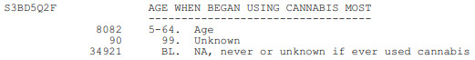
The moderating variable that I used for the statistical interaction is:

FOLLOWING IS AN PYTHON PROGRAM

import pandas import numpy import seaborn import scipy import matplotlib.pyplot as plt

nesarc = pandas.read_csv ('nesarc_pds.csv', low_memory=False)

Set PANDAS to show all columns in DataFrame

pandas.set_option('display.max_columns' , None)

Set PANDAS to show all rows in DataFrame

pandas.set_option('display.max_rows' , None)

nesarc.columns = map(str.upper , nesarc.columns)

pandas.set_option('display.float_format' , lambda x:'%f'%x)

Change my variables to numeric

nesarc['AGE'] = nesarc['AGE'].convert_objects(convert_numeric=True) nesarc['MAJORDEP12'] = nesarc['MAJORDEP12'].convert_objects(convert_numeric=True) nesarc['S1Q231'] = nesarc['S1Q231'].convert_objects(convert_numeric=True) nesarc['S3BQ1A5'] = nesarc['S3BQ1A5'].convert_objects(convert_numeric=True) nesarc['S3BD5Q2E'] = nesarc['S3BD5Q2E'].convert_objects(convert_numeric=True)

Subset my sample

subset1 = nesarc[(nesarc['AGE']>=18) & (nesarc['AGE']<=30) & nesarc['S3BQ1A5']==1] # Ages 18-30, cannabis users subsetc1 = subset1.copy()

Setting missing data

subsetc1['S1Q231']=subsetc1['S1Q231'].replace(9, numpy.nan) subsetc1['S3BQ1A5']=subsetc1['S3BQ1A5'].replace(9, numpy.nan) subsetc1['S3BD5Q2E']=subsetc1['S3BD5Q2E'].replace(99, numpy.nan) subsetc1['S3BD5Q2E']=subsetc1['S3BD5Q2E'].replace('BL', numpy.nan)

recode1 = {1: 9, 2: 8, 3: 7, 4: 6, 5: 5, 6: 4, 7: 3, 8: 2, 9: 1} # Frequency of cannabis use variable reverse-recode subsetc1['CUFREQ'] = subsetc1['S3BD5Q2E'].map(recode1) # Change the variable name from S3BD5Q2E to CUFREQ

subsetc1['CUFREQ'] = subsetc1['CUFREQ'].astype('category')

Raname graph labels for better interpetation

subsetc1['CUFREQ'] = subsetc1['CUFREQ'].cat.rename_categories(["2 times/year","3-6 times/year","7-11 times/year","Once a month","2-3 times/month","1-2 times/week","3-4 times/week","Nearly every day","Every day"])

Contingency table of observed counts of major depression diagnosis (response variable) within frequency of cannabis use groups (explanatory variable), in ages 18-30

contab1 = pandas.crosstab(subsetc1['MAJORDEP12'], subsetc1['CUFREQ']) print (contab1)

Column percentages

colsum=contab1.sum(axis=0) colpcontab=contab1/colsum print(colpcontab)

Chi-square calculations for major depression within frequency of cannabis use groups

print ('Chi-square value, p value, expected counts, for major depression within cannabis use status') chsq1= scipy.stats.chi2_contingency(contab1) print (chsq1)

Bivariate bar graph for major depression percentages with each cannabis smoking frequency group

plt.figure(figsize=(12,4)) # Change plot size ax1 = seaborn.factorplot(x="CUFREQ", y="MAJORDEP12", data=subsetc1, kind="bar", ci=None) ax1.set_xticklabels(rotation=40, ha="right") # X-axis labels rotation plt.xlabel('Frequency of cannabis use') plt.ylabel('Proportion of Major Depression') plt.show()

recode2 = {1: 10, 2: 9, 3: 8, 4: 7, 5: 6, 6: 5, 7: 4, 8: 3, 9: 2, 10: 1} # Frequency of cannabis use variable reverse-recode subsetc1['CUFREQ2'] = subsetc1['S3BD5Q2E'].map(recode2) # Change the variable name from S3BD5Q2E to CUFREQ2

sub1=subsetc1[(subsetc1['S1Q231']== 1)] sub2=subsetc1[(subsetc1['S1Q231']== 2)]

print ('Association between cannabis use status and major depression for those who lost a family member or a close friend in the last 12 months') contab2=pandas.crosstab(sub1['MAJORDEP12'], sub1['CUFREQ2']) print (contab2)

Column percentages

colsum2=contab2.sum(axis=0) colpcontab2=contab2/colsum2 print(colpcontab2)

Chi-square

print ('Chi-square value, p value, expected counts') chsq2= scipy.stats.chi2_contingency(contab2) print (chsq2)

Line graph for major depression percentages within each frequency group, for those who lost a family member or a close friend

plt.figure(figsize=(12,4)) # Change plot size ax2 = seaborn.factorplot(x="CUFREQ", y="MAJORDEP12", data=sub1, kind="point", ci=None) ax2.set_xticklabels(rotation=40, ha="right") # X-axis labels rotation plt.xlabel('Frequency of cannabis use') plt.ylabel('Proportion of Major Depression') plt.title('Association between cannabis use status and major depression for those who lost a family member or a close friend in the last 12 months') plt.show()

#

print ('Association between cannabis use status and major depression for those who did NOT lose a family member or a close friend in the last 12 months') contab3=pandas.crosstab(sub2['MAJORDEP12'], sub2['CUFREQ2']) print (contab3)

Column percentages

colsum3=contab3.sum(axis=0) colpcontab3=contab3/colsum3 print(colpcontab3)

Chi-square

print ('Chi-square value, p value, expected counts') chsq3= scipy.stats.chi2_contingency(contab3) print (chsq3)

Line graph for major depression percentages within each frequency group, for those who did NOT lose a family member or a close friend

plt.figure(figsize=(12,4)) # Change plot size ax3 = seaborn.factorplot(x="CUFREQ", y="MAJORDEP12", data=sub2, kind="point", ci=None) ax3.set_xticklabels(rotation=40, ha="right") # X-axis labels rotation plt.xlabel('Frequency of cannabis use') plt.ylabel('Proportion of Major Depression') plt.title('Association between cannabis use status and major depression for those who did NOT lose a family member or a close friend in the last 12 months') plt.show()

OUTPUT:

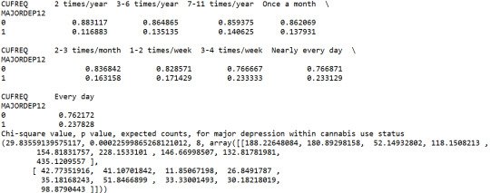
A Chi Square test of independence revealed that among cannabis users aged between 18 and 30 years old (subsetc1), the frequency of cannabis use (explanatory variable collapsed into 9 ordered categories) and past year depression diagnosis (response binary categorical variable) were significantly associated, X2 =29.83, 8 df, p=0.00022.

In the bivariate graph (C->C) presented above, we can see the correlation between frequency of cannabis use (explanatory variable) and major depression diagnosis in the past year (response variable). Obviously, we have a left-skewed distribution, which indicates that the more an individual (18-30) smoked cannabis, the better were the chances to have experienced depression in the last 12 months.

In the first place, for the moderating variable equal to 1, which is those whose a family member or a close friend died in the last 12 months (sub1), a Chi Square test of independence revealed that among cannabis users aged between 18 and 30 years old, the frequency of cannabis use (explanatory variable) and past year depression diagnosis (response variable) were not significantly associated, X2 =4.61, 9 df, p=0.86. As a result, since the chi-square value is quite small and the p-value is significantly large, we can assume that there is no statistical relationship between these two variables, when taking into account the subgroup of individuals who lost a family member or a close friend in the last 12 months.

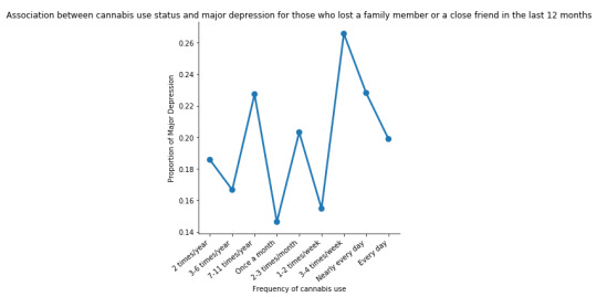
In the bivariate line graph (C->C) presented above, we can see the correlation between frequency of cannabis use (explanatory variable) and major depression diagnosis in the past year (response variable), in the subgroup of individuals whose a family member or a close friend died in the last 12 months (sub1). In fact, the direction of the distribution (fluctuation) does not indicate a positive relationship between these two variables, for those who experienced a family/close death in the past year.

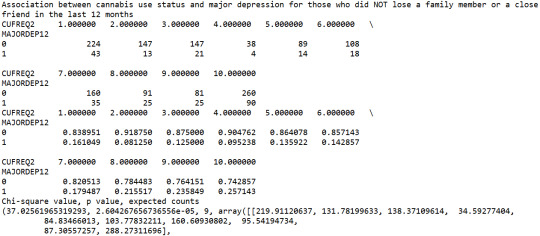
Subsequently, for the moderating variable equal to 2, which is those whose a family member or a close friend did not die in the last 12 months (sub2), a Chi Square test of independence revealed that among cannabis users aged between 18 and 30 years old, the frequency of cannabis use (explanatory variable) and past year depression diagnosis (response variable) were significantly associated, X2 =37.02, 9 df, p=2.6e-05 (p-value is written in scientific notation). As a result, since the chi-square value is quite large and the p-value is significantly small, we can assume that there is a positive relationship between these two variables, when taking into account the subgroup of individuals who did not lose a family member or a close friend in the last 12 months.

In the bivariate line graph (C->C) presented above, we can see the correlation between frequency of cannabis use (explanatory variable) and major depression diagnosis in the past year (response variable), in the subgroup of individuals whose a family member or a close friend did not die in the last 12 months (sub2). Obviously, the direction of the distribution indicates a positive relationship between these two variables, which means that the frequency of cannabis use directly affects the proportions of major depression, regarding the individuals who did not experience a family/close death in the last 12 months.

Summary

It seems that both the direction and the size of the relationship between frequency of cannabis use and major depression diagnosis in the last 12 months, is heavily affected by a death of a family member or a close friend in the same period. In other words, when the incident of a family/close death is present, the correlation is considerably weak, whereas when it is absent, the correlation is significantly strong and positive. Thus, the third variable moderates the association between cannabis use frequency and major depression diagnosis.

[usesofcannabis]

Generating a Correlation Coefficient

This assignment aims to statistically assess the evidence, provided by NESARC codebook, in favor of or against the association between cannabis use and mental illnesses, such as major depression and general anxiety, in U.S. adults. More specifically, since my research question includes only categorical variables, I selected three new quantitative variables from the NESARC codebook. Therefore, I redefined my hypothesis and examined the correlation between the age when the individuals began using cannabis the most (quantitative explanatory, variable “S3BD5Q2F”) and the age when they experienced the first episode of major depression and general anxiety (quantitative response, variables “S4AQ6A” and ”S9Q6A”). As a result, in the first place, in order to visualize the association between cannabis use and both depression and anxiety episodes, I used seaborn library to produce a scatterplot for each disorder separately and interpreted the overall patterns, by describing the direction, as well as the form and the strength of the relationships. In addition, I ran Pearson correlation test (Q->Q) twice (once for each disorder) and measured the strength of the relationships between each pair of quantitative variables, by numerically generating both the correlation coefficients r and the associated p-values. For the code and the output I used Spyder (IDE).

The three quantitative variables that I used for my Pearson correlation tests are:

  

FOLLWING IS A PYTHON PROGRAM TO CALCULATE CORRELATION

import pandas import numpy import seaborn import scipy import matplotlib.pyplot as plt

nesarc = pandas.read_csv ('nesarc_pds.csv' , low_memory=False)

Set PANDAS to show all columns in DataFrame

pandas.set_option('display.max_columns', None)

Set PANDAS to show all rows in DataFrame

pandas.set_option('display.max_rows', None)

nesarc.columns = map(str.upper , nesarc.columns)

pandas.set_option('display.float_format' , lambda x:'%f'%x)

Change my variables to numeric

nesarc['AGE'] = pandas.to_numeric(nesarc['AGE'], errors='coerce') nesarc['S3BQ4'] = pandas.to_numeric(nesarc['S3BQ4'], errors='coerce') nesarc['S4AQ6A'] = pandas.to_numeric(nesarc['S4AQ6A'], errors='coerce') nesarc['S3BD5Q2F'] = pandas.to_numeric(nesarc['S3BD5Q2F'], errors='coerce') nesarc['S9Q6A'] = pandas.to_numeric(nesarc['S9Q6A'], errors='coerce') nesarc['S4AQ7'] = pandas.to_numeric(nesarc['S4AQ7'], errors='coerce') nesarc['S3BQ1A5'] = pandas.to_numeric(nesarc['S3BQ1A5'], errors='coerce')

Subset my sample

subset1 = nesarc[(nesarc['S3BQ1A5']==1)] # Cannabis users subsetc1 = subset1.copy()

Setting missing data

subsetc1['S3BQ1A5']=subsetc1['S3BQ1A5'].replace(9, numpy.nan) subsetc1['S3BD5Q2F']=subsetc1['S3BD5Q2F'].replace('BL', numpy.nan) subsetc1['S3BD5Q2F']=subsetc1['S3BD5Q2F'].replace(99, numpy.nan) subsetc1['S4AQ6A']=subsetc1['S4AQ6A'].replace('BL', numpy.nan) subsetc1['S4AQ6A']=subsetc1['S4AQ6A'].replace(99, numpy.nan) subsetc1['S9Q6A']=subsetc1['S9Q6A'].replace('BL', numpy.nan) subsetc1['S9Q6A']=subsetc1['S9Q6A'].replace(99, numpy.nan)

Scatterplot for the age when began using cannabis the most and the age of first episode of major depression

plt.figure(figsize=(12,4)) # Change plot size scat1 = seaborn.regplot(x="S3BD5Q2F", y="S4AQ6A", fit_reg=True, data=subset1) plt.xlabel('Age when began using cannabis the most') plt.ylabel('Age when expirenced the first episode of major depression') plt.title('Scatterplot for the age when began using cannabis the most and the age of first the episode of major depression') plt.show()

data_clean=subset1.dropna()

Pearson correlation coefficient for the age when began using cannabis the most and the age of first the episode of major depression

print ('Association between the age when began using cannabis the most and the age of the first episode of major depression') print (scipy.stats.pearsonr(data_clean['S3BD5Q2F'], data_clean['S4AQ6A']))

Scatterplot for the age when began using cannabis the most and the age of the first episode of general anxiety

plt.figure(figsize=(12,4)) # Change plot size scat2 = seaborn.regplot(x="S3BD5Q2F", y="S9Q6A", fit_reg=True, data=subset1) plt.xlabel('Age when began using cannabis the most') plt.ylabel('Age when expirenced the first episode of general anxiety') plt.title('Scatterplot for the age when began using cannabis the most and the age of the first episode of general anxiety') plt.show()

Pearson correlation coefficient for the age when began using cannabis the most and the age of the first episode of general anxiety

print ('Association between the age when began using cannabis the most and the age of first the episode of general anxiety') print (scipy.stats.pearsonr(data_clean['S3BD5Q2F'], data_clean['S9Q6A']))

OUTPUT:

The scatterplot presented above, illustrates the correlation between the age when individuals began using cannabis the most (quantitative explanatory variable) and the age when they experienced the first episode of depression (quantitative response variable). The direction of the relationship is positive (increasing), which means that an increase in the age of cannabis use is associated with an increase in the age of the first depression episode. In addition, since the points are scattered about a line, the relationship is linear. Regarding the strength of the relationship, from the pearson correlation test we can see that the correlation coefficient is equal to 0.23, which indicates a weak linear relationship between the two quantitative variables. The associated p-value is equal to 2.27e-09 (p-value is written in scientific notation) and the fact that its is very small means that the relationship is statistically significant. As a result, the association between the age when began using cannabis the most and the age of the first depression episode is moderately weak, but it is highly unlikely that a relationship of this magnitude would be due to chance alone. Finally, by squaring the r, we can find the fraction of the variability of one variable that can be predicted by the other, which is fairly low at 0.05.

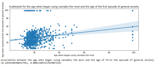
For the association between the age when individuals began using cannabis the most (quantitative explanatory variable) and the age when they experienced the first episode of anxiety (quantitative response variable), the scatterplot psented above shows a positive linear relationship. Regarding the strength of the relationship, the pearson correlation test indicates that the correlation coefficient is equal to 0.14, which is interpreted to a fairly weak linear relationship between the two quantitative variables. The associated p-value is equal to 0.0001, which means that the relationship is statistically significant. Therefore, the association between the age when began using cannabis the most and the age of the first anxiety episode is weak, but it is highly unlikely that a relationship of this magnitude would be due to chance alone. Finally, by squaring the r, we can find the fraction of the variability of one variable that can be predicted by the other, which is very low at 0.01.

[usesofcannabis]

Hypothesis Testing and Chi Square Test of Independence

This assignment aims to directly test my hypothesis by evaluating, based on a sample of 2412 U.S. cannabis users aged between 18 and 30 years old (subsetc2), my research question with the goal of generalizing the results to the larger population of NESARC survey, from where the sample has been drawn. Therefore, I statistically assessed the evidence, provided by NESARC codebook, in favor of or against the association between cannabis use and mental illnesses, such as major depression and general anxiety, in U.S. adults. As a result, in the first place I used crosstab function, in order to produce a contingency table of observed counts and percentages for each disorder separately. Next, I wanted to examine if the cannabis use status (1=Yes or 2=No) variable ‘S3BQ1A5’, which is a 2-level categorical explanatory variable, is correlated with depression (‘MAJORDEP12’) and anxiety (‘GENAXDX12’) disorders, which are both categorical response variables. Thus, I ran Chi-square Test of Independence (C->C) twice and calculated the χ-squared values and the associated p-values for each disorder, so that null and alternate hypothesis are specified. In addition, in order visualize the association between frequency of cannabis use and depression diagnosis, I used factorplot function to produce a bivariate graph. Furthermore, I used crosstab function once again and tested the association between the frequency of cannabis use (‘S3BD5Q2E’), which is a 10-level categorical explanatory variable, and major depression diagnosis, which is a categorical response variable. In this case, for my third Chi-square Test of Independence (C->C), after measuring the χ-square value and the p-value, in order to determine which frequency groups are different from the others, I performed a post hoc test, using Bonferroni Adjustment approach, since my explanatory variable has more than 2 levels. In the case of ten groups, I actually need to conduct 45 pair wise comparisons, but in fact I examined indicatively two and compared their p-values with the Bonferroni adjusted p-value, which is calculated by dividing p=0.05 by 45. By this way it is possible to identify the situations where null hypothesis can be safely rejected without making an excessive type 1 error. For the code and the output I used Spyder (IDE).

FOLLOWING IS A CODE WHICH IS USE TO CONDUCT

Chi Square Test

import pandas import numpy import scipy.stats import seaborn import matplotlib.pyplot as plt

nesarc = pandas.read_csv ('nesarc_pds.csv' , low_memory=False)

Set PANDAS to show all columns in DataFrame

pandas.set_option('display.max_columns', None)

Set PANDAS to show all rows in DataFrame

pandas.set_option('display.max_rows', None)

nesarc.columns = map(str.upper , nesarc.columns)

pandas.set_option('display.float_format' , lambda x:'%f'%x)

Change my variables to numeric

nesarc['AGE'] = pandas.to_numeric(nesarc['AGE'], errors='coerce') nesarc['S3BQ4'] = pandas.to_numeric(nesarc['S3BQ4'], errors='coerce') nesarc['S3BQ1A5'] = pandas.to_numeric(nesarc['S3BQ1A5'], errors='coerce') nesarc['S3BD5Q2B'] = pandas.to_numeric(nesarc['S3BD5Q2B'], errors='coerce') nesarc['S3BD5Q2E'] = pandas.to_numeric(nesarc['S3BD5Q2E'], errors='coerce') nesarc['MAJORDEP12'] = pandas.to_numeric(nesarc['MAJORDEP12'], errors='coerce') nesarc['GENAXDX12'] = pandas.to_numeric(nesarc['GENAXDX12'], errors='coerce')

Subset my sample

subset1 = nesarc[(nesarc['AGE']>=18) & (nesarc['AGE']<=30)] # Ages 18-30 subsetc1 = subset1.copy()

subset2 = nesarc[(nesarc['AGE']>=18) & (nesarc['AGE']<=30) & (nesarc['S3BQ1A5']==1)] # Cannabis users, ages 18-30 subsetc2 = subset2.copy()

Setting missing data for frequency and cannabis use, variables S3BD5Q2E, S3BQ1A5

subsetc1['S3BQ1A5']=subsetc1['S3BQ1A5'].replace(9, numpy.nan) subsetc2['S3BD5Q2E']=subsetc2['S3BD5Q2E'].replace('BL', numpy.nan) subsetc2['S3BD5Q2E']=subsetc2['S3BD5Q2E'].replace(99, numpy.nan)

Contingency table of observed counts of major depression diagnosis (response variable) within cannabis use (explanatory variable), in ages 18-30

contab1=pandas.crosstab(subsetc1['MAJORDEP12'], subsetc1['S3BQ1A5']) print (contab1)

Column percentages

colsum=contab1.sum(axis=0) colpcontab=contab1/colsum print(colpcontab)

Chi-square calculations for major depression within cannabis use status

print ('Chi-square value, p value, expected counts, for major depression within cannabis use status') chsq1= scipy.stats.chi2_contingency(contab1) print (chsq1)

Contingency table of observed counts of geberal anxiety diagnosis (response variable) within cannabis use (explanatory variable), in ages 18-30

contab2=pandas.crosstab(subsetc1['GENAXDX12'], subsetc1['S3BQ1A5']) print (contab2)

Column percentages

colsum2=contab2.sum(axis=0) colpcontab2=contab2/colsum2 print(colpcontab2)

Chi-square calculations for general anxiety within cannabis use status

print ('Chi-square value, p value, expected counts, for general anxiety within cannabis use status') chsq2= scipy.stats.chi2_contingency(contab2) print (chsq2)

#

Contingency table of observed counts of major depression diagnosis (response variable) within frequency of cannabis use (10 level explanatory variable), in ages 18-30

contab3=pandas.crosstab(subset2['MAJORDEP12'], subset2['S3BD5Q2E']) print (contab3)

Column percentages

colsum3=contab3.sum(axis=0) colpcontab3=contab3/colsum3 print(colpcontab3)

Chi-square calculations for mahor depression within frequency of cannabis use groups

print ('Chi-square value, p value, expected counts for major depression associated frequency of cannabis use') chsq3= scipy.stats.chi2_contingency(contab3) print (chsq3)

recode1 = {1: 9, 2: 8, 3: 7, 4: 6, 5: 5, 6: 4, 7: 3, 8: 2, 9: 1} # Dictionary with details of frequency variable reverse-recode subsetc2['CUFREQ'] = subsetc2['S3BD5Q2E'].map(recode1) # Change variable name from S3BD5Q2E to CUFREQ

subsetc2["CUFREQ"] = subsetc2["CUFREQ"].astype('category')

Rename graph labels for better interpretation

subsetc2['CUFREQ'] = subsetc2['CUFREQ'].cat.rename_categories(["2 times/year","3-6 times/year","7-11 times/years","Once a month","2-3 times/month","1-2 times/week","3-4 times/week","Nearly every day","Every day"])

Graph percentages of major depression within each cannabis smoking frequency group

plt.figure(figsize=(12,4)) # Change plot size ax1 = seaborn.factorplot(x="CUFREQ", y="MAJORDEP12", data=subsetc2, kind="bar", ci=None) ax1.set_xticklabels(rotation=40, ha="right") # X-axis labels rotation plt.xlabel('Frequency of cannabis use') plt.ylabel('Proportion of Major Depression') plt.show()

Post hoc test, pair comparison of frequency groups 1 and 9, 'Every day' and '2 times a year'

recode2 = {1: 1, 9: 9} subsetc2['COMP1v9']= subsetc2['S3BD5Q2E'].map(recode2)

Contingency table of observed counts

ct4=pandas.crosstab(subsetc2['MAJORDEP12'], subsetc2['COMP1v9']) print (ct4)

Column percentages

colsum4=ct4.sum(axis=0) colpcontab4=ct4/colsum4 print(colpcontab4)

Chi-square calculations for pair comparison of frequency groups 1 and 9, 'Every day' and '2 times a year'

print ('Chi-square value, p value, expected counts, for pair comparison of frequency groups -Every day- and -2 times a year-') cs4= scipy.stats.chi2_contingency(ct4) print (cs4)

Post hoc test, pair comparison of frequency groups 2 and 6, 'Nearly every day' and 'Once a month'

recode3 = {2: 2, 6: 6} subsetc2['COMP2v6']= subsetc2['S3BD5Q2E'].map(recode3)

Contingency table of observed counts

ct5=pandas.crosstab(subsetc2['MAJORDEP12'], subsetc2['COMP2v6']) print (ct5)

Column percentages

colsum5=ct5.sum(axis=0) colpcontab5=ct5/colsum5 print(colpcontab5)

Chi-square calculations for pair comparison of frequency groups 2 and 6, 'Nearly every day' and 'Once a month'

print ('Chi-square value, p value, expected counts for pair comparison of frequency groups -Nearly every day- and -Once a month-') cs5= scipy.stats.chi2_contingency(ct5) print (cs5)

OUTPUT:

When examining the patterns of association between major depression (categorical response variable) and cannabis use status (categorical explanatory variable), a chi-square test of independence revealed that among young adults aged between 18 and 30 years old (subsetc1), those who were cannabis users, were more likely to have been diagnosed with major depression in the last 12 months (18%), compared to the non-users (8.4%), X2 =171.6, 1 df, p=3.16e-39 (p-value is written in scientific notation). As a result, since our p-value is extremely small, the data provides significant evidence against the null hypothesis. Thus, we reject the null hypothesis and accept the alternate hypothesis, which indicates that there is a positive correlation between cannabis use and depression diagnosis.

When testing the correlation between general anxiety (categorical response variable) and cannabis use status (categorical explanatory variable), a chi-square test of independence revealed that among young adults aged between 18 and 30 years old (subsetc1), those who were cannabis users, were more likely to have been diagnosed with general anxiety in the last 12 months (3.8%), compared to the non-users (1.6%), X2 =40.22, 1 df, p=2.26e-10 (p-value is written in scientific notation). As a result, since our p-value is again extremely small, the data provides significant evidence against the null hypothesis. Thus, we reject the null hypothesis and accept the alternate hypothesis, which indicates that there is a positive correlation between cannabis use and anxiety diagnosis.

A Chi Square test of independence revealed that among cannabis users aged between 18 and 30 years old (subsetc2), the frequency of cannabis use (explanatory variable collapsed into 10 ordered categories) and past year depression diagnosis (response binary categorical variable) were significantly associated, X2 =35.18, 10 df, p=0.00011.

In the bivariate graph (C->C) presented above, we can see the correlation between frequency of cannabis use (explanatory variable) and major depression diagnosis in the past year (response variable). Obviously, we have a left-skewed distribution, which indicates that the more an individual (18-30) smoked cannabis, the better were the chances to have experienced depression in the last 12 months.

The post hoc comparison (Bonferroni Adjustment) of rates of major depression by the pair of “Every day” and “2 times a year” frequency categories, revealed that the p-value is 0.00019 and the percentages of major depression diagnosis for each frequency group are 23.7% and 11.6% respectively. As a result, since the p-value is smaller than the Bonferroni adjusted p-value (adj p-value = 0.05 / 45 = 0.0011>0.00019), we can assume that these two rates are significantly different from one another. Therefore, we reject the null hypothesis and accept the alternate.

Similarly, the post hoc comparison (Bonferroni Adjustment) of rates of major depression by the pair of "Nearly every day” and “once a month” frequency categories, indicated that the p-value is 0.046 and the proportions of major depression diagnosis for each frequency group are 23.3% and 13.7% respectively. As a result, since the p-value is larger than the Bonferroni adjusted p-value (adj p-value = 0.05 / 45 = 0.0011<0.046), we can assume that these two rates are not significantly different from one another. Therefore, we accept the null hypothesis.

[usesofcannabis]

ANALYSIS OF VARIANCE OF EFFECTS BY CONSUMING CANNABIS

This assignment aims to directly test my hypothesis by evaluating, based on a sample of 2412 U.S. cannabis users aged between 18 and 30 years old (subsetc5), my research question with the goal of generalizing the results to the larger population of NESARC survey, from where the sample has been drawn. Therefore, I statistically assessed the evidence, provided by NESARC codebook, in favor of or against the association between cannabis use and mental illnesses, such as major depression and general anxiety, in U.S. adults. As a result, in the first place I used ols function in order to examine if depression (‘MAJORDEP12’) and anxiety ('GENAXDX12’) disorders, which are both categorical explanatory variables, are correlated with the quantity of joints smoked per day when using the most ('S3BQ4’), which is a quantitative response variable. Thus, I ran ANOVA (Analysis Of Variance) method (C->Q) twice and calculated the F-statistics and the associated p-values for each disorder separately, so that null and alternate hypothesis are specified. Furthermore, I used ols function once again and tested the association between the frequency of cannabis use ('S3BD5Q2E’), which is a 10-level categorical explanatory variable, and the quantity of joints smoked per day when using the most ('S3BQ4’), which is a quantitative response variable. In this case, for my third one-way ANOVA (C->Q), after measuring the F-statistic and the p-value, I used Tukey HSDT to perform a post hoc test, that conducts post hoc paired comparisons in the context of my ANOVA, since my explanatory variable has more than 2 levels. By this way it is possible to identify the situations where null hypothesis can be safely rejected without making an excessive type 1 error. In addition, both means and standard deviations of joints quantity response variable, were measured separately in each ANOVA, grouped by the explanatory variables (depression, anxiety and frequency of cannabis use) using the groupby function. For the code and the output I used Spyder (IDE).

When examining the association between the number of joints smoked per day (quantitative response variable) and the past 12 months major depression diagnosis (categorical explanatory variable), an Analysis of Variance (ANOVA) revealed that among cannabis users aged between 18 and 30 years old (subsetc5), those diagnosed with major depression reported smoking slightly more joints per day (Mean=3.04, s.d. ±5.22) compared to those without major depression (Mean=2.39, s.d. ±4.16), F(1, 2368)=7.682, p=0.00562<0.05. As a result, since our p-value is extremely small, the data provides significant evidence against the null hypothesis. Thus, we reject the null hypothesis and accept the alternate hypothesis, which indicates that there is a positive correlation between depression diagnosis and quantity of joints smoked per day.

When testing the association between the number of joints smoked per day (quantitative response variable) and the past 12 months general anxiety diagnosis (categorical explanatory variable), an Analysis of Variance (ANOVA) revealed that among cannabis users aged between 18 and 30 years old (subsetc5), those diagnosed with general anxiety reported smoking marginally equal quantity of joints per day (Mean=2.68, s.d. ±3.15) compared to those without general anxiety (Mean=2.5, s.d. ±4.42), F(1, 2368)=0.1411, p=0.707>0.05. As a result, since our p-value is significantly large, in this case the data is not considered to be surprising enough when the null hypothesis is true. Consequently, there are not enough evidence to reject the null hypothesis and accept the alternate, thus there is no positive association between anxiety diagnosis and quantity of joints smoked per day.

  

ANOVA revealed that among daily, cannabis users aged 18 to 30 years old (subsetc5), frequency of cannabis use (collapsed into 10 ordered categories, which is the categorical explanatory variable) and number of joints smoked per day (quantitative response variable) were relatively associated, F (9, 2349)=52.65, p=1.76e-87<0.05 (p value is written in scientific notation). Post hoc comparisons of mean number of joints smoked per day by pairs of cannabis use frequency categories, revealed that those individuals using cannabis every day (or nearly every day) reported smoking significantly more joints on average daily (every day: Mean=5.66, s.d. ±7.8, nearly every day: Mean=3.73, s.d. ±4.46) compared to those using 1 to 2 times per weak (Mean=1.85, s.d. ±1.81), or less. As a result, there are some pair cases in which using frequency and smoking quantity of cannabis, are positive correlated.

In order to conduct post hoc paired comparisons in the context of my ANOVA, examining the association between frequency of cannabis use and number of joints smoked per day when using the most, I used the Tukey HSD test. The table presented above, illustrates the differences in smoking quantity for each cannabis use frequency group and help us identify the comparisons in which we can reject the null hypothesis and accept the alternate, that is, in which reject equals true. In cases where reject equals false, rejecting the null hypothesis resulting in inflating a type 1 error.

FOLLOWING IS A PYTHON PROGRAM WHICH I HAVE USE ANAYLSIS THE VARIANCE

import pandas import numpy import statsmodels.formula.api as smf import statsmodels.stats.multicomp as multi nesarc = pandas.read_csv ('nesarc_pds.csv' , low_memory=False) # load NESARC dataset

Set PANDAS to show all columns in DataFrame

pandas.set_option('display.max_columns', None)

Set PANDAS to show all rows in DataFrame

pandas.set_option('display.max_rows', None)

nesarc.columns = map(str.upper , nesarc.columns)

pandas.set_option('display.float_format' , lambda x:'%f'%x)

Change my variables to numeric

nesarc['AGE'] = nesarc['AGE'].convert_objects(convert_numeric=True) nesarc['S3BQ4'] = nesarc['S3BQ4'].convert_objects(convert_numeric=True) nesarc['S3BQ1A5'] = nesarc['S3BQ1A5'].convert_objects(convert_numeric=True) nesarc['S3BD5Q2B'] = nesarc['S3BD5Q2B'].convert_objects(convert_numeric=True) nesarc['S3BD5Q2E'] = nesarc['S3BD5Q2E'].convert_objects(convert_numeric=True) nesarc['MAJORDEP12'] = nesarc['MAJORDEP12'].convert_objects(convert_numeric=True) nesarc['GENAXDX12'] = nesarc['GENAXDX12'].convert_objects(convert_numeric=True)

Subset my sample

subset5 = nesarc[(nesarc['AGE']>=18) & (nesarc['AGE']<=30) & (nesarc['S3BQ1A5']==1)] # Cannabis users, ages 18-30 subsetc5 = subset5.copy()

Setting missing data for quantity of cannabis (measured in joints), variable S3BQ4

subsetc5['S3BQ4']=subsetc5['S3BQ4'].replace(99, numpy.nan) subsetc5['S3BQ4']=subsetc5['S3BQ4'].replace('BL', numpy.nan)

sub1 = subsetc5[['S3BQ4', 'MAJORDEP12']].dropna()

Using ols function for calculating the F-statistic and the associated p value

Depression (categorical, explanatory variable) and joints quantity (quantitative, response variable) correlation

model1 = smf.ols(formula='S3BQ4 ~ C(MAJORDEP12)', data=sub1) results1 = model1.fit() print (results1.summary())

Measure mean and spread for categorical variable MAJORDEP12, major depression

print ('Means for joints quantity by major depression status') m1= sub1.groupby('MAJORDEP12').mean() print (m1)

print ('Standard deviations for joints quantity by major depression status') sd1 = sub1.groupby('MAJORDEP12').std() print (sd1)

sub2 = subsetc5[['S3BQ4', 'GENAXDX12']].dropna()

Using ols function for calculating the F-statistic and the associated p value

Anxiety (categorical, explanatory variable) and joints quantity (quantitative, response variable) correlation

model2 = smf.ols(formula='S3BQ4 ~ C(GENAXDX12)', data=sub2) results2 = model2.fit() print (results2.summary())

Measure mean and spread for categorical variable GENAXDX12, general anxiety

print ('Means for joints quantity by major general anxiety status') m2= sub2.groupby('GENAXDX12').mean() print (m2)

print ('Standard deviations for joints quantity by general anxiety status') sd2 = sub2.groupby('GENAXDX12').std() print (sd2)

#

Setting missing data for frequency of cannabis use, variable S3BD5Q2E

subsetc5['S3BD5Q2E']=subsetc5['S3BD5Q2E'].replace(99, numpy.nan) subsetc5['S3BD5Q2E']=subsetc5['S3BD5Q2E'].replace('BL', numpy.nan)

sub3 = subsetc5[['S3BQ4', 'S3BD5Q2E']].dropna()

Using ols function for calculating the F-statistic and associated p value

Frequency of cannabis use (10 level categorical, explanatory variable) and joints quantity (quantitative, response variable) correlation

model3 = smf.ols(formula='S3BQ4 ~ C(S3BD5Q2E)', data=sub3).fit() print (model3.summary())

Measure mean and spread for categorical variable S3BD5Q2E, frequency of cannabis use

print ('Means for joints quantity by frequency of cannabis use status') mc2= sub3.groupby('S3BD5Q2E').mean() print (mc2)

print ('Standard deviations for joints quantity by frequency of cannabis use status') sdc2 = sub3.groupby('S3BD5Q2E').std() print (sdc2)

Run a post hoc test (paired comparisons), using Tukey HSDT

mc1 = multi.MultiComparison(sub3['S3BQ4'], sub3['S3BD5Q2E']) res1 = mc1.tukeyhsd() print(res1.summary())