atillathebunny - Tumblr blog

atillathebunny · 4 years ago

Text

logistic regression

This week I did my regression in both SAS and python. I felt SAS was much easier to get the odds ratio out of as in python I had to calculate it and the confidence interval for the odds ratio.

I have run 5 models in logistic regression in both SAS and python. To do this I created 5 binary variables.

The response variable democratic with polity score <=0 being 0 and polity score >0 being 1

The explanatory variabled employratebin, femaleemployratebin, maleemployratebin, and employgap bin with 0 being below the mean and 1 being >= to the means of employrate, femaleemplyrate, maleemployrate, and employgap

Their are 4 models with 1 explanatory variable each and 1 with 2 explanatory variables which will be discussed in the analysises below.

SAS

code

/* get access to course datasets*/

LIBNAME mydata "/courses/d1406ae5ba27fe300 " access=readonly;

/* pick specific data set*/

DATA new; set mydata.gapminder;

/* get the employee rates and democracy scores*/

LABEL femaleemployrate="% Females 15+ Employed 2007"

employrate="% Population 15+ Employed 2007"

polityscore="Polity Democracy Score 2009";

/* add a secondary variable of male employment rate % estimate*/

maleemployrate = employrate * 2 - femaleemployrate;

/* correction for 2 countries who do not have 50/50 split male to female*/

if country = "Qatar" then maleemployrate = ((4*employrate - femaleemployrate)/3);

if country = "United Arab Emirates" then maleemployrate = (3* employrate - femaleemployrate)/2;

/* Label the male employment rate */

LABEL maleemployrate=" Estimate of % Males 15+ Employed 2007" ;

/* create a secondary variable for gap in employment */

gaprate = maleemployrate - femaleemployrate;

/* Label the gap employment rate */

LABEL gaprate= "Gap between of % Males and Females 15+ Employed 2007" ;

/*create a binary response variable*/

if polityscore =. then polityscore = .;

else if polityscore <= 0 then democratic = 0;

else democratic = 1;

LABEL democratic ="Polity Democracy Score > 0 in 2009";

/*create binary explanatory variables*/

if employrate =. then employratebin = .;

else if employrate <= 58.649 then employratebin = 0;

else employratebin = 1;

if femaleemployrate =. then femaleemployratebin = .;

else if femaleemployrate <= 47.55 then femaleemployratebin = 0;

else femaleemployratebin = 1;

if maleemployrate =. then maleemployratebin = .;

else if femaleemployrate <= 69.48 then maleemployratebin = 0;

else maleemployratebin = 1;

if gaprate =. then gapratequant = .;

else if gaprate <= 21.93 then gapratebin = 0;

else gapratebin = 1;

PROC SORT; by country;

/*logistic models*/

Proc logistic descending; model democratic = employratebin;

Proc logistic descending; model democratic = femaleemployratebin;

Proc logistic descending; model democratic = maleemployratebin;

Proc logistic descending; model democratic = gapratebin;

Proc logistic descending; model democratic = gapratebin maleemployratebin;

RUN;

logistic models and analysis

First I ran 4 models with a binary value for employment rate, female employment rate, male employment rate, and employment gap being either below the mean or the mean or above against democratic (polity score <=0 or >0.

The models show that neither employratebin with a p of 0.2129 nor femaleemployratebin with a p of 0.9145 are statistically significant. So I do not go further with those models.

Both maleemployratebin and gapratebin with p of 0.0074 and p of 0.0324 are statistically significant. Both have odds ratios with a 95% confidence interval below 0. The odds ration of maleemployratebin is 0.387 (95% odds ratio between 0.193 and 0.775). The odds ration of gapratebin is 0.479 (95% odds ratio between 0.244 and 0.940).

This means that those countries with male employment at or above the mean are 0.387 times less likely to be democatic then those below the mean; a surprising finding.

Additionally, those countries with a gender pay gap are 0.479 times less likely to be democratic, which again was very unexpected.

My next model uses both the binary male employment rate and the binary gap rate

The results here show that gapratebin was a confounding variable and should be dropped.

This being said, I do not feel the male employment model is very useful as it strips away so much nuance. Previous analysis has shown that the relationship between employment and democracy is more u shaped.

Python

code

# -*- coding: utf-8 -*-

"""

Script to load in gapminder data and

male employment rates are estimated and gap in rate is computed

explores the relationship between democracy and employment

multiplelogistic regression analysis

"""

# load libraries

import pandas as pd

import numpy as np

import statsmodels.formula.api as smf

# load data

data = pd.read_csv(

'D:/Users/jesnr/Dropbox/coursera/data management and visualization/gapminder data.csv', low_memory=(False))

# toprevent runtime errors

#pd.set_option('display.float_format', lambda x: '%f'%x)

# change data to numeric

data['femaleemployrate'] = pd.to_numeric(

data['femaleemployrate'], errors='coerce')

data['employrate'] = pd.to_numeric(data['employrate'], errors='coerce')

data['polityscore'] = pd.to_numeric(data['polityscore'], errors='coerce')

# add in secondary variables

# estimate male employment rate

maleemployrate = []

for i, rate in enumerate(data['employrate']):

if data['country'][i] == "Qatar":

maleemployrate.append(((4*rate - data['femaleemployrate'][i])/3))

elif (data['country'][i] == "United Arab Emirates"):

maleemployrate.append((3 * rate - data['femaleemployrate'][i])/2)

else:

maleemployrate.append(rate * 2 - data['femaleemployrate'][i])

data['maleemployrate'] = maleemployrate

# determine employment gap:

employgap = []

for i, rate in enumerate(data['maleemployrate']):

employgap.append(rate - data['femaleemployrate'][i])

data['employgap'] = employgap

# make corrections for Qatar and UAE

data.loc[data['country'] == 'Qatar']['maleemployrate'] = (

4 * data.loc[data['country'] == 'Qatar']['employrate'] - 3 * data.loc[data['country'] == 'Qatar']['femaleemployrate'])

data.loc[data['country'] == 'United Arab Emirates']['maleemployrate'] = (

4 * data.loc[data['country'] == 'United Arab Emirates']['employrate'] - 3 * data.loc[data['country'] == 'United Arab Emirates']['femaleemployrate'])

# get rid of the nan's

data =data.dropna(subset = ['polityscore', 'employrate','femaleemployrate','maleemployrate','employgap' ])

# create the binary variables

def democracy(polity):

if polity <=0:

return 0

return 1

data['democratic'] = [democracy(polity) for polity in data['polityscore']]

def binvar(val, avg):

if val <=avg:

return 0

return 1

data['employratebin'] = [binvar(val,58.649) for val in data['employrate']]

data['femaleemployratebin'] = [binvar(val, 47.55) for val in data['femaleemployrate']]

data['maleemployratebin'] = [binvar(val, 69.48) for val in data['maleemployrate']]

data['gapratebin'] = [binvar(val, 21.93) for val in data['employgap']]

#logistic regression models

lr= smf.logit(formula = 'democratic~employratebin',data=data).fit()

print(lr.summary())

params = lr.params

conf = lr.conf_int()

conf['OR'] = params

conf.columns = ['Lower CI', 'Upper CI', 'Odds Ratio']

print(np.exp(conf))

print()

lr= smf.logit(formula = 'democratic~femaleemployratebin',data=data).fit()

print(lr.summary())

params = lr.params

conf = lr.conf_int()

conf['OR'] = params

conf.columns = ['Lower CI', 'Upper CI', 'Odds Ratio']

print(np.exp(conf))

print()

lr= smf.logit(formula = 'democratic~maleemployratebin',data=data).fit()

print(lr.summary())

params = lr.params

conf = lr.conf_int()

conf['OR'] = params

conf.columns = ['Lower CI', 'Upper CI', 'Odds Ratio']

print(np.exp(conf))

print()

lr= smf.logit(formula = 'democratic~gapratebin',data=data).fit()

print(lr.summary())

params = lr.params

conf = lr.conf_int()

conf['OR'] = params

conf.columns = ['Lower CI', 'Upper CI', 'Odds Ratio']

print(np.exp(conf))

print()

lr= smf.logit(formula = 'democratic~gapratebin + maleemployratebin',data=data).fit()

print(lr.summary())

params = lr.params

conf = lr.conf_int()

conf['OR'] = params

conf.columns = ['Lower CI', 'Upper CI', 'Odds Ratio']

print(np.exp(conf))

print()

logistic models and analysis

The models show that neither employratebin with a p of 0.2129 nor femaleemployratebin with a p of 0.9145 are statistically significant. So I do not go further with those models.

This means that those countries with male employment at or above the mean are 0.387times less likely to be democatic then those below the mean; a surprising finding.

Additionally, those countries with a gender pay gap are 0.479 times less likely to be democratic, which again was very unexpected.

My next model uses both the binary male employment rate and the binary gap rate

The results here show that gapratebin was a confounding variable and should be dropped.

#coursera #data science

0 notes

atillathebunny · 4 years ago

Text

Multiple Regression Model

This week I try to find a multiple regression model to predict the polity democracy score. I had limited success with this, but found that the best models did not use my calculated variables but did use the actual data in the Gapminder data set. As always I shall do my analysis twice, once in SAS and then again in python.

What took the longest this week was playing around with different models to find one which was both statistically significant and had reasonable residuals.

SAS

code

/* get access to course datasets*/

LIBNAME mydata "/courses/d1406ae5ba27fe300 " access=readonly;

/* pick specific data set*/

DATA new; set mydata.gapminder;

/* get the employee rates and democracy scores*/

LABEL femaleemployrate="% Females 15+ Employed 2007"

employrate="% Population 15+ Employed 2007"

polityscore="Polity Democracy Score 2009";

/* add a secondary variable of male employment rate % estimate*/

maleemployrate = employrate * 2 - femaleemployrate;

/* correction for 2 countries who do not have 50/50 split male to female*/

if country = "Qatar" then maleemployrate = ((4*employrate - femaleemployrate)/3);

if country = "United Arab Emirates" then maleemployrate = (3* employrate - femaleemployrate)/2;

/* Label the male employment rate */

LABEL maleemployrate=" Estimate of % Males 15+ Employed 2007" ;

/* create a secondary variable for gap in employment */

gaprate = maleemployrate - femaleemployrate;

/* Label the gap employment rate */

LABEL gaprate= "Gap between of % Males and Females 15+ Employed 2007" ;

/*centre means*/

PROC STANDARD MEAN=0 OUT=xdata;

VAR employrate femaleemployrate maleemployrate gaprate ;

PROC means data = xdata;

Var employrate femaleemployrate maleemployrate gaprate ;

/*model and plots*/

PROC GLM data = xdata PLOTS(unpack) = ALL ;

model polityscore = employrate femaleemployrate femaleemployrate*femaleemployrate / clparm ;

output residual = res student = stdres out = results;

PROC gplot ;

label stdres = "standard residual" country = "Country";

plot stdres*country/vref = 0;

/*partial plots*/

data partial;

set new;

femaleemployrate2 = femaleemployrate*femaleemployrate;

run;

PROC reg plots = partial;

model polityscore = employrate femaleemployrate femaleemployrate2/partial;

run;

Regression model, plots, and analysis

My final model is

polity score = 5.049 -0.377 *(employeerate - mean) + 0.254*(femaleemployrate-mean) - 0.006*(femaleemployrate-mean)^2

Please note that all of the parameters had p's of 0.0001 or below.

This means that when a country has a mean employment rate and mea female employment rate, the polity score is 5.049. For every 1% rise in population employment rate, there is a decrease in pooty score of 0.377. For every 1% rise in femaleemployment rate there is an increase in polity score of 0.254 and for every 1% rise in the square of femaleemployment rate there is a decrease of 0.006 in the polity score.

The r-square is .2314 which means 23.14% of the polity score is explained by the employment rate and female employment rate of a country.

The female employment rate is a confounder to the employment rate.

However when looking at the diagnostic plot, the residuals do indicate the model may have flaws.

The Q-Q plot does show a slight pattern to the residuals with extreme values being below the line and middling values being above the line, showing the distribution varies from a normal one.

Additionally, the residual plot shows a 1 value at -3 standard deviations and 6 values at -2.5 standard deviaions which is more than we would expect if this model was a good one.

This being said, none of the outliers are leveraged, Although there are many leveraged points, all of them are within 2 standard deviations which does give some support to the model.

Addditionally the partial plots all show a trend, which gives support to the model.

It is likely that adding on other variables which I have not been exploring would improve this model. But as it stands, it can be used to explain 23.14% of the polity democracy score.

Python

As I do each week, I will now repeat the analysis in python code

# -*- coding: utf-8 -*-

"""

Script to load in gapminder data and

male employment rates are estimated and gap in rate is computed

explores the relationship between democracy and employment

multiple regression analysis

"""

# load libraries

import pandas as pd

import statsmodels.formula.api as smf

from sklearn.preprocessing import scale

import statsmodels.api as sm

import matplotlib.pyplot as plt

import seaborn as sb

# load data

data = pd.read_csv(

'D:/Users/jesnr/Dropbox/coursera/data management and visualization/gapminder data.csv', low_memory=(False))

# toprevent runtime errors

#pd.set_option('display.float_format', lambda x: '%f'%x)

# change data to numeric

data['femaleemployrate'] = pd.to_numeric(

data['femaleemployrate'], errors='coerce')

data['employrate'] = pd.to_numeric(data['employrate'], errors='coerce')

data['polityscore'] = pd.to_numeric(data['polityscore'], errors='coerce')

# add in secondary variables

# estimate male employment rate

maleemployrate = []

for i, rate in enumerate(data['employrate']):

if data['country'][i] == "Qatar":

maleemployrate.append(((4*rate - data['femaleemployrate'][i])/3))

elif (data['country'][i] == "United Arab Emirates"):

maleemployrate.append((3 * rate - data['femaleemployrate'][i])/2)

else:

maleemployrate.append(rate * 2 - data['femaleemployrate'][i])

data['maleemployrate'] = maleemployrate

# determine employment gap:

employgap = []

for i, rate in enumerate(data['maleemployrate']):

employgap.append(rate - data['femaleemployrate'][i])

data['employgap'] = employgap

# make corrections for Qatar and UAE

data.loc[data['country'] == 'Qatar']['maleemployrate'] = (

4 * data.loc[data['country'] == 'Qatar']['employrate'] - 3 * data.loc[data['country'] == 'Qatar']['femaleemployrate'])

data.loc[data['country'] == 'United Arab Emirates']['maleemployrate'] = (

4 * data.loc[data['country'] == 'United Arab Emirates']['employrate'] - 3 * data.loc[data['country'] == 'United Arab Emirates']['femaleemployrate'])

# get rid of the nan's

data =data.dropna(subset = ['polityscore', 'employrate'])

# centre the explanatory variables

data['xemployrate'] = scale(data['employrate'],with_std=False)

data['xfemaleemployrate'] = scale(data['femaleemployrate'],with_std=False)

data['xmaleemployrate'] = scale(data['maleemployrate'],with_std=False)

data['xemploygap'] = scale(data['employgap'],with_std=False)

print("means")

print(data.mean())

print()

print("standard deviations")

print(data.std())

print()

# multiple regression model

print('OLS regression model for the association between employment and polity score')

model = smf.ols(formula='polityscore~xemployrate+xfemaleemployrate+I(xfemaleemployrate**2)',data=data).fit()

print(model.summary())

print()

#error examination in residual plots

#qqplot

plt.figure()

qq = sm.qqplot(model.resid, line = 'r')

# plot of residuals

plt.figure()

stdres = pd.DataFrame(model.resid_pearson)

residplot = plt.plot(stdres, 'o', ls = 'None')

l = plt.axhline(y=0,color = 'r')

#regression diagnostic plot

plt.figure()

regdiagplot1 = plt.figure(figsize=(12,8))

regdiagplot1 = sm.graphics.plot_regress_exog(model,"xemployrate", fig = regdiagplot1)

plt.figure()

regdiagplot2 = plt.figure(figsize=(12,8))

regdiagplot2 = sm.graphics.plot_regress_exog(model,"xfemaleemployrate", fig = regdiagplot2)

plt.figure()

#leverage plot

plt.figure()

levplot = sm.graphics.influence_plot(model, size = 8)

Regression model, plots, and analysis

My final model is

polity score = 4.899 -0.377 *(employeerate - mean) + 0.248*(femaleemployrate-mean) - 0.006*(femaleemployrate-mean)^2

Please note that all of the parameters had p's of 0.0001 or below.

This means that when a country has a mean employment rate and mea female employment rate, the polity score is 4.899. For every 1% rise in population employment rate, there is a decrease in pooty score of 0.377. For every 1% rise in femaleemployment rate there is an increase in polity score of 0.248 and for every 1% rise in the square of femaleemployment rate there is a decrease of 0.006 in the polity score.

The r-square is .231 which means 23.1% of the polity score is explained by the employment rate and female employment rate of a country.

The female employment rate is a confounder to the employment rate.

However when looking at the diagnostic plot, the residuals do indicate the model may have flaws.

The Q-Q plot does show a slight pattern to the residuals with extreme values being below the line and middling values being above the line, showing the distribution varies from a normal one.

Additionally, the residual plot shows a 1 value at -3 standard deviations and 6 values at -2.5 standard deviaions which is more than we would expect if this model was a good one.

This being said, none of the outliers are leveraged, Although there are many leveraged points, all of them are within 2 standard deviations which does give some support to the model.

Addditionally the partial plots all show a trend, which gives support to the model. The female employment rate does show a curve, which gives evidence as to why the (female employment rate)^2 should be in the model.

It is likely that adding on other variables which I have not been exploring would improve this model. But as it stands, it can be used to explain 23.1% of the polity democracy score.

#coursera #data science

0 notes

atillathebunny · 4 years ago

Text

a Basic Linear Regression Model

As always I will repeat this analysis in both python and SAS. I found both equally easy to use this week, although SAS took less commands to get out more information. In both SAS and python, there were special commands that could be use to center the mean. A little bit of internet research was all that was needed.

I will be making 4 regression models

1. polity score by employment rate

2. polity score by female employment rate

3. polty score by male employment rate

4. polity score by gender gap in employment rate

SAS

code

/* get access to course datasets*/

LIBNAME mydata "/courses/d1406ae5ba27fe300 " access=readonly;

/* pick specific data set*/

DATA new; set mydata.gapminder;

/* get the employee rates and democracy scores*/

LABEL femaleemployrate="% Females 15+ Employed 2007"

employrate="% Population 15+ Employed 2007"

polityscore="Polity Democracy Score 2009";

/* add a secondary variable of male employment rate % estimate*/

maleemployrate = employrate * 2 - femaleemployrate;

/* correction for 2 countries who do not have 50/50 split male to female*/

if country = "Qatar" then maleemployrate = ((4*employrate - femaleemployrate)/3);

if country = "United Arab Emirates" then maleemployrate = (3* employrate - femaleemployrate)/2;

/* Label the male employment rate */

LABEL maleemployrate=" Estimate of % Males 15+ Employed 2007" ;

/* create a secondary variable for gap in employment */

gaprate = maleemployrate - femaleemployrate;

/* Label the gap employment rate */

LABEL gaprate= "Gap between of % Males and Females 15+ Employed 2007" ;

/*centre means*/

PROC STANDARD MEAN=0 OUT=xdata;

VAR employrate femaleemployrate maleemployrate gaprate ;

PROC means data = xdata;

Var employrate femaleemployrate maleemployrate gaprate ;

/*linear models*/

PROC GLM data = xdata;model

polityscore=employrate;

PROC GLM data = xdata;model

polityscore=femaleemployrate;

PROC GLM data = xdata;model

polityscore=maleemployrate;

PROC GLM data = xdata;model

polityscore=gaprate;

run;

regression models and analysis

First I centered the 4 explanatory variables that I will use for the 4 models in SAS

As you can see the means are close to 0, whilst the standard deviation is not affected.

polity score by employment rate for the population

The p value of 0.0475 is below 0.05, so there does appear to be an association between the % population employed and the polity democracy score. The r-square says the % population employed explains 2.5% of the variation of the polity score. So it is a small association.

For every 1% increase in employment, the polity score goes down by 0.097. The regression euqation is polityscore = 3.711 - 0.097* (% population employment- mean of % population emplyoment)

polity score by female employment rate

The p value of 0.499 is above 0.05, so there does not appear to be an association between the % female employed and the polity democracy score.

polity score by male employment rate

The p value of <.0001 is below 0.05, so there does appear to be an association between the % males employed and the polity democracy score. The r-square says the % males employed explains 11.4% of the variation of the polity score. So it is a small association.

For every 1% increase in male employment, the polity score goes down by 0.207. The regression euqation is polityscore = 3.833 - 0.207* (% male employment- mean of % male emplyoment)

polity score by gender gap in employment rate

The p value of 0.0004 is below 0.05, so there does appear to be an association between the % gender employment gap and the polity democracy score. The r-square says the % gender employment gap explains 7.7% of the variation of the polity score. So it is a small association.

For every 1% increase in gender employment gap, the polity score goes down by 0.115. The regression euqation is polityscore = 3.687 - 0.115* (% gender employment gap- mean of % gender employment gap)

python

The analysis for python is the same as SAS, as the results are the same.

code

Script to load in gapminder data and

group explainatory variables into quartiles

create a new binary variable for democractic, undemocratic

male employment rates are estimated and gap in rate is computed

explores the relationship between democracy and employment

correlation coefficient analysis

"""

# load libraries

import pandas as pd

import statsmodels.formula.api as smf

from sklearn.preprocessing import scale

# load data

data = pd.read_csv(

'D:/Users/jesnr/Dropbox/coursera/data management and visualization/gapminder data.csv', low_memory=(False))

# toprevent runtime errors

#pd.set_option('display.float_format', lambda x: '%f'%x)

# change data to numeric

data['femaleemployrate'] = pd.to_numeric(

data['femaleemployrate'], errors='coerce')

data['employrate'] = pd.to_numeric(data['employrate'], errors='coerce')

data['polityscore'] = pd.to_numeric(data['polityscore'], errors='coerce')

# add in secondary variables

# estimate male employment rate

maleemployrate = []

for i, rate in enumerate(data['employrate']):

if data['country'][i] == "Qatar":

maleemployrate.append(((4*rate - data['femaleemployrate'][i])/3))

elif (data['country'][i] == "United Arab Emirates"):

maleemployrate.append((3 * rate - data['femaleemployrate'][i])/2)

else:

maleemployrate.append(rate * 2 - data['femaleemployrate'][i])

data['maleemployrate'] = maleemployrate

# determine employment gap:

employgap = []

for i, rate in enumerate(data['maleemployrate']):

employgap.append(rate - data['femaleemployrate'][i])

data['employgap'] = employgap

# make corrections for Qatar and UAE

data.loc[data['country'] == 'Qatar']['maleemployrate'] = (

4 * data.loc[data['country'] == 'Qatar']['employrate'] - 3 * data.loc[data['country'] == 'Qatar']['femaleemployrate'])

data.loc[data['country'] == 'United Arab Emirates']['maleemployrate'] = (

4 * data.loc[data['country'] == 'United Arab Emirates']['employrate'] - 3 * data.loc[data['country'] == 'United Arab Emirates']['femaleemployrate'])

# get rid of the nan's

data =data.dropna(subset = ['polityscore', 'employrate'])

# centre the explanatory variables

data['xemployrate'] = scale(data['employrate'],with_std=False)

data['xfemaleemployrate'] = scale(data['femaleemployrate'],with_std=False)

data['xmaleemployrate'] = scale(data['maleemployrate'],with_std=False)

data['xemploygap'] = scale(data['employgap'],with_std=False)

print("means")

print(data.mean())

print()

print("standard deviations")

print(data.std())

print()

print('OLS regression model for the association between rate of employment and polity score')

modelemploy = smf.ols(formula='polityscore~xemployrate',data=data).fit()

print(modelemploy.summary())

print()

print('OLS regression model for the association between rate of female employment and polity score')

modelemploy = smf.ols(formula='polityscore~xfemaleemployrate',data=data).fit()

print(modelemploy.summary())

print()

print('OLS regression model for the association between rate of male employment and polity score')

modelemploy = smf.ols(formula='polityscore~xmaleemployrate',data=data).fit()

print(modelemploy.summary())

print()

print('OLS regression model for the association between the gap in gender employment rate and polity score')

modelemploy = smf.ols(formula='polityscore~xemploygap',data=data).fit()

print(modelemploy.summary())

print()

regression models and analysis

First I centered the 4 explanatory variables that I will use for the 4 models in python

As you can see the means are close to 0, whilst the standard deviation is not affected.

polity score by employment rate for the population

For every 1% increase in employment, the polity score goes down by 0.0975. The regression euqation is polityscore = 3.64 - 0.0975* (% population employment- mean of % population emplyoment)

polity score by female employment rate

The p value of 0.4572 is above 0.05, so there does not appear to be an association between the % female employed and the polity democracy score.

polity score by male employment rate

For every 1% increase in male employment, the polity score goes down by 0.207. The regression euqation is polityscore = 3.64 - 0.207* (% male employment- mean of % male emplyoment)

polity score by gender gap in employment rate

For every 1% increase in gender employment gap, the polity score goes down by 0.115. The regression euqation is polityscore = 3.639 - 0.115* (% gender employment gap- mean of % gender employment gap)

0 notes

atillathebunny · 4 years ago

Text

About my data

My data comes from the Gapminder data set. https://www.gapminder.org/data/ All of the data is observational.

There are 158 data points used, where each data point is for a specific country where both the polity score of 2009 and the employment rates of 2007 were included.

Datasets used

Polity IV Project

The polity democracy score is the 2009 polity score given by the polity IV project. The Polity study was initiated in the late 1960s by Ted Robert Gurr. It is currently run by Monty G. Marshall, one of Gurr's students. Polity measures patterns of authority in political behaviors involving interaction events between and within state and non-state entities. However, as it is an assigned score, there is some level of subjectivity to it.

International Labour Organization

The International Labour Organization is a UN agency. It collects employment data around the world. But when looking at employee data, it is important to understand that an employee is not the same as employed. For example self-employed individuals are not employees but are employed. Also, the data is not consistent between countries due to some countries using different defitions for what being employed means. Also it is based on employment at any part of the year, and does not distiguish between full and part time work. The ILO also admits that there are likely errors in the data as it does not have the resources to ensure every data point is correct. The employment rate and the female employement rate come from this data set for the year 2007. The rate is calculated on those in the population who are 15 and above.

Variables I am using

Polity score

The polity score comes from the 2009 Polity IV project data. The scores range from -10 to 10. With -10 being the most autocratic and 10 being the most democratic

Democratic

This is a binary variable I created. Polity scores less than or equal to 0 are coded 0. Polity scores above 0 are coded 1.

Employment Rate

This is the 2007 employment rate for the population who are 15 and above in a country. Rates are out of 100%

Female Employment Rate

This is the 2007 employment rate for females who are 15 and above in a country. Rates are out of 100%

Male Employment Rate

This is a calculated rate which assumes that the population is roughly 50% male 50% female. There were 2 data points which stuck out as this assumption not holding which were adjusted for: Qutar which has a rate of 3 men to 1 woman and the UAE which has a rate of 2 men to 1 woman. The actual ratio was used to estimate the male employment rate for those two countries.

Employment Rate Gap

This is caluclated as the female employment rate - the male emplyoment rate.

quartile for female employment, male employment and the employment rate gap

An additional 3 variables were created for what quartile a countries female employment rate, male employment rate, and employment rate gap were also created.

Association I am examining

As all of the data is observational, I am unable to show any causation. All I can show is if there is an association between the level of democracy and each of my possible explanatory variables: emplyoment rate, female emplyment rate, male emplyment rate, or the employment gap rate.

#coursera #data science

0 notes

atillathebunny · 4 years ago

Text

Testing a Potential Moderator

Now that I have done quite a bit of analysis, I am going to use a hypothesis that tests for a moderator. I will test this using ANOVA, chi-square, and correlation analysis in both SAS and python.

I found it quite easy in SAS to add in a moderator. Python took a bit more code. It just goes to show that tools made for a specific job are easier to use than a more general tool.

H1: The quartile of male employment rate does not moderate the significant statistical interaction between the gap in employment rate between men and women and democracy.

A1: The quartile of male employment rate does moderate the significant statistical interaction between the gap in employment rate between men and women and democracy.

SAS

code

/* get access to course datasets*/

LIBNAME mydata "/courses/d1406ae5ba27fe300 " access=readonly;

/* pick specific data set*/

DATA new; set mydata.gapminder;

/* get the employee rates and democracy scores*/

LABEL femaleemployrate="% Females 15+ Employed 2007"

employrate="% Population 15+ Employed 2007"

polityscore="Polity Democracy Score 2009";

/* add a secondary variable of male employment rate % estimate*/

maleemployrate = employrate * 2 - femaleemployrate;

/* correction for 2 countries who do not have 50/50 split male to female*/

if country = "Qatar" then maleemployrate = ((4*employrate - femaleemployrate)/3);

if country = "United Arab Emirates" then maleemployrate = (3* employrate - femaleemployrate)/2;

/* Label the male employment rate */

LABEL maleemployrate=" Estimate of % Males 15+ Employed 2007" ;

/* create a secondary variable for gap in employment */

gaprate = maleemployrate - femaleemployrate;

/* Label the gap employment rate */

LABEL gaprate= "Gap between of % Males and Females 15+ Employed 2007" ;

if polityscore =. then polityscore = .;

else if polityscore <= 0 then democratic = 0;

else democratic = 1;

LABEL democratic ="Polity Democracy Score > 0 in 2009";

/* change employee rate, female rate, and gap rate into 4 categories based on quantile */

if employrate =. then employratequant = .;

else if employrate <= 52.5 then employratequant = 1;

else if employrate <= 58.9 then employratequant = 2;

else if employrate <= 65.0 then employratequant = 3;

else employratequant = 4;

if femaleemployrate =. then femaleemployratequant = .;

else if femaleemployrate <= 39.6 then femaleemployratequant = 1;

else if femaleemployrate <= 48.55 then femaleemployratequant = 2;

else if femaleemployrate <= 56 then femaleemployratequant = 3;

else femaleemployratequant = 4;

if gaprate =. then gapratequant = .;

else if gaprate <= 11.2 then gapratequant = 1;

else if gaprate <= 17.1 then gapratequant = 2;

else if gaprate <= 31.8 then gapratequant = 3;

else gapratequant = 4;

if polityscore ~=.;

if employrate ~=.;

/*Testing moderation in the context of ANOVA*/

PROC SORT; by employratequant;

PROC ANOVA; CLASS gapratequant;

MODEL polityscore = gapratequant;

MEANS gapratequant; BY employratequant;

/* testing moderation in context of chi-square*/

PROC FREQ; TABLES democratic*gapratequant/CHISQ;

BY employratequant;

/*testing moderation in the context of correlation*/

PROC CORR;VAR polityscore gaprate; by employratequant;

PROC SGPLOT; SCATTER y = polityscore x = gaprate; BY employratequant;

RUN;

ANOVA test and analysis

For all 4 quartile the p value is 0.05, so all quartiles have an interaction between the gap in employment rate and the level of democracy. Looking at the box plots, you can easily see that the level of democracy is affected by the employment quarilte. For example if you ocmpare gap rate category 4, quartiles 1 and 4 of the employment rate quartile are have negatove poloty scores while quartiles 2 and 3 have positive ones. I have not done ad hoc testing which would need to be done to confirm that observation is a real difference.

chisquare test and analysis

The only employment rate quartiles which had a p <0.05 were quartiles 1 and 4. So it is clear the employment quartile does have a moderating effect as it shows only those 2 quartiles have a statistically significant difference in whether or not a country is democratic and the quartile of gap rate between men and women it is in. Additionally, the % democratic has large differences between employment rate quartiles 1 and 4 in the gap rate quartiles 1 and 2. But as ad hoc testing was not done, more investigation would need to be done to confirm if those differences are statistically significant.

correlation test and analysis

The only employment rate quartiles which had a p of <0.05 were quartiles 1 and 3, so again population employment rate shows a moderating affect. Both quartiles 1 and 3 have a negative correlation, so it is unclear if the moderation affect, however quartile 1 has a correlation value about twice that of 3, so the relationship between the gap rate in employment and democracy is stronger for quartile 1 than 3.

python

I will now repeat the process in python. Please note that the analysis is the same as it was for SAS, with a small change due to different graphs used in python then in SAS in the Anova section.

code

# -*- coding: utf-8 -*-

"""

Script to load in gapminder data and

group explainatory variables into quartiles

create a new binary variable for democractic, undemocratic

male employment rates are estimated and gap in rate is computed

explores the relationship between democracy and gap between

male and female employment rate to see if population employment rate

is a moderator

"""

# load libraries

import pandas as pd

import scipy.stats

import seaborn as sb

import matplotlib.pyplot as plt

import statsmodels.formula.api as smf

# load data

data = pd.read_csv(

'D:/Users/jesnr/Dropbox/coursera/data management and visualization/gapminder data.csv', low_memory=(False))

# toprevent runtime errors

#pd.set_option('display.float_format', lambda x: '%f'%x)

# change data to numeric

data['femaleemployrate'] = pd.to_numeric(

data['femaleemployrate'], errors='coerce')

data['employrate'] = pd.to_numeric(data['employrate'], errors='coerce')

data['polityscore'] = pd.to_numeric(data['polityscore'], errors='coerce')

# add in secondary variables

# estimate male employment rate

maleemployrate = []

for i, rate in enumerate(data['employrate']):

if data['country'][i] == "Qatar":

maleemployrate.append(((4*rate - data['femaleemployrate'][i])/3))

elif (data['country'][i] == "United Arab Emirates"):

maleemployrate.append((3 * rate - data['femaleemployrate'][i])/2)

else:

maleemployrate.append(rate * 2 - data['femaleemployrate'][i])

data['maleemployrate'] = maleemployrate

# determine employment gap:

employgap = []

for i, rate in enumerate(data['maleemployrate']):

employgap.append(rate - data['femaleemployrate'][i])

data['employgap'] = employgap

# create new groupings for female, male,and employment rates at boundaries 20,30,40,50,60,70,80,90

def RATEGROUP(val):

if val < 20:

return 1 # very low

elif val < 30:

return 2 # low

elif val < 40:

return 3 # upper low

elif val < 50:

return 4 # lower average

elif val < 60:

return 5 # average

elif val < 70:

return 6 # high average

elif val < 80:

return 7 # low high

elif val < 90:

return 8 # high

elif pd.isna(val):

return

else:

return 9 # upper high

data['malerategroup'] = [RATEGROUP(val) for val in data['maleemployrate']]

# make corrections for Qatar and UAE

data.loc[data['country'] == 'Qatar']['maleemployrate'] = (

4 * data.loc[data['country'] == 'Qatar']['employrate'] - 3 * data.loc[data['country'] == 'Qatar']['femaleemployrate'])

data.loc[data['country'] == 'United Arab Emirates']['maleemployrate'] = (

4 * data.loc[data['country'] == 'United Arab Emirates']['employrate'] - 3 * data.loc[data['country'] == 'United Arab Emirates']['femaleemployrate'])

# get rid of the nan's

data =data.dropna(subset = ['polityscore', 'employrate'])

# make all of the variables categorical because the outcome is categorical

def democracy(polity):

if polity <=0:

return 0

return 1

data['democracy'] = [democracy(polity) for polity in data['polityscore']]

data['democracy'] =data['democracy'].astype('category')

data['democracy'] = data['democracy'].cat.rename_categories(["Undemocratic", "Democratic"])

def popempgroup(employrate):

if employrate <= 52.5:

return 1

elif employrate <= 58.9:

return 2

elif employrate <= 65.0:

return 3

return 4

data['employeerategroup'] = [popempgroup(rate) for rate in data['employrate']]

data['employeerategroup'] =data['employeerategroup'].astype('category')

data['employeerategroup'] = data['employeerategroup'].cat.rename_categories(["1st quartile", "2nd quartile", "3rd quartile", "4th quartile"])

def feempgroup(employrate):

if employrate <= 39.6:

return 1

elif employrate <= 48.5:

return 2

elif employrate <= 56:

return 3

return 4

data['femaleemployeerategroup'] = [feempgroup(rate) for rate in data['femaleemployrate']]

data['femaleemployeerategroup'] =data['femaleemployeerategroup'].astype('category')

data['femaleemployeerategroup'] = data['femaleemployeerategroup'].cat.rename_categories(["1st quartile", "2nd quartile", "3rd quartile", "4th quartile"])

def rategapgroup(gap):

if gap <= 11.2:

return 1

elif gap <= 17.1:

return 2

elif gap <=31.8:

return 3

return 4

data['rategapgroup'] = [rategapgroup(gap) for gap in data['employgap']]

data['rategapgroup'] =data['rategapgroup'].astype('category')

data['rategapgroup'] = data['rategapgroup'].cat.rename_categories(["1st quartile", "2nd quartile", "3rd quartile", "4th quartile"])

# split the gap rate data into different data sets

data1 = data[data['employeerategroup']=="1st quartile"]

data2 = data[data['employeerategroup']=="2nd quartile"]

data3 = data[data['employeerategroup']=="3rd quartile"]

data4 = data[data['employeerategroup']=="4th quartile"]

# ANOVA moderation tests

print("association between employment gap rate and polity democracy score for quartile 1 of population employment rate")

model1 = smf.ols(formula = 'polityscore ~ C(rategapgroup)', data = data1).fit()

print(model1.summary())

print()

print("Means for polity democracy score by employment gap rate group for population employment quartile 1")

dataGap1 = data1[['rategapgroup','polityscore']].dropna()

meanGap1 = dataGap1.groupby('rategapgroup').mean()

print(meanGap1)

print()

print("association between employment gap rate and polity democracy score for quartile 2 of population employment rate")

model2 = smf.ols(formula = 'polityscore ~ C(rategapgroup)', data = data2).fit()

print(model2.summary())

print()

print("Means for polity democracy score by employment gap rate group for population employment quartile 2")

dataGap2 = data2[['rategapgroup','polityscore']].dropna()

meanGap2 = dataGap2.groupby('rategapgroup').mean()

print(meanGap2)

print()

print("association between employment gap rate and polity democracy score for quartile 3 of population employment rate")

model3 = smf.ols(formula = 'polityscore ~ C(rategapgroup)', data = data3).fit()

print(model3.summary())

print()

print("Means for polity democracy score by employment gap rate group for population employment quartile 3")

dataGap3 = data3[['rategapgroup','polityscore']].dropna()

meanGap3 = dataGap3.groupby('rategapgroup').mean()

print(meanGap3)

print()

print("association between employment gap rate and polity democracy score for quartile 4 of population employment rate")

model4 = smf.ols(formula = 'polityscore ~ C(rategapgroup)', data = data4).fit()

print(model4.summary())

print()

print("Means for polity democracy score by employment gap rate group for population employment quartile 4")

dataGap4 = data4[['rategapgroup','polityscore']].dropna()

meanGap4 = dataGap4.groupby('rategapgroup').mean()

print(meanGap4)

print()

# bivariate bar graph

sb.factorplot(x="rategapgroup", y="polityscore", data=data1, kind="bar", ci=None)

plt.ylim(-10, 10)

plt.xlabel('gap rate quartile')

plt.ylabel('mean polity democracy score')

plt.title("population employment rate quartile 1")

sb.factorplot(x="rategapgroup", y="polityscore", data=data2, kind="bar", ci=None)

plt.ylim(-10, 10)

plt.xlabel('gap rate quartile')

plt.ylabel('mean polity democracy score')

plt.title("population employment rate quartile 2")

sb.factorplot(x="rategapgroup", y="polityscore", data=data3, kind="bar", ci=None)

plt.ylim(-10, 10)

plt.xlabel('gap rate quartile')

plt.ylabel('mean polity democracy score')

plt.title("population employment rate quartile 3")

sb.factorplot(x="rategapgroup", y="polityscore", data=data4, kind="bar", ci=None)

plt.ylim(-10, 10)

plt.xlabel('gap rate quartile')

plt.ylabel('mean polity democracy score')

plt.title("population employment rate quartile 4")

#chi square moderation tests

print("association between employment gap rate and democracy for quartile 1 of population employment rate")

ctgap1 = pd.crosstab(data1['democracy'], data1['rategapgroup'])

print(ctgap1)

print()

# make column percentages

colsumgap1 = ctgap1.sum(axis = 0)

colpctgap1 = ctgap1/colsumgap1

print(colpctgap1)

print()

print("chi-square value, p value, expected counts employment rate gap for populqtion employment quartile 1")

csgap1 = scipy.stats.chi2_contingency(ctgap1)

print(csgap1)

print()

print("association between employment gap rate and democracy for quartile 2 of population employment rate")

ctgap2= pd.crosstab(data2['democracy'], data2['rategapgroup'])

print(ctgap2)

print()

# make column percentages

colsumgap2 = ctgap2.sum(axis = 0)

colpctgap2 = ctgap2/colsumgap2

print(colpctgap2)

print()

print("chi-square value, p value, expected counts employment rate gap for populqtion employment quartile 2")

csgap2 = scipy.stats.chi2_contingency(ctgap2)

print(csgap2)

print()

print("association between employment gap rate and democracy for quartile 3 of population employment rate")

ctgap3 = pd.crosstab(data3['democracy'], data3['rategapgroup'])

print(ctgap3)

print()

# make column percentages

colsumgap3 = ctgap3.sum(axis = 0)

colpctgap3 = ctgap3/colsumgap3

print(colpctgap3)

print()

print("chi-square value, p value, expected counts employment rate gap for populqtion employment quartile 3")

csgap3 = scipy.stats.chi2_contingency(ctgap3)

print(csgap3)

print()

print("association between employment gap rate and democracy for quartile 4 of population employment rate")

ctgap4 = pd.crosstab(data4['democracy'], data4['rategapgroup'])

print(ctgap4)

print()

# make column percentages

colsumgap4 = ctgap4.sum(axis = 0)

colpctgap4 = ctgap4/colsumgap4

print(colpctgap4)

print()

print("chi-square value, p value, expected counts employment rate gap for populqtion employment quartile 4")

csgap4 = scipy.stats.chi2_contingency(ctgap4)

print(csgap4)

print()

# correlations

print("association between employment gap rate and polity democracy score for quartile 1 of population employment rate")

print(scipy.stats.pearsonr(data1['employgap'],data1['polityscore']))

print()

print("association between employment gap rate and polity democracy score for quartile 2 of population employment rate")

print(scipy.stats.pearsonr(data2['employgap'],data2['polityscore']))

print()

print("association between employment gap rate and polity democracy score for quartile 3 of population employment rate")

print(scipy.stats.pearsonr(data3['employgap'],data3['polityscore']))

print()

print("association between employment gap rate and polity democracy score for quartile 4 of population employment rate")

print(scipy.stats.pearsonr(data4['employgap'],data4['polityscore']))

print()

ANOVA test and analysis

For all 4 quartile the p value is 0.05, so all quartiles have an interaction between the gap in employment rate and the level of democracy. Looking at the bar charts, you can easily see that the level of democracy is affected by the employment quarilte. For example if you ocmpare gap rate category 4, quartiles 1 and 4 of the employment rate quartile have negative polity democracy scpres whilst quartiles 2 and 3 have positive ones. I have not done ad hoc testing which would need to be done to confirm that observation is a real difference.

chisquare test and analysis

correlation test and analysis

#coursera #data science

0 notes

atillathebunny · 4 years ago

Text

Generating a Correlation Coefficient Part 2 of 2

This blog is a continuation of the one at https://atillathebunny.tumblr.com/post/669276293698879488/generating-a-correlation-coefficient and will repeat the correlation coefficient done in SAS within python. The analysis will be identical to the one in SAS as both had the same results.

Python

code

# -*- coding: utf-8 -*-

"""

Script to load in gapminder data and group explainatory variables into quartiles

create a new binary variable for democractic, undemocratic

male employment rates are estimated and gap in rate is computed

explores the relationship between democracy and employment

correlation coefficient analysis

"""

# load libraries

import pandas as pd

import scipy.stats

import seaborn as sb

import matplotlib.pyplot as plt

# load data

data = pd.read_csv(

'D:/Users/jesnr/Dropbox/coursera/data management and visualization/gapminder data.csv', low_memory=(False))

# toprevent runtime errors

#pd.set_option('display.float_format', lambda x: '%f'%x)

# change data to numeric

data['femaleemployrate'] = pd.to_numeric(

data['femaleemployrate'], errors='coerce')

data['employrate'] = pd.to_numeric(data['employrate'], errors='coerce')

data['polityscore'] = pd.to_numeric(data['polityscore'], errors='coerce')

# add in secondary variables

# estimate male employment rate

maleemployrate = []

for i, rate in enumerate(data['employrate']):

if data['country'][i] == "Qatar":

maleemployrate.append(((4*rate - data['femaleemployrate'][i])/3))

elif (data['country'][i] == "United Arab Emirates"):

maleemployrate.append((3 * rate - data['femaleemployrate'][i])/2)

else:

maleemployrate.append(rate * 2 - data['femaleemployrate'][i])

data['maleemployrate'] = maleemployrate

# determine employment gap:

employgap = []

for i, rate in enumerate(data['maleemployrate']):

employgap.append(rate - data['femaleemployrate'][i])

data['employgap'] = employgap

# make corrections for Qatar and UAE

data.loc[data['country'] == 'Qatar']['maleemployrate'] = (

4 * data.loc[data['country'] == 'Qatar']['employrate'] - 3 * data.loc[data['country'] == 'Qatar']['femaleemployrate'])

data.loc[data['country'] == 'United Arab Emirates']['maleemployrate'] = (

4 * data.loc[data['country'] == 'United Arab Emirates']['employrate'] - 3 * data.loc[data['country'] == 'United Arab Emirates']['femaleemployrate'])

# get rid of the nan's

data =data.dropna(subset = ['polityscore', 'employrate'])

#scatterplots and correlations

print("association between population emplyoment rate and female employment rate")

print(scipy.stats.pearsonr(data['employrate'],data['femaleemployrate']))

plt.figure()

sb.regplot(x='employrate',y = 'femaleemployrate', data=data,fit_reg=True )

plt.savefig('employdemoc.pdf')

plt.title("% population employed by % female employed")

print("association between population emplyoment rate and gap in employment rate")

print(scipy.stats.pearsonr(data['employrate'],data['employgap']))

plt.figure()

sb.regplot(x='employrate',y = 'employgap', data=data, fit_reg=True)

plt.savefig('employdemoc2.pdf')

plt.title("% population employed by % gap in employment rate")

print("association between population emplyoment rate and gap in employment rate")

print(scipy.stats.pearsonr(data['femaleemployrate'],data['employgap']))

plt.figure()

sb.regplot(x='femaleemployrate',y = 'employgap', data=data, fit_reg=True)

plt.savefig('employdemoc3.pdf')

plt.title("% female employed by % gap in employment rate")

print("association between population emplyoment rate and polity score")

print(scipy.stats.pearsonr(data['employrate'],data['polityscore']))

plt.figure()

sb.regplot(x='employrate',y = 'polityscore', data=data, fit_reg=True)

plt.savefig('totalemploydemoc.pdf')

plt.xlabel(" % populaton employed Score")

plt.title("% population employed by polity score")

print("association between female emplyoment rate and polity score")

print(scipy.stats.pearsonr(data['femaleemployrate'],data['polityscore']))

plt.figure()

sb.regplot(x='femaleemployrate',y = 'polityscore', data=data,fit_reg=True )

plt.savefig('femaleemploydemoc.pdf')

plt.xlabel(" % female population employed Score")

plt.title("% female employed by polity score")

print("association between gap in emplyoment rate and polity score")

print(scipy.stats.pearsonr(data['employgap'],data['polityscore']))

plt.figure()

sb.regplot(x='employgap',y = 'polityscore', data=data, fit_reg=True)

plt.savefig('femaleemploydemoc.pdf')

plt.xlabel(" Employment gap rate ")

plt.title("Employment Gap Rate by polity score")

Regression and analysis

female employment rate by population employment rate

association between population emplyoment rate and female employment rate

(0.8513243564622982, 1.4855647847220043e-45)

Based on the scatterplot alone I suspect there is a strong positive correlation

And this is what the correlation shows, with a p of <0.001, the correlation score of 0.85132 is meaningful, strong, and positive showing about 72.4% (r squared) of the female employment rate is explained by the population employment rate.

gap in employment rate and population employment rate

association between population emplyoment rate and gap in employment rate

(-0.32281026107749355, 3.522706720851318e-05)

If anything, the scatterplot shows a possible weak negative correlation.

The correlation coefficient has a p of <.001 and value of -0.32281 meaning we can explain 10.4% of the gap of employment between men and woman by the population employment rate. So there is an correlation but not a very strong one.

gap in employment rate and female employment rate

association between female emplyoment rate and gap in employment rate(-0.7658773361643231, 9.956741223403939e-32)

The scatterplot shows there is likely a strong negative correlation betwen the gap in employment rate and the female employment rate.

With a p of <0.001, the correlation coefficient of -0.76588 does show a negative strong correlation between the gap in emplyoment rate between men and woman and the female employment rate. This is not suprising. But the female employment rate explains 58.6% of the gap in employment between men and women.

population employment rate and polity democracy score

association between population emplyoment rate and polity score(-0.15791872395823886, 0.04751297397242973)

From the scatterplot, I find it hard to find a correlation. But the correlation coefficient shows that one exists.

With a p of 0.475, it shows there is a -0.15792 correlation between the employment rate and the polity democracy score. So there is a small weak negative correlation between the variables. The employment rate explains 2.5% of the polity democracy score so there is a tiny but real effect.

female employment rate and polity democracy score

association between female emplyoment rate and polity score (0.05405940105324971, 0.4999209825595929)

Again, I struggle to see any correlation between the two variables from the scatterplot as any relationship appears non-linear.

With a p of 0.499, there is no evidence of any correlation between the female employment rate and the polity democracy score. I was suprised that the population employment rate did, whilst the female employment rate does not.

population employment rate and polity democracy score

association between gap in emplyoment rate and polity score

(-0.2782213858126601, 0.00040078242136247695)

The scatterplot makes it difficult to see any correlation; however the trend line shows a negative one.

Also, the correlation coefficient has a p of 0.0004 meaning there is a correlation. The coefficient is -0.27822 showing a small negative correlation between the emlpoyment rate gap and the polity democracy score, so the larger the gap, the lower the level of democracy. But only 7.8% of the polity democracy score is explained by that employment gap.

#data science #coursera

0 notes

atillathebunny · 4 years ago

Text

Generating a Correlation Coefficient part 1 of 2

his week I am generating correlation coeffiicients for 6 variables along with their corresponding scatterplots.

The variables I will use are population employment rate, female employment rate, gap in employment rate, and polity democracy score.

I found python was a bit better than SAS this week due to the Seaborn library and the ease of adding in a regression line. This could change in the future as I learn more.

The great thing about regression is no ad hoc tests are needed. So Yay.

SAS

code

/* get access to course datasets*/

LIBNAME mydata "/courses/d1406ae5ba27fe300 " access=readonly;

/* pick specific data set*/

DATA new; set mydata.gapminder;

/* get the employee rates and democracy scores*/

LABEL femaleemployrate="% Females 15+ Employed 2007"

employrate="% Population 15+ Employed 2007"

polityscore="Polity Democracy Score 2009";

/* add a secondary variable of male employment rate % estimate*/

maleemployrate = employrate * 2 - femaleemployrate;

/* correction for 2 countries who do not have 50/50 split male to female*/

if country = "Qatar" then maleemployrate = ((4*employrate - femaleemployrate)/3);

if country = "United Arab Emirates" then maleemployrate = (3* employrate - femaleemployrate)/2;

/* Label the male employment rate */

LABEL maleemployrate=" Estimate of % Males 15+ Employed 2007" ;

/* create a secondary variable for gap in employment */

gaprate = maleemployrate - femaleemployrate;

/* Label the gap employment rate */

LABEL gaprate= "Gap between of % Males and Females 15+ Employed 2007" ;

PROC SORT; by country;

PROC SGPLOT; SCATTER y = femaleemployrate x = employrate;

PROC SGPLOT; SCATTER y = gaprate x = employrate;

PROC SGPLOT; SCATTER y = gaprate x = femaleemployrate;

PROC SGPLOT; SCATTER y = polityscore x = employrate;

PROC SGPLOT; SCATTER y = polityscore x = femaleemployrate;

PROC SGPLOT; SCATTER y = polityscore x = gaprate;

PROC CORR;VAR polityscore employrate femaleemployrate gaprate;

RUN;

Regression and analysis

female employment rate by population employment rate

Based on the scatterplot alone I suspect there is a strong positive correlation

gap in employment rate and population employment rate

If anything, the scatterplot shows a possible weak negative correlation.

gap in employment rate and female employment rate

The scatterplot shows there is likely a strong negative correlation betwen the gap in employment rate and the female employment rate.

population employment rate and polity democracy score

From the scatterplot, I find it hard to find a correlation. But the correlation coefficient shows that one exists.

female employment rate and polity democracy score

Again, I struggle to see any correlation between the two variables from the scatterplot as any relationship appears non-linear.

population employment rate and polity democracy score

The scatterplot makes it difficult to see any correlation; however the correlation coefficient has a p of 0.0004 meaning there is a correlation. The coefficient is -0.27822 showing a small negative correlation between the emlpoyment rate gap and the polity democracy score, so the larger the gap, the lower the level of democracy. But only 7.8% of the polity democracy score is explained by that employment gap.

python

The python analysis will be continued in a different post do to the limit in the number of pictures allowed in a blog post.

So please read on here: https://atillathebunny.tumblr.com/post/669276297204203520/generating-a-correlation-coefficient-part-2

#coursera #data science

0 notes

atillathebunny · 4 years ago

Text

Chi- Square test

This week I ran the Chi square test on three hypothesis in both SAS and python. The same tests were run and had the same results so the analysis is the same for both programs. I found that this week python was better up to the test and provided clearer output/ However part of this may just be down to me knowing how to loop python as and not SAS. But the python output was superior for the chi-square test in my opinion.

One change from last week is I used a binary democratic, not democratic as my response variable as opposed to the more nuanced polity score with 21 levels. Any polity score above 0 was deemed democratic, any polity score 0 or below was undemocratic This meant that the results were more mixed and the ad hoc results meant we could come to far less conclusions about the relationship between the explanatory and response variables.

There were 3 chi-square analyses: one for population employment rate quartile, one for female employment rate quartile and one for gap in employment rate between men and women. All have the binary response of democratic/non-democratic.

H1 Whether or not a country is a democracy is independent of the quartiles of population employment rate.

A1 Whether or not a country is a democracy is affected by the quartile of population employment rate

H2 Whether or not a country is a democracy is independent of the quartile of female employment rate.

A2 Whether or not a country is a democracy is affected by the quartile of female employment rate

H3 Whether or not a country is a democracy is independent of the quartile of gap in employment rate between men and women

A3 Whether or not a country is a democracy is affected by the quartile of gap in employment rate between men and women

SAS

Code

/* get access to course datasets*/ LIBNAME mydata "/courses/d1406ae5ba27fe300 " access=readonly; /* pick specific data set*/ DATA new; set mydata.gapminder;

/* get the employee rates and democracy scores*/ LABEL femaleemployrate="% Females 15+ Employed 2007" employrate="% Population 15+ Employed 2007" polityscore="Polity Democracy Score 2009"; /* add a secondary variable of male employment rate % estimate*/ maleemployrate = employrate * 2 - femaleemployrate;

/* correction for 2 countries who do not have 50/50 split male to female*/ if country = "Qatar" then maleemployrate = ((4*employrate - femaleemployrate)/3); if country = "United Arab Emirates" then maleemployrate = (3* employrate - femaleemployrate)/2;

/* Label the male employment rate */ LABEL maleemployrate=" Estimate of % Males 15+ Employed 2007" ;

/* create a secondary variable for gap in employment */ gaprate = maleemployrate - femaleemployrate; /* Label the gap employment rate */ LABEL gaprate= "Gap between of % Males and Females 15+ Employed 2007" ;

/* change polity score to be binary deomcratic = 1, not democratic = -1*/ /* as it had 21 catagories enfore */ if polityscore =. then polityscore = .; else if polityscore <= 0 then democratic = 0; else democratic = 1; LABEL democratic ="Polity Democracy Score > 0 in 2009";

/* change employee rate, female rate, and gap rate into 4 categories based on quantile */ if employrate =. then employratequant = .; else if employrate <= 52.5 then employratequant = 1; else if employrate <= 58.9 then employratequant = 2; else if employrate <= 65.0 then employratequant = 3; else employratequant = 4;

if femaleemployrate =. then femaleemployratequant = .; else if femaleemployrate <= 39.6 then femaleemployratequant = 1; else if femaleemployrate <= 48.55 then femaleemployratequant = 2; else if femaleemployrate <= 56 then femaleemployratequant = 3; else femaleemployratequant = 4;

if gaprate =. then gapratequant = .; else if gaprate <= 11.2 then gapratequant = 1; else if gaprate <= 17.1 then gapratequant = 2; else if gaprate <= 31.8 then gapratequant = 3; else gapratequant = 4;

if polityscore ~=.; if employrate ~=.;

PROC SORT; by country;

PROC FREQ; TABLES democratic*employratequant/CHISQ; /*not significant so no ad hoc*/

PROC FREQ; TABLES democratic*femaleemployratequant/CHISQ;

PROC FREQ; TABLES democratic*gapratequant/CHISQ;

/*bonforonni adjustment = .05/6 =.008 as 6 comparisons needed for 4 possible quadrants */

DATA comparefemale12; SET NEW; IF femaleemployratequant = 1 OR femaleemployratequant = 2; PROC SORT; BY country; PROC FREQ; TABLES democratic*femaleemployratequant/CHISQ;

DATA comparefemale13; SET NEW; IF femaleemployratequant = 1 OR femaleemployratequant = 3; PROC SORT; BY country; PROC FREQ; TABLES democratic*femaleemployratequant/CHISQ;

DATA comparefemale14; SET NEW; IF femaleemployratequant = 1 OR femaleemployratequant = 4; PROC SORT; BY country; PROC FREQ; TABLES democratic*femaleemployratequant/CHISQ;

DATA comparefemale23; SET NEW; IF femaleemployratequant = 2 OR femaleemployratequant = 3; PROC SORT; BY country; PROC FREQ; TABLES democratic*femaleemployratequant/CHISQ;

DATA comparefemale24; SET NEW; IF femaleemployratequant = 2 OR femaleemployratequant = 4; PROC SORT; BY country; PROC FREQ; TABLES democratic*femaleemployratequant/CHISQ;

DATA comparefemale34; SET NEW; IF femaleemployratequant = 3 OR femaleemployratequant = 4; PROC SORT; BY country; PROC FREQ; TABLES democratic*femaleemployratequant/CHISQ;

DATA comparegap12; SET NEW; IF gapratequant = 1 OR gapratequant = 2; PROC SORT; BY country; PROC FREQ; TABLES democratic*gapratequant/CHISQ;

DATA comparegap13; SET NEW; IF gapratequant = 1 OR gapratequant = 3; PROC SORT; BY country; PROC FREQ; TABLES democratic*gapratequant/CHISQ;

DATA comparegap14; SET NEW; IF gapratequant = 1 OR gapratequant = 4; PROC SORT; BY country; PROC FREQ; TABLES democratic*gapratequant/CHISQ;

DATA comparefgap23; SET NEW; IF gapratequant = 2 OR gapratequant = 3; PROC SORT; BY country; PROC FREQ; TABLES democratic*gapratequant/CHISQ;

DATA comparegap24; SET NEW; IF gapratequant = 2 OR gapratequant = 4; PROC SORT; BY country; PROC FREQ; TABLES democratic*gapratequant/CHISQ;

DATA comparegap34; SET NEW; IF gapratequant = 3 OR gapratequant = 4; PROC SORT; BY country; PROC FREQ; TABLES democratic*gapratequant/CHISQ;

RUN;

Chi square test and analysis

The Chi square test does not tell use why the frequency of being in categories is not the same only that they are not equal. It is possible that only one of the 4 groups is statistically different. So for each of my three hypothesis I will do an chi square, followed by a post hoc analysis. To prevent the adhoc analysis from type 1 error, the threshold for it will be .008 (.05/6) as I have 6 comparisons to make.

chi square for H1:

H1 Whether or not a country is a democracy is independent of the quartiles of population employment rate.

A1 Whether or not a country is a democracy is affected by the quartile of population employment rate

The chi-square p of .0885 is not enough to reject the null hypothesis that democracy is not linked to employment rate. No ad hoc testing is needed as I have not rejected the null hypothesis.

Although this is a different conclusion than last week, last weeks test was more nuanced using the employment rate as a predictor of polity score, which is far more nuanced than the binary democracy level. As we are testing for a different thing, a different result is not suprising.

chi square for H2:

H2 Whether or not a country is a democracy is independent of the quartile of female employment rate.

A2 Whether or not a country is a democracy is affected by the quartile of female employment rate

With a p value of 0.0113 there is enough evidence to reject the null hypothesis. And looking at the frequencies it appears that potentially quantiles 2 and 3 may have higher rates of democracy than quantiles 1 and 4. However ad hoc testing needs to be done to confirm if there are any real affects here.

Having taken the results of the pair wise chi-square tests in SAS and put them in an excel table for ease of comparison

The only statistically significant difference appeared to be between groups 1 and 2 with a p of 0.003 which is less then 0.008. However this difference is not something we can really take as evidence as both groups 1 and 2 appear in group C. Therefore we really can’t conclude any difference between the liklihood of democracy and female employment rate.

chi square for H3:

H3 Whether or not a country is a democracy is independent of the quartile of gap in employment rate between men and women

A3 Whether or not a country is a democracy is affected by the quartile of gap in employment rate between men and women

With a p of <.001 there is strong evidence to reject the null hypothesis. Again, on the face of it it looks like quantiles 1 and 4 may have a lower rate of democracy than quantiles 2 and 3 but ad hoc testing needs to be done to make a conclusion.

I put the SAS results into excel to make them easier to compare.

The results in red are all where the p value is < 0.008. After using grouping into ABC, the only 2 quantiles that are not in the same grouping are 2 and 4. So it appears that coutries with a gap between male and female employment in quantile 2 have a higher rate of democracy than those in quantile 4.

As mentioned previously, this is a different analysis than last week, with last weeks being more nuanced with a result in the range of -10 to 10, whereas this week is only a binary yes no categorization. So it is not suprising that last week showed more of an affect. However the difference between the gap in employment rate still show that they are different here, emphasizing how much of a predictor the gap in employment rate is.

Python

Code

# -*- coding: utf-8 -*- """ Script to load in gapminder data and group explainatory variables into quartiles create a new binary variable for democractic, undemocratic male employment rates are estimated and gap in rate is computed explores the relationship between democracy and employment chi square analysis and post adhoc chi square analysis """ # load libraries import pandas as pd import scipy.stats

# load data data = pd.read_csv( 'D:/Users/jesnr/Dropbox/coursera/data management and visualization/gapminder data.csv', low_memory=(False))

# toprevent runtime errors #pd.set_option('display.float_format', lambda x: '%f'%x)

# change data to numeric data['femaleemployrate'] = pd.to_numeric( data['femaleemployrate'], errors='coerce') data['employrate'] = pd.to_numeric(data['employrate'], errors='coerce') data['polityscore'] = pd.to_numeric(data['polityscore'], errors='coerce')

# add in secondary variables # estimate male employment rate maleemployrate = [] for i, rate in enumerate(data['employrate']): if data['country'][i] == "Qatar": maleemployrate.append(((4*rate - data['femaleemployrate'][i])/3)) elif (data['country'][i] == "United Arab Emirates"): maleemployrate.append((3 * rate - data['femaleemployrate'][i])/2) else: maleemployrate.append(rate * 2 - data['femaleemployrate'][i])

data['maleemployrate'] = maleemployrate

# determine employment gap: employgap = [] for i, rate in enumerate(data['maleemployrate']): employgap.append(rate - data['femaleemployrate'][i]) data['employgap'] = employgap

# create new groupings for female, male,and employment rates at boundaries 20,30,40,50,60,70,80,90

def RATEGROUP(val): if val < 20: return 1 # very low elif val < 30: return 2 # low elif val < 40: return 3 # upper low elif val < 50: return 4 # lower average elif val < 60: return 5 # average elif val < 70: return 6 # high average elif val < 80: return 7 # low high elif val < 90: return 8 # high elif pd.isna(val): return else: return 9 # upper high

data['malerategroup'] = [RATEGROUP(val) for val in data['maleemployrate']] # make corrections for Qatar and UAE data.loc[data['country'] == 'Qatar']['maleemployrate'] = ( 4 * data.loc[data['country'] == 'Qatar']['employrate'] - 3 * data.loc[data['country'] == 'Qatar']['femaleemployrate'])

data.loc[data['country'] == 'United Arab Emirates']['maleemployrate'] = ( 4 * data.loc[data['country'] == 'United Arab Emirates']['employrate'] - 3 * data.loc[data['country'] == 'United Arab Emirates']['femaleemployrate'])

# get rid of the nan's data =data.dropna(subset = ['polityscore', 'employrate'])

# make all of the variables categorical because the outcome is categorical def democracy(polity): if polity <=0: return 0 return 1

data['democracy'] = [democracy(polity) for polity in data['polityscore']] data['democracy'] =data['democracy'].astype('category') data['democracy'] = data['democracy'].cat.rename_categories(["Undemocratic", "Democratic"])

def popempgroup(employrate): if employrate <= 52.5: return 1 elif employrate <= 58.9: return 2 elif employrate <= 65.0: return 3 return 4

data['employeerategroup'] = [popempgroup(rate) for rate in data['employrate']] data['employeerategroup'] =data['employeerategroup'].astype('category') data['employeerategroup'] = data['employeerategroup'].cat.rename_categories(["1st quartile", "2nd quartile", "3rd quartile", "4th quartile"])

def feempgroup(employrate): if employrate <= 39.6: return 1 elif employrate <= 48.5: return 2 elif employrate <= 56: return 3 return 4

data['femaleemployeerategroup'] = [feempgroup(rate) for rate in data['femaleemployrate']] data['femaleemployeerategroup'] =data['femaleemployeerategroup'].astype('category') data['femaleemployeerategroup'] = data['femaleemployeerategroup'].cat.rename_categories(["1st quartile", "2nd quartile", "3rd quartile", "4th quartile"])

def rategapgroup(gap): if gap <= 11.2: return 1 elif gap <= 17.1: return 2 elif gap <=31.8: return 3 return 4

data['rategapgroup'] = [rategapgroup(gap) for gap in data['employgap']] data['rategapgroup'] =data['rategapgroup'].astype('category') data['rategapgroup'] = data['rategapgroup'].cat.rename_categories(["1st quartile", "2nd quartile", "3rd quartile", "4th quartile"])

# do chi square analysis print("H1 Population employment quartiles have the same level of democracy")

# make tables of counts ctpopemploy = pd.crosstab(data['democracy'], data['employeerategroup']) print(ctpopemploy) print() # make column percentages colsumpopemploy = ctpopemploy.sum(axis = 0) colpctpopemploy = ctpopemploy/colsumpopemploy print(colpctpopemploy) print() print("chi-square value, p value, expected counts population employment rate") cspopemply = scipy.stats.chi2_contingency(ctpopemploy) print(cspopemply) print() print()

print("H2 female employees employment quartiles have the same level of democracy")

# make tables of counts ctfemaleemploy = pd.crosstab(data['democracy'], data['femaleemployeerategroup']) print(ctfemaleemploy) print()

# make column percentages colsumfemaleemploy = ctfemaleemploy.sum(axis = 0) colpctfemaleemploy = ctfemaleemploy/colsumfemaleemploy print(colpctfemaleemploy) print() print("chi-square value, p value, expected counts female employment rate") csfememply = scipy.stats.chi2_contingency(ctfemaleemploy) print(csfememply) print() print()

print("H3 Employment gap quartiles have the same level of democracy")

# make tables of counts ctgap = pd.crosstab(data['democracy'], data['rategapgroup']) print(ctgap) print()

# make column percentages colsumgap = ctgap.sum(axis = 0) colpctgap = ctgap/colsumgap print(colpctgap) print() print("chi-square value, p value, expected counts employment rate gap") csgap = scipy.stats.chi2_contingency(ctgap) print(csgap) print() print()

# post hoc analysis quartiles = ["1st quartile", "2nd quartile", "3rd quartile", "4th quartile"]

#post ad hoc female

print("female employment group post ad hoc tests") for i in range(1,5): for j in range(i+1,5): recode = {} recode[quartiles[i-1]] = quartiles[i-1] recode[quartiles[j-1]] = quartiles[j-1]

data['compare']=data['femaleemployeerategroup'].map(recode) ctfemaleemploy = pd.crosstab(data['democracy'], data['compare']) print(ctfemaleemploy) print()

# post ad hoc gap rate print(" employment gap group post ad hoc tests") for i in range(1,5): for j in range(i+1,5): recode = {} recode[quartiles[i-1]] = quartiles[i-1] recode[quartiles[j-1]] = quartiles[j-1]

data['compare']=data['rategapgroup'].map(recode) ctgap = pd.crosstab(data['democracy'], data['compare']) print(ctgap) print()

Chi square test and analysis

chi square for H1:

H1 Whether or not a country is a democracy is independent of the quartiles of population employment rate.

A1 Whether or not a country is a democracy is affected by the quartile of population employment rate

The chi-square p of .0885 is not enough to reject the null hypothesis that democracy is not linked to employment rate. No ad hoc testing is needed as I have not rejected the null hypothesis.

chi square for H2:

H2 Whether or not a country is a democracy is independent of the quartile of female employment rate.

A2 Whether or not a country is a democracy is affected by the quartile of female employment rate

Having taken the results of the pair wise chi-square tests in python and put them in an excel table for ease of comparison

he only statistically significant difference appeared to be between groups 1 and 2 with a p of 0.003 which is less then 0.008. However this difference is not something we can really take as evidence as both groups 1 and 2 appear in group C. Therefore we really can’t conclude any difference between the liklihood of democracy and female employment rate.

chi square for H3:

H3 Whether or not a country is a democracy is independent of the quartile of gap in employment rate between men and women

A3 Whether or not a country is a democracy is affected by the quartile of gap in employment rate between men and women

I put the python results into excel to make them easier to compare.

0 notes

atillathebunny · 4 years ago

Text

ANOVA ANALYSIS

chnically my response data is categorical. However, since it is ordinal and the assignment requires it, I have done an ANOVA analysis. I have dones some research which shows, it is sometimes used on ordinal data. http://www.pmean.com/09/LikertAnova.html This was further supported by the ANOVA summary lecture which said age and grade (which are ordinal) can be used in an ANOVA.

As always I will do the analysis in both SAS and Python. And this week SAS was much more suited to the task in my opinion. There is a difference in the post ad hoc test done in SAS and Python. In SAS I used the Duncan test and in python I used Tukey’s HSD test and it is interesting to see the differences that these two different tests come up with.

I have done 3 ANOVA analysis’s. One each for employment rate quantile, female employment rate quantile , and gap in employment rate quartile as the explanatory variable to the dependent variable polity score.

H1 The mean polity democracy score is the same for all 4 quartiles of employment rate.

A1 The mean polity democracy score is NOT the same for all 4 quartiles of employment rate.

H2 The mean polity democracy score is the same for all 4 quartiles of female employment rate.

A2 The mean polity democracy score is NOT the same for all 4 quartiles of female employment rate.H3

H3 The mean polity democracy score is the same for all 4 quartiles of gap between male and female employment rate.

A3 The mean polity democracy score is ��NOT the same for all 4 quartiles of gap between male and female employment rate.

SAS

code

/* get access to course datasets*/ LIBNAME mydata "/courses/d1406ae5ba27fe300 " access=readonly; /* pick specific data set*/ DATA new; set mydata.gapminder;

/* Label the male employment rate */ LABEL maleemployrate=" Estimate of % Males 15+ Employed 2007" ;

if polityscore ~=.; if employrate ~=.;

PROC SORT; by country;

/* ANOVA analysis with a post hoc DUNCAN analysis */ PROC ANOVA; CLASS employratequant; MODEL polityscore= employratequant; MEANS employratequant;

PROC ANOVA; CLASS employratequant; MODEL polityscore= employratequant; MEANS employratequant/DUNCAN;

PROC ANOVA; CLASS femaleemployratequant; MODEL polityscore= femaleemployratequant; MEANS femaleemployratequant;

PROC ANOVA; CLASS femaleemployratequant; MODEL polityscore= femaleemployratequant; MEANS femaleemployratequant/DUNCAN;

PROC ANOVA; CLASS gapratequant; MODEL polityscore= gapratequant; MEANS gapratequant;

PROC ANOVA; CLASS gapratequant; MODEL polityscore= gapratequant; MEANS gapratequant/DUNCAN; RUN;

ANOVA and analysis

The Anova test does not tell use why the means are not equal, only that they are not equal. It is possible that only one of the 4 groups is statistically different. So for each of my three hypothesis I will do an ANOVA, followed by a post hoc analysis Duncan test.

ANOVA for H1:

H1 The mean polity democracy score is the same for all 4 quantiles of employment rate.

A1 The mean polity democracy score is NOT the same for all 4 quantiles of employment rate.

With a p value of 0.0235 we can reject the null hypothesis that the means of all quantiles of the emplyment rates are equal.

The Duncan analysis helps us determine where the differences in the data are:

Groups 1 and 3 both share commonality with groups 2 and 4. Only groups 2 and 4 are statistically different.

Group 2 has a higher polity democracy score than group 4.

ANOVA for H2:

H2 The mean polity democracy score is the same for all 4 quantiles of female employment rate.

A2 The mean polity democracy score is NOT the same for all 4 quantiles of female employment rate.

With a p value of 0.0056 we can reject the null hypothesis that the means of all quantiles of the female emplyment rates are all equal.

The Duncan analysis helps us determine where the differences in mean occur.:

Here groups 3 and 4 overlap with both groups 2 and 1 so are not different than them.

Group 2 has average poloty democracy score above group 1.

ANOVA for H3:

H3 The mean polity democracy score is the same for all 4 quantiles of gap between male and female employment rate.

A3 The mean polity democracy score is NOT the same for all 4 gap between male and female employment rate.

With a p value of less than 0.001we can reject the null hypothesis that the means of all quantiles of the emplyment rate are equal.

The Duncan analysis helps us determine where the differences in mean occur.:

Here it is clear that groups 2 and 3 have a higher democratic polity score than groups 1 and 4. This is what we had suspected in the previous post from looking at the data distributions.

Python

code

# -*- coding: utf-8 -*- """ Script to load in gapminder data and group explainatory variables into quartiles create a new binary variable for democractic, undemocratic male employment rates are estimated and gap in rate is computed explores the relationship between democracy and employment ANOVA analysis and post adhoc ANOVA analysis """ # load libraries import pandas as pd import statsmodels.formula.api as smf import statsmodels.stats.multicomp as multi

# load data data = pd.read_csv( 'D:/Users/jesnr/Dropbox/coursera/data management and visualization/gapminder data.csv', low_memory=(False))

# toprevent runtime errors #pd.set_option('display.float_format', lambda x: '%f'%x)

data['maleemployrate'] = maleemployrate

# determine employment gap: employgap = [] for i, rate in enumerate(data['maleemployrate']): employgap.append(rate - data['femaleemployrate'][i]) data['employgap'] = employgap

# create new groupings for female, male,and employment rates at boundaries 20,30,40,50,60,70,80,90

# get rid of the nan's data =data.dropna(subset = ['polityscore', 'employrate'])

# make all of the variables categorical because the outcome is categorical def democracy(polity): if polity <=0: return 0 return 1

def popempgroup(employrate): if employrate <= 52.5: return 1 elif employrate <= 58.9: return 2 elif employrate <= 65.0: return 3 return 4

def feempgroup(employrate): if employrate <= 39.6: return 1 elif employrate <= 48.5: return 2 elif employrate <= 56: return 3 return 4

def rategapgroup(gap): if gap <= 11.2: return 1 elif gap <= 17.1: return 2 elif gap <=31.8: return 3 return 4

# make ANOVA models print("H1 Population employees employment quartile have same polity score") modelPopEmploy = smf.ols(formula = 'polityscore ~ C(employeerategroup)', data = data) resultsPopEmploy = modelPopEmploy.fit() print(resultsPopEmploy.summary()) print() print("Means for polity score my Population employment rate group") dataPop = data[['employeerategroup','polityscore']].dropna() meanPop = dataPop.groupby('employeerategroup').mean() print(meanPop) print() print("Standard Deviation for polity score my Population employment rate group") stdPop = dataPop.groupby('employeerategroup').std() print(stdPop) print() mcPop = multi.MultiComparison(data['polityscore'], data['employeerategroup']) resPop = mcPop.tukeyhsd() print(resPop.summary()) print() print()

print("H2 female employees employment quartile have same polity score") modelFemaleEmploy = smf.ols(formula = 'polityscore ~ C(femaleemployeerategroup)', data = data) resultsFemaleEmploy = modelFemaleEmploy.fit() print(resultsFemaleEmploy.summary()) print() print("Means for polity score my female employment rate group") dataFem = data[['femaleemployeerategroup','polityscore']].dropna() meanFem = dataFem.groupby('femaleemployeerategroup').mean() print(meanFem) print() print("Standard Deviation for polity score my female employment rate group") stdFem = dataFem.groupby('femaleemployeerategroup').std() print(stdFem) print() mcFem = multi.MultiComparison(data['polityscore'], data['femaleemployeerategroup']) resFem = mcFem.tukeyhsd() print(resFem.summary())

print() print()

print("H3 all gap rate quartile have same polity score") modelgapRate = smf.ols(formula = 'polityscore ~ C(rategapgroup)', data = data) resultsGapRate = modelgapRate.fit() print(resultsGapRate.summary()) print() print("Means for polity score my employment gap rate group") dataGap = data[['rategapgroup','polityscore']].dropna() meanGap = dataGap.groupby('rategapgroup').mean() print(meanGap) print() print("Standard Deviation for polity score my employment gap rate group") stdGap = dataGap.groupby('rategapgroup').std() print(stdGap) print() mcGap = multi.MultiComparison(data['polityscore'], data['rategapgroup']) resGap = mcGap.tukeyhsd() print(resGap.summary()) print()

ANOVA and analysis

Please note that most analysis is exactly the same as in the SAS section and is provided in case you skipped that section. There is a difference in post ad hoc test used. In python I use Tukey’s HSD test, while in SAS I used the Duncan test

ANOVA for H1:

H1 The mean polity democracy score is the same for all 4 quantiles of employment rate.

A1 The mean polity democracy score is NOT the same for all 4 quantiles of employment rate.

With a p value of 0.0235 we can reject the null hypothesis that the means of all quantiles of the emplyment rates are equal.

Note that the means and standard deviations have to be calculated manually as they are not provided by the ANOVA in python

The Tukey HSD analysis helps us determine where the differences in the data are:

Here the only difference in mean polity democracy score are between the 2nd and 4th quartile where the 2nd quartile has a higher democracy score than the 4th.

This is the same conclusion as the Duncan analysis done in SAS

ANOVA for H2:

H2 The mean polity democracy score is the same for all 4 quantiles of female employment rate.

A2 The mean polity democracy score is NOT the same for all 4 quantiles of female employment rate.

With a p value of 0.0056 we can reject the null hypothesis that the means of all quantiles of the female emplyment rates are all equal.

Note that the means and standard deviations have to be calculated manually as they are not provided by the ANOVA in python

The Tukey HSD analysis helps us determine where the differences in mean occur.:

Here the only difference in mean polity democracy score are between the 1st and 2nd quartile where the 2nd quartile has a higher democracy score than the 1st.

This is the same conclusion as the Duncan analysis done in SAS

ANOVA for H3:

H3 The mean polity democracy score is the same for all 4 quantiles of gap between male and female employment rate.

A3 The mean polity democracy score is NOT the same for all 4 gap between male and female employment rate.

With a p value of less than 0.001 we can reject the null hypothesis that the means of all quantiles of the emplyment rate are equal.

Note that the means and standard deviations have to be calculated manually as they are not provided by the ANOVA in python

The Tukey HSD analysis helps us determine where the differences in mean occur.:

Here the 1st quartile’s polity democracy score is above the 2nd quartile , the 2nd quartiles is below the 4th quartile and the 3rd quartil is below the 4th. This is slightly different han what was found in the Duncan test done in SAS where the 2nd and 3rd quartile were above the 1st and fourth. But different tests have different methodologies so can come up with different results.

All three null hypothesis were rejected, but the stronger results are for the gap between male and female employment rates being a predictor for polity democracy score.

#data science #coursera

0 notes

atillathebunny · 4 years ago

Text

Creating Graphs for My Data

3% population So I am going to examine 3 variables to determine which one of them is the best predictor for the polity Democracy score. I have repeated the analsis in both SAS and Python. Although I still think SAS is better at the data manipulation side, Python’s Seaborn library does make nice graphs. Again, I will repeat my work in both SAS and python; however the actual results are the same. In both cases I have decided to throw out rows with missing data as I can not make a bivariate graph without both the employment and democracy score data.

response/dependent variable

2009 Polity Democracy score

independent variables

2007 Population Employment rate

2007 Female Employment rate

2007 Computed Gap Between Female and Male Employment rate

In both SAS and Python I had to change the polity Democracy score, with 21 values, into a binary variable called democracy that is 0 for scores <=0 and 1 for scores > 0. 1= democractic 0 = not democratic

In both SAS and Python, I changed the independant variables into categorical variables based on the quartiles because the response variable is categorical

SAS

code

/* get access to course datasets*/ LIBNAME mydata "/courses/d1406ae5ba27fe300 " access=readonly; /* pick specific data set*/ DATA new; set mydata.gapminder;

/* Label the male employment rate */ LABEL maleemployrate=" Estimate of % Males 15+ Employed 2007" ;

if polityscore ~=.; if employrate ~=.;

PROC SORT; by country;

/* check the male employment rate estimates and the gap rate*/ /*PROC PRINT; VAR country maleemployrate femaleemployrate employrate gaprate;*/

/*make frequency tables of data */ /*PROC FREQ; TABLES femalerategroup malerategroup totalrategroup gaprategroup polityscore;*/

/* make a vertical bar chart for % of observations for categorical variables*/ /*PROC GCHART; VBAR femalerategroup/DISCRETE type = PCT width = 30;*/

/* frequency histogram and summary statistics for employment rate */

PROC GCHART; VBAR employrate/type = PCT ; PROC UNIVARIATE; VAR employrate ;

/* frequency histogram and summary statistics for female employment rate */ PROC GCHART; VBAR femaleemployrate/type = PCT ; PROC UNIVARIATE; VAR femaleemployrate ;

/* frequency histogram and summary statistics for gap in employment rate */ PROC GCHART; VBAR gaprate/type = PCT; PROC UNIVARIATE; VAR gaprate ;

/* vertical bar chart for polity Democracy score */ PROC GCHART; VBAR polityscore/DISCRETE type = PCT;

/* total employment, female employment, and gap employment compared to democracy score */ /* determine if any of the different employment rates can explain level of democracy */ /* as the response variable is categorical, I made it binary per class instructions*/ /* additionally I am using the catagorical groupings of total employment, female employment */ /* and gap rate for the independent variables on the 3 graphs*/

PROC GCHART; VBAR employratequant/discrete TYPE = mean SUMVAR = democratic;

PROC GCHART; VBAR femaleemployratequant/discrete TYPE = mean SUMVAR = democratic;

PROC GCHART; VBAR gapratequant/discrete TYPE = mean SUMVAR = democratic; RUN;

graphs and analysis

Polity democracy score 2009 - the dependent variable

I transformed this categorical data into a binary data type with 0 being polity scores <=0 and 1 being for polity scores>1. Therefore 1 = democracy and 0 = not democratic

% population 15 + employed 2007

This employment rate appears to be roughly normal.

Looking at the statistical data, the fact that the mean and the median are roughly similar supports the data following a normal distribution. The quartile data is used to turn this into a categorical in the bivariate graph. The average rate of democracy is within 1 standard deviation of the mean (59.37-69.65%)

Looking at this data, we can see that the 2nd quantile of population employment is associated with a democracy rate above 80% and the 4th quartile is association with a democracy rate just above 50%. The 1st and 3rd quantiles are within 1 standard deviation of the mean, so don’t really tell us much.

% females15 + employed 2007

The female employment rates are roughly normal.

Here the 2nd and 3rd quartile are above 1 standard deviation of the mean, indicating that they are associated with higher levels of democracy. The 1st and 4th quartiles are within 1 stadard deviation so are not strong indicators.

employment rate gap between men and women 15 + 2007

The employment gap between men and women appears to have a right skew to a normal distribution as there is a longer right tail.

The data point that is in the -10 category has been checked to determine it is correct. It relates to Mozambique where the population is roughly 50% male and female so has not been adjusted. There were 2 other male employment rates just below 0 where the 1:1 population rate also held.

The fact the median is below the mean supports the observation of there being a right skew to the data. The quartile data is used to turn this into a categorical in the bivariate graph. The average rate of democracy is within 1 standard deviation of the mean (6.93-37.77%).

All of the quartiles are outside of 1 standard deviation of the mean. As a result we can say that very low employment rate gaps and very high employment rate gaps appear to be associated with low levels of democracy and the middle 50% (25 percentile to 75th percentile) appear to be associated with high democracy rates. This does not tell us why this association exists, only that it does and more research would need to be done to say why. For example perhaps a lack of gap between men and women is indicative of communist states and a high gap between employment rates is associated with states limiting female rights such as the Saudi Arabia and Afganistan. But these are only theories and a lot more investigation would need to be done in order to determine if these theories were viable.

python

please not the analysis is identical the the SAS one but the output from the analysis is slightly different due to the way SAS and python work

code

# -*- coding: utf-8 -*- """ Script to load in gapminder data and get frequency values and percentages of female employment rates, population employment rates, and democracy scores male employment rates are estimated and gap in rate is computed Also explores the relationship between democracy and employment """ # load libraries import pandas as pd # it appears numpy is not used here import numpy as np import seaborn as sb import matplotlib.pyplot as plt

# load data data = pd.read_csv( 'D:/Users/jesnr/Dropbox/coursera/data management and visualization/gapminder data.csv', low_memory=(False))

# toprevent runtime errors #pd.set_option('display.float_format', lambda x: '%f'%x)

data['maleemployrate'] = maleemployrate

# determine employment gap: employgap = [] for i, rate in enumerate(data['maleemployrate']): employgap.append(rate - data['femaleemployrate'][i]) data['employgap'] = employgap

# create new groupings for female, male,and employment rates at boundaries 20,30,40,50,60,70,80,90

# get rid of the nan's data =data.dropna(subset = ['polityscore', 'employrate'])

# description and histograms for the continuous data - the independent variables print() print() print("Description of employment rate 2007") print(data["employrate"].describe()) print("median: ",data["employrate"].median())

plt.figure() sb.distplot(data["employrate"], kde = False) plt.xlabel("total % employment") plt.title("2007 country employment rates 15+") plt.savefig('employplot.pdf')

print() print() print("Description of female employment rate 2007") print(data["femaleemployrate"].describe()) print("median: ",data["femaleemployrate"].median())

plt.figure() sb.distplot(data["femaleemployrate"], kde = False) plt.xlabel("female % employment") plt.title("2007 country female employment rates 15+") plt.savefig('femaleemployplot.pdf')

print() print() print("Description of employment gaprate 2007") print(data["employgap"].describe()) print("median: ",data["employgap"].median())

plt.figure() sb.distplot(data["employgap"], kde = False) plt.xlabel("% gap in employment") plt.title("2007 country employment gap between men and women 15+") plt.savefig('gapplot.pdf')

# make polotyscore categorical and bake a barchart the dependant variable data['polityscore'] = data['polityscore'].astype('int') data['polityscore'] = data['polityscore'].astype('category')

print() print() print("Description of Democracy polity score") print(data["polityscore"].describe()) plt.figure() sb.countplot(x='polityscore', data = data) plt.xlabel("Democracy Score") plt.title("2009 Polity Democracy score") plt.savefig('democracyplot.pdf')

# make all of the variables categorical because the outcome is categorical def democracy(polity): if polity <=0: return 0 return 1

data['democracy'] = [democracy(polity) for polity in data['polityscore']] #data['democracy'] =data['democracy'].astype('category') #data['democracy'] = data['democracy'].cat.rename_categories(["Undemocratic", "Democratic"])

def popempgroup(employrate): if employrate <= 52.5: return 1 elif employrate <= 58.9: return 2 elif employrate <= 65.0: return 3 return 4

def feempgroup(employrate): if employrate <= 39.6: return 1 elif employrate <= 48.5: return 2 elif employrate <= 56: return 3 return 4

def rategapgroup(gap): if gap <= 11.2: return 1 elif gap <= 17.1: return 2 elif gap <=31.8: return 3 return 4

plt.figure() sb.catplot(x='employeerategroup',y = 'democracy', data=data, kind = "bar", ci=None) plt.savefig('totalemploydemoc.pdf') plt.xlabel("quartile of % populaton employed Score") plt.title("% democratic by quartile employment rate")

plt.figure() sb.catplot(x='femaleemployeerategroup',y = 'democracy', data=data, kind = "bar", ci=None) plt.savefig('femaleemploydemoc.pdf') plt.xlabel("quartile of % female populaton employed Score") plt.title("% democratic by quartile female employment rate")

plt.figure() sb.catplot(x='rategapgroup',y = 'democracy', data=data, kind = "bar", ci=None) plt.savefig('rategapgroupdemoc.pdf') plt.xlabel("quartile of % employment rate gap between men and woman Score") plt.title("% democratic by quartile employment gap")

graphs and analysis

Polity democracy score 2009 - the dependent variable

I transformed this categorical data into a binary data type with 0 being polity scores <=0 and 1 being for polity scores>1. Therefore 1 = democracy and 0 = not democratic

Unlike SAS, Python allows us to easily get a description of the democracy data

Description of Democracy polity score count 158 unique 21 top 10 freq 33 Name: polityscore, dtype: int64

As can be seen in the graph, the most common Polity score is 10, a high level of democracy

% population 15 + employed 2007

This employment rate appears to be roughly normal.

Description of employment rate 2007 count 158.000000 mean 59.376582 std 10.284489 min 34.900002 25% 52.550000 50% 58.900002 75% 65.000000 max 83.199997 Name: employrate, dtype: float64 median: 58.9000015258789

% females15 + employed 2007

The female employment rates are roughly normal.

Description of female employment rate 2007 count 158.000000 mean 48.065190 std 14.747846 min 12.400000 25% 39.599998 50% 48.549999 75% 56.000000 max 83.300003 Name: femaleemployrate, dtype: float64 median: 48.54999923706055

employment rate gap between men and women 15 + 2007

The employment gap between men and women appears to have a right skew to a normal distribution as there is a longer right tail.

Description of employment gaprate 2007 count 158.000000 mean 22.349262 std 15.417607 min -10.399994 25% 11.250004 50% 17.100002 75% 31.749994 max 67.000000 Name: employgap, dtype: float64 median: 17.100002288818292

#data science #coursera

0 notes

atillathebunny · 4 years ago

Text

data management decisions

I have made several decisions in terms of data management this week. Again I will do this in both SAS and python. So far I am finding that SAS is much more suited to the task then Python.

secondary variables

I have created two secondary variables based on the data I have.

male employment rate

Firstly, I realized I could make an estimate of the male employment rate using the total employment rate and female employment rate and an asumption that the population was 50% male and 50% female. There were two countries upon which this assumption led to data that was questionable. Qatar and UAE resulted in male employment rate above 100%. So for these two countries I investigated their male - female population. In Qatar it is 3 men to every woman and in UAE it is 2 men to every woman. For these 2 data points I made this adjustment and all of the data then looked fine.

employment rate gap between men and women

I then realized that another point of investigation could be looking for an association between democracy and the employment gap so I calculated the employment rate gap as the difference between the male rate and the female rate.

grouping data

in order to make the frequency tables for the data more useful I took the different emlpoyment rates and divided them into 9 categories from very low to very high with divisions at 20,30,40,50,60,70,80, and 90 for male, female, and population employment rates. I used the same divisions to make them comparable.

I then groups the employment rate gap using divisions at -5,5,15,25,35,45,55, and 65.

SAS

code

Here is the code I used for SAS:

/* get access to course datasets*/ LIBNAME mydata "/courses/d1406ae5ba27fe300 " access=readonly; /* pick specific data set*/ DATA new; set mydata.gapminder;

/* Label the male employment rate */ LABEL maleemployrate=" Estimate of % Males 15+ Employed 2007" ;

/* group together male, female, total employment rates.*/ /* have categories for every 10%starting at split of 20% */

if femaleemployrate =. then femalerategroup = .; else if femaleemployrate < 20 then femalerategroup = 1; /* very low*/ else if femaleemployrate < 30 then femalerategroup = 2; /* low*/ else if femaleemployrate < 40 then femalerategroup = 3; /* upper low*/ else if femaleemployrate < 50 then femalerategroup = 4; /* lower average */ else if femaleemployrate < 60 then femalerategroup = 5; /* average */ else if femaleemployrate < 70 then femalerategroup = 6; /* upper average*/ else if femaleemployrate < 80 then femalerategroup = 7; /* lower high*/ else if femaleemployrate < 90 then femalerategroup = 8; /* high */ else femalerategroup = 9; /*upper high */

if maleemployrate =. then malerategroup = .; else if maleemployrate < 20 then malerategroup = 1; /* very low*/ else if maleemployrate < 30 then malerategroup = 2; /* low*/ else if maleemployrate < 40 then malerategroup = 3; /* upper low*/ else if maleemployrate < 50 then malerategroup = 4; /* lower average */ else if maleemployrate < 60 then malerategroup = 5; /* average */ else if maleemployrate < 70 then malerategroup = 6; /* upper average*/ else if maleemployrate < 80 then malerategroup = 7; /* lower high*/ else if maleemployrate < 90 then malerategroup = 8; /* high */ else malerategroup = 9; /*upper high */

if employrate =. then totalrategroup = .; else if employrate < 20 then totalrategroup = 1; /* very low*/ else if employrate < 30 then totalrategroup = 2; /* low*/ else if employrate < 40 then totalrategroup = 3; /* upper low*/ else if employrate < 50 then totalrategroup = 4; /* lower average */ else if employrate < 60 then totalrategroup = 5; /* average */ else if employrate < 70 then totalrategroup = 6; /* upper average*/ else if employrate < 80 then totalrategroup = 7; /* lower high*/ else if employrate < 90 then totalrategroup = 8; /* high */ else totalrategroup = 9; /*upper high */ /* group together the gap data8into quintiles based on itself */ /* of very low, low, average, high, and very high categories*/ if gaprate =. then totalrategroup = .; else if gaprate < -5then gaprategroup = 1; /* very low*/ else if gaprate < 5 then gaprategroup = 2; /* low*/ else if gaprate < 15 then gaprategroup = 3; /* upper low*/ else if gaprate < 25 then gaprategroup = 4; /* lower average */ else if gaprate < 35 then gaprategroup = 5; /* average */ else if gaprate < 45 then gaprategroup = 6; /* upper average*/ else if gaprate < 55 then gaprategroup = 7; /* lower high*/ else if gaprate < 65 then gaprategroup = 8; /* high */ else gaprategroup = 9; /*upper high */

/* sort data*/ PROC SORT; by country;

/* check the male employment rate estimates and the gap rate*/ /*PROC PRINT; VAR country maleemployrate femaleemployrate employrate gaprate;*/

/*make frequency tables of data */ PROC FREQ; TABLES femalerategroup malerategroup totalrategroup gaprategroup polityscore;

RUN;

output and analysis

frequency rates for female employment, male employment and total employment.

Note that group 1 is the lowest employment rate and group 9 is the highest employment rate. As these 3 tables are all using the same scale, it is easy to see that women have the widest range of employment rates and have 57.4% in catagories 1-4, the lowest employment rates. Meanwhile men only have 5.06% in the lowest employment rates, with all of the low earners being in category 4 which is the highest of the low earners. 51.69% of men have highere employment in categories 6-9. Looking at total emplyment, as expected, the highest catagory is average - level 5. The high male employment brings up the total employment to not include categories 1 and 2, whilst the low employment women make total employment not have category 9.

Looking at the gap rate groupings

you can see that the majority of the gap is in categories 3 and 4, which isa gap of between 6 and 25% employment gap between men and women. Only 6.18% of countries have an employment gap under 5%. So although woman do work, it appears that men have the majority of jobs.

The democracy polity score has not been ammended, but is included for completeness

As Before it shows that over half of the countries have a high level of democracy with a score of 6 or above.

python

code

# -*- coding: utf-8 -*-

""" Script to load in gapminder data and get frequency values and percentages of female employment rates, population employment rates, and democracy scores male employment rates are estimated and gap in rate is computed """ # load libraries import pandas as pd # it appears numpy is not used here import numpy as np

# load data data = pd.read_csv( 'D:/Users/jesnr/Dropbox/coursera/data management and visualization/gapminder data.csv', low_memory=(False))

# toprevent runtime errors #pd.set_option('display.float_format', lambda x: '%f'%x)

data['maleemployrate'] = maleemployrate

# determine employment gap: employgap = [] for i, rate in enumerate(data['maleemployrate']): employgap.append(rate - data['femaleemployrate'][i]) data['employgap'] = employgap

# create new groupings for female, male,and employment rates at boundaries 20,30,40,50,60,70,80,90

malemprategroupval = data.groupby('malerategroup').size() malemprategroupper = data.groupby('malerategroup').size( )*100/(len(data)-data['maleemployrate'].isnull().sum())

data['femalerategroup'] = [RATEGROUP(val) for val in data['femaleemployrate']] feemprategroupval = data.groupby('femalerategroup').size() feemprategroupper = data.groupby('femalerategroup').size( )*100/(len(data)-data['femaleemployrate'].isnull().sum())

data['poprategroup'] = [RATEGROUP(val) for val in data['employrate']] poprategroupval = data.groupby('poprategroup').size() poprategroupper = data.groupby('poprategroup').size( )*100/(len(data)-data['employrate'].isnull().sum())

# create new groupings for gaprate

def GAPGROUP(val): if val < -5: return 1 # very low elif val < 5: return 2 # low elif val < 15: return 3 # upper low elif val < 25: return 4 # lower average elif val < 35: return 5 # average elif val < 45: return 6 # high average elif val < 55: return 7 # low high elif val < 65: return 8 # high elif pd.isna(val): return else: return 9 # upper high

data['rategapgroup']= [GAPGROUP(val) for val in data['employgap'] ]

# print out frequency tables print("estimated count of % males 15 and over employed 2007 by group") print(malemprategroupval) print("estimated percentages of % males 15 and over employed 2007 by group" ) print(malemprategroupper) print("missing values in male employment rate data") print(data['malerategroup'].isnull().sum()) print()

print("count of % females 15 and over employed 2007 by group") print(feemprategroupval) print("percentages of % females 15 and over employed 2007 by group" ) print(feemprategroupper) print("missing values in female employment rate data") print(data['femalerategroup'].isnull().sum()) print()

print("count of % population 15 and over employed 2007 by group") print(poprategroupval) print("percentages of % population 15 and over employed 2007 by group" ) print(poprategroupper) print("missing values in population employment rate data") print(data['poprategroup'].isnull().sum()) print()

empgapval = data.groupby('rategapgroup').size() empgapper = data.groupby('rategapgroup').size()*100/(len(data)-data['employgap'].isnull().sum()) print("estimated count of % employment gap between males and fenales 15 and over employed 2007 by group") print(empgapval) print("estimated percentages of % employment gap between males and females 15 and over employed 2007 by group") print(empgapper) print("missing values in employment gap rate data") print(data['employgap'].isnull().sum()) print()

dempval = data.groupby('polityscore').size() demper = data.groupby('polityscore').size()*100/(len(data)-data['polityscore'].isnull().sum()) print("count of % polity democracy score 2009") print(dempval) print("percentages of % polity democracy score 2009") print(demper) print("missing values in female employment rate data") print(data['polityscore'].isnull().sum()) print()

output and analysis

Just like last week, the analysis is the same as SAS but is included here for those who skipped that part of the blog.

frequency rates for female employment, male employment and total employment.

count of % females 15 and over employed 2007 by group femalerategroup 1.0 7 2.0 11 3.0 34 4.0 50 5.0 46 6.0 19 7.0 7 8.0 4 dtype: int64 percentages of % females 15 and over employed 2007 by group femalerategroup 1.0 3.932584 2.0 6.179775 3.0 19.101124 4.0 28.089888 5.0 25.842697 6.0 10.674157 7.0 3.932584 8.0 2.247191

estimated count of % males 15 and over employed 2007 by group malerategroup 4.0 9 5.0 24 6.0 59 7.0 58 8.0 26 9.0 2 dtype: int64 estimated percentages of % males 15 and over employed 2007 by group malerategroup 4.0 5.056180 5.0 13.483146 6.0 33.146067 7.0 32.584270 8.0 14.606742 9.0 1.123596 dtype: float64 missing values in male employment rate data 35

count of % population 15 and over employed 2007 by group poprategroup 3.0 5 4.0 32 5.0 67 6.0 47 7.0 21 8.0 6 dtype: int64 percentages of % population 15 and over employed 2007 by group poprategroup 3.0 2.808989 4.0 17.977528 5.0 37.640449 6.0 26.404494 7.0 11.797753 8.0 3.370787 dtype: float64 missing values in population employment rate data 35

Looking at the gap rate groupings

estimated count of % employment gap between males and fenales 15 and over employed 2007 by group rategapgroup 1.0 1 2.0 10 3.0 66 4.0 40 5.0 25 6.0 19 7.0 10 8.0 6 9.0 1 dtype: int64 estimated percentages of % employment gap between males and females 15 and over employed 2007 by group rategapgroup 1.0 0.561798 2.0 5.617978 3.0 37.078652 4.0 22.471910 5.0 14.044944 6.0 10.674157 7.0 5.617978 8.0 3.370787 9.0 0.561798 dtype: float64 missing values in employment gap rate data 35

you can see that the majority of the gap is in categories 3 and 4, which is a gap of between 6 and 25% employment gap between men and women. Only 6.18% of countries have an employment gap under 5%. So although woman do work, it appears that men have the majority of jobs.

The democracy polity score has not been ammended, but is included for completeness

count of % polity democracy score 2009 polityscore -10.0 2 -9.0 4 -8.0 2 -7.0 12 -6.0 3 -5.0 2 -4.0 6 -3.0 6 -2.0 5 -1.0 4 0.0 6 1.0 3 2.0 3 3.0 2 4.0 4 5.0 7 6.0 10 7.0 13 8.0 19 9.0 15 10.0 33 dtype: int64 percentages of % polity democracy score 2009 polityscore -10.0 1.242236 -9.0 2.484472 -8.0 1.242236 -7.0 7.453416 -6.0 1.863354 -5.0 1.242236 -4.0 3.726708 -3.0 3.726708 -2.0 3.105590 -1.0 2.484472 0.0 3.726708 1.0 1.863354 2.0 1.863354 3.0 1.242236 4.0 2.484472 5.0 4.347826 6.0 6.211180 7.0 8.074534 8.0 11.801242 9.0 9.316770 10.0 20.496894 dtype: float64 missing values in female employment rate data 52

As Before it shows that over half of the countries have a high level of democracy with a score of 6 or above.

#data science #coursera

0 notes

atillathebunny · 4 years ago

Text

Frequency distributions

I decided to try to do my project in both SAS and Python because I want to learn as much as possible in terms of the tools I can use to analyze data.

SAS

Because I am not in the US, I was unable to join the SAS course in the US, but I had no problem writing a program from the tutorials and could access the necessary data. So YAY first problem solved.

Here is my program to create 3 frequency tables:

Now the tricky part here is that two of my data categories are continuous, so that makes these tables a bit long. So I have made the decision not to post the whole table, but just the beginning as otherwise this post would be very very long. On the continious data my descriptions will be based on the cumulative percent column as most of the frequencies are just 1 or 2 data points and therefore meaningless.

So my first table is female empoyment rate.

This table had 35 missing values and is quite long having values between 11.3% to 83.3%. A quarter of the employment rates were 38.7% and below, half were 47.5% and below and three quarters were 56% and below. This shows that woman are not a strong presence in many workforces, expecially when compared to the % of all people employed (scroll down to continue)

So my second table is overall empoyment rate.

This table also had 35 missing values and is quite long having values between 32% to 83.2%. A quarter of the employment rates were 51.2% and below, half were 58.6% and below and three quarters were 65.1% and below. As stated before, as the overall workforce figures are generally higher than the female workforce figures, men are employed at a higher rate then women across the world. (scroll down to continue)

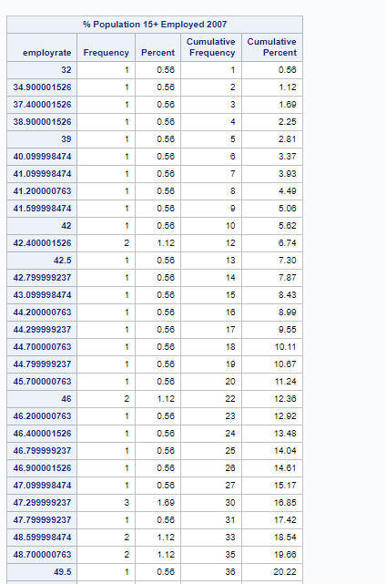
My last table is democracy score.

As this table is categorical, the whole table is included.

This table also had 52 missing values. All scores are from -10, the least democratic to 10, the mot democratic. Only 28.57% of countries have negative scores. And most of the denocratic countries have higher scores. 50% of the scores are 6 and above. This means that in general we live in a highly democratic world overall, despite some countries still facing autocratic rule.

python

I found python was a bit tricker in terms of its output not being as pretty. So at least in terms of frequency tables I have a preference for SAS over python in terms of the results being in a user friendly form.

Additionally, I used the internet to determine what some of my errors were in my first coding. For example I had to add “errors = coerce" when trying to convert my data to numeric.

I found that for my data, it was better to use the group by method as it sorted my data by value. However as a result it did not tell me how many NA’s there were. After a bit of research I found that by combining “isnull()” with “sum()” I could count my null values.

Here is my final code:

# load data data = pd.read_csv( 'D:/Users/jesnr/Dropbox/coursera/data management and visualization/gapminder data.csv', low_memory=(False))

# toprevent runtime errors #pd.set_option('display.float_format', lambda x: '%f'%x)

# print the frequency values and percentages feemprateval = data.groupby('femaleemployrate').size() feemprateper = data.groupby('femaleemployrate').size()*100/(len(data)-data['femaleemployrate'].isnull().sum())

print("count of % females 15 and over employed 2007") print(feemprateval) print("percentages of % females 15 and over employed 2007") print(feemprateper) print("missing values in female employment rate data") print(data['femaleemployrate'].isnull().sum()) print()

emprateval = data.groupby('employrate').size()emprateper = data.groupby('employrate').size()*100/(len(data)-data['employrate'].isnull().sum())

print("count of % population 15 and over employed 2007") print(emprateval) print("percentages of % population 15 and over employed 2007") print(emprateper) print("missing values in female employment rate data") print(data['employrate'].isnull().sum()) print()

dempval = data.groupby('polityscore').size() demper = data.groupby('polityscore').size()*100/(len(data)-data['polityscore'].isnull().sum())

print("count of % polity democracy score 2009") print(dempval) print("percentages of % polity democracy score 2009") print(demper) print("missing values in female employment rate data") print(data['polityscore'].isnull().sum()) print()

Please note that my analysis is identical to above because the numbers are all the same, as they should be. If they hadn’t been it would have indicated an error on my part

Now the tricky part here is that two of my data categories are continuous, so that makes these tables a bit long. Python agreed and truncated the output. So I have posted exactly what python outputted.On the continious data my descriptions will be based on the cumulative frequencies which i added up manually as most of the frequencies are just 1 or 2 data points and we were not taught how to do the cummulative frequencies yet.

So my first table is female empoyment rate.

count of % females 15 and over employed 2007 femaleemployrate 11.300000 1 12.400000 1 13.000000 1 16.700001 1 17.700001 1 .. 79.199997 1 80.000000 1 80.500000 1 82.199997 1 83.300003 1 Length: 153, dtype: int64 percentages of % females 15 and over employed 2007 femaleemployrate

11.300000 0.561798 12.400000 0.561798 13.000000 0.561798 16.700001 0.561798 17.700001 0.56179879.199997 0.561798 80.000000 0.561798 80.500000 0.561798 82.199997 0.561798 83.300003 0.561798

Length: 153, dtype: float64

missing values in female employment rate data 35

So my second table is overall empoyment rate.

count of % population 15 and over employed 2007 employrate 32.000000 1 34.900002 1 37.400002 1 38.900002 1 39.000000 1 .. 80.699997 1 81.300003 1 81.500000 1 83.000000 1 83.199997 2 Length: 139, dtype: int64 percentages of % population 15 and over employed 2007 employrate 332.000000 0.561798 34.900002 0.561798 37.400002 0.561798 38.900002 0.561798 39.000000 0.56179880.699997 0.561798 81.300003 0.561798 81.500000 0.561798 83.000000 0.561798 83.199997 1.123596 Length: 139, dtype: float64 missing values in female employment rate data 35

My last table is democracy score.

As this table is categorical, the whole table is included.

#data science #coursera

0 notes