meremaths

[meremaths]

\(\textbf{Bioelectrochemistry}\) \[\textit{Nernst Equation Example:}\] \[[K^{+}]\]

After having derived the Nernst equation,

\[V_{eq}=-\frac{RT}{Fz}ln\left[\frac{[C]_{in}}{[C]_{out}}\right]\]

Let us examine how it works. Say for example, in a human neuronal cell, the concentration of \(K^+\) ions outside the cell is \(5mM\), and inside is \(140mM\). The valence, \(z=1\). The equilibrium potential for this concentration gradient of this specific ion (i.e. when the diffusive and electrical potential across the membrane balance), is given by; \[V_{eq}=-26.7ln\frac{140}{5}\approx-89mV\]

When considering that the internal temperatures for biological activity is around \(37^{\circ}C\)

That is to say, at -89mV of potential difference across the cell membrane(the inside being more electronegative), there will be no net movement across the cell membrane for this ion.

[meremaths]

\(\textbf{Bioelectrochemistry}\) \[\textit{Nernst-Planck Equation}\]

We have, after obtaining the relationship between the diffusion constant, \(D\), and mobility, \(\mu\), the following expression for the total drift

\[J_{\Sigma}=- \frac{kT\mu}{q} \frac{\partial [C]}{\partial x}-\mu z [C] \frac{\partial V}{\partial x}\]

Let \(u\) be the molar mobility, such that

\[u=\frac{\mu}{A}\]

Where Avagadro’s constant, \(A\), is the number of particles in one mole. Faraday’s constant, \(F\) is the charge of one mole of electrons, where the charge of one electron is \(q\). \(zF\) is therefore the charge of one mole of homogenous ions with \(z\) being the nominal charge, or valence of the ion.

\[zF=zAq\]

Therefore

\[\mu z =uz^2F \]

The ideal gas constant, \(R\), which relates the kinetic energy of molecules to their temperature, is equivalent to the Boltzmann constant \(k\) for one mole of molecules

\[R=Ak\]

Therefore

\[\frac{kT\mu}{q}=\frac{uzFRT}{F}=uzRT\]

After these conversions, we can write the total flux equation, or the Nernst-Planck equation as follows

\[J_{\Sigma}=I=-\left( uzRT \frac{\partial [C]}{\partial x}+ uz^2F[C]\frac{\partial V}{\partial x}\right)\]

[meremaths]

\(\textbf{Physics}\) \[\textit{Diffusion Constant}\] \[\textit{& The Einstein Relation}\] \[D=kT\mu\]

We have seen the forms of diffusive drift and the electrical drift by Fick’s law and Ohm’s law, respectively. If we consider that no other external factors affect the movement of the particles, then at equilibrium

\[J_{diff}+J_{drift}=0\]

\[-D\frac{\partial [C]}{\partial x}-\mu z [C] \frac{\partial V}{\partial x}=0\]

If we consider the most general case of drift across a potential field, we may ignore the charge, such that \(z\) is redundant in this equation (\(z=1\)).

Remembering that this equation is satisfied at equilibrium where there is no net flow, and that the concentration of ions at a locality will depend only on the potential at that point, we can simplify this equation. In other words, at equilibrium, \([C]\) can be modelled as a function of \(V\). Therefore, by the chain rule;

\[\frac{\partial [C]}{\partial x} =\frac{d [C]}{dV}\frac{\partial V}{\partial x}\]

So that

\[ \frac{\partial V}{\partial x} \left(-D\frac{d[C]}{dV}-\mu [C]\right) =0\]

\[D = - \frac{\mu [C]}{\frac{d[C]}{dV}}\]

From Maxwell-Boltzmann Statistics [5], the concentration of the ions are distributed according to their energies (we assume that at equilibrium, the ions do not interact, so the energies are due only to potential)

\[[C]=ge^{-\frac{V}{kT}}\]

\[\frac{d[C]}{dV}=-g\frac{1}{kT} e^{-\frac{V}{kT}} = -\frac{1}{kT}[C]\]

Substituting this (naturally considering that \([C]\) is non-zero), we arrive at

\[D=kT\mu\]

This is the most general form for the diffusion constant. Notice how this value is directly proportional to the mobility. Since we know that both of these values are dependent on the diffusive material, this relation is quite useful.

In the specific case of cell membranes, the mobility used is also due to the ion, or in other words, we have the electrical mobility, \(\mu_q\)

\[\mu_q = \frac{\mu }{q}\]

So we have

\[D= \frac{kT\mu}{q} \]

Substituting this value into our equilibrium differential equation for cell membranes, we arrive at

\[- \frac{kT\mu}{q} \frac{\partial [C]}{\partial x}-\mu z [C] \frac{\partial V}{\partial x}=0\]

[meremaths]

\(\textbf{Physics}\) \[\textit{Microscopic Ohm’s Law}\]

The voltage between two points is directly proportional to the current between those points, states the traditional form of Ohm’s Law

\[V=IR\]

Where the constant of proportionality is termed ‘resistance’, and is a property of the conducting material. This is also termed as the ‘macroscopic Ohm’s Law’ and the observation can be made through relatively simple experimental procedure. For now, however, let’s explore this relation a little further.

Consider the potential difference across a cellular membrane, for example. Consider a current (an ion) passing across the membrane, then the small change in potential difference for every small amount it moves across the membrane is given by

\[E_x = \frac{\partial V}{\partial x}\]

Which tells us how the electrical field strength changes across the membrane (i.e. in the \(x\) direction).

At a point \(x\), say the charge density (ion concentration) is \([C]\), then the total charge should therefore be

\[z [C]\]

Where \(z\) is the nominal charge of a single ion (also known as valence). Therefore, the force on this charge, by the electrical field, is;

\[z [C] \frac{\partial V}{\partial x}\]

Ohm’s law states that the effective current, or \(\textit{drift}\) is proportional to the force exerted by the electrical (potential) field

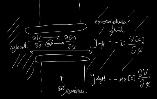
\[J_{drift} =- \mu z[C] \frac{\partial V}{\partial x}\]

Where \(\mu\) is the \(\textit{mobility}\) of the ion, which denotes the ease at which the ion moves across the material (membrane in this case).

Note that if we take a look at the direction of the ionic movement (from positive to negative), the change in field strength should oppose the direction of movement. Note also that the electrical mobility is a property of the ion and the conducting material. Intuitively, this term therefore serves as the replacement for \(R\) in the macroscopic Ohm’s Law.

[meremaths]

\(\textbf{Chemistry}\) \[\textit{Fick’s Law of Diffusion}\]

Consider diffusion. It is the movement of particles from higher concentrations to lower concentrations. Consider a one-dimensional movement of ions across a cell membrane from regions where the concentration is higher to regions where it is lower across the concentration gradient. In other words, the \(\textit{diffusive flux}\), \( J_{diff} \) is equivalent to some scale of the concentration gradient.

\[J_{diff} \propto \frac{d[C]}{dx} \]

Where \(x\) is the position along the concentration gradient and \([C]\) is the concentration at that point.

This is known as Fick’s first law of diffusion in the most ideal scenario. It is a relatively simple concept, taken from the idea that diffusion depends, and is proportional to, the degree of magnitude of the concentration gradient. \(J_{diff}\) is given in the amount of substance per unit area per unit time.

Of course, the other value which \( J_{diff}\) depends upon is the substance itself. The diffusivity of a substance is how easy or difficult it is for the substance to diffuse, given its chemical properties such as mass and viscosity. We thus term \(D\) the diffusion constant of a substance with dimensions of area per second.

Lastly, since the movement is in the negative direction (from high to low), a negative sign must be multiplied.

\[J_{diff}=-D\frac{d[C]}{dx}\]

Typically speaking, the derivatives in this equation would be partial ones due to the other spatial dimensions which may determine the concentration in a given space. In this case, we simply take partial derivatives along each of the axes.

However, when looking at diffusion across a cell membrane, we are only considering diffusion in one specific direction (perpendicular to the membrane in the path joining the inside and outside of the cell), \(x\), say, such that

\[J_{diff}=-D\frac{\partial [C]}{\partial x}\]

[meremaths]

\(\textbf{Neurophysiology}\) \[\textit{The Hodgkin-Huxley Model}\] \[\textit{Part 1 - Nernst Equation}\] \[V_{eq}=-\frac{RT}{zF}ln\frac{[C_{in}]}{[C_{out}]}\]

The Hodgkin-Huxley model for neuronal activity is one of the most well studied. It is also the inspiration for the perceptron and neural network models found in machine learning algorithms of today. More than that however, it was one of our first insights into a physiological mechanism, which to this day, is still in the process of being unraveled.

In explaining the fundamentals of this model, we will walk along a winding road full of neat and often clever mathematical descriptions which will inevitably build upon each other until we arrive at our destination. The first stop, per the title, is the Nernst Equation.

The \(\textit{membrane potential}\) of a cell, is the potential difference between the inside and outside of a cell across its membrane.

\[V_m=V_{in}-V_{out}\]

The \(\textit{resting potential}\) is the potential across the cellular membrane when the cell is at rest, with the inside being more electronegative. The typical value for a neuron is \(-70mV\).

The \(\textit{equiibrium potential}\) across a membrane for a particular ion is the potential at which the electrical and diffusive movement are equal and opposite, such that there is no net movement across the membrane for that ion. The following relation must therefore be satisfied

\[J_{diff} + J_{drift} = 0\]

From Fick’s law [1]:

\[J_{diff} \propto \frac{\partial [C]}{\partial x}\]

From Ohm’s Law [2]:

\[J_{drift} \propto z[C]\frac{\partial V}{\partial x}\]

Where \([C]\) is the concentration, and \(V\) is the potential of the given ion at the point \(x\) across the membrane.

It is found by the Einstein relation [3] that, adjusting the coefficients of these terms and summating them, we arrive at the Nernst-Planck equation [4]; an expression for the \(\textit{current flux}\), \(I\)

\[I=-uzRT\frac{\partial [C]}{\partial x}-uz^2F[C]\frac{\partial V}{\partial x}\]

At \(I=0\), we can evaluate the equilibrium potential for ions passing through an open channel by solving the differential equation

\[-uzRT\frac{\partial [C]}{\partial x}-uz^2F[C]\frac{\partial V}{\partial x} =0\]

\[\frac{\partial V}{\partial x} = -\frac{RT}{Fz}\frac{1}{[C]}\frac{\partial [C]}{\partial x}\]

Summating over the domain (from \(x=0\) to \(x=l\), where  \(l\) is the thickness of the membrane), which is from the inside to the outside of the cell, we arrive at

\[\int_{out}^{in}VdV=-\frac{RT}{Fz}\int_{out}^{in}\frac{1}{[C]}d[C]\]

\[V_{eq}=-\frac{RT}{Fz}ln\frac{[C_{in}]}{[C_{out}]}\]

This equation provides the equilibrium potential given a concentration gradient of ions across an open channel.

This equation assumes that the ions do not interact, and that the medium of the flux is aqueous. Typically, cell membranes behave in a more complex way, however, deriving this equation is a good start for a simplified model.