pabloatech

[pabloatech]

4th week: plotting variables

I put here as usual the python script, the results and the comments:

Python script:

Created on Tue Jun 3 09:06:33 2025

@author: PabloATech """

libraries/packages

import pandas import numpy import seaborn import matplotlib.pyplot as plt

read the csv table with pandas:

data = pandas.read_csv('C:/Users/zop2si/Documents/Statistic_tests/nesarc_pds.csv', low_memory=False)

show the dimensions of the data frame:

print() print ("length of the dataframe (number of rows): ", len(data)) #number of observations (rows) print ("Number of columns of the dataframe: ", len(data.columns)) # number of variables (columns)

variables:

variable related to the background of the interviewed people (SES: socioeconomic status):

biological/adopted parents got divorced or stop living together before respondant was 18

data['S1Q2D'] = pandas.to_numeric(data['S1Q2D'], errors='coerce')

variable related to alcohol consumption

HOW OFTEN DRANK ENOUGH TO FEEL INTOXICATED IN LAST 12 MONTHS

data['S2AQ10'] = pandas.to_numeric(data['S2AQ10'], errors='coerce')

variable related to the major depression (low mood I)

EVER HAD 2-WEEK PERIOD WHEN FELT SAD, BLUE, DEPRESSED, OR DOWN MOST OF TIME

data['S4AQ1'] = pandas.to_numeric(data['S4AQ1'], errors='coerce')

NUMBER OF EPISODES OF PATHOLOGICAL GAMBLING

data['S12Q3E'] = pandas.to_numeric(data['S12Q3E'], errors='coerce')

HIGHEST GRADE OR YEAR OF SCHOOL COMPLETED

data['S1Q6A'] = pandas.to_numeric(data['S1Q6A'], errors='coerce')

Choice of thee variables to display its frequency tables:

string_01 = """ Biological/adopted parents got divorced or stop living together before respondant was 18: 1: yes 2: no 9: unknown -> deleted from the analysis blank: unknown """

string_02 = """ HOW OFTEN DRANK ENOUGH TO FEEL INTOXICATED IN LAST 12 MONTHS

Every day

Nearly every day

3 to 4 times a week

2 times a week

Once a week

2 to 3 times a month

Once a month

7 to 11 times in the last year

3 to 6 times in the last year

1 or 2 times in the last year

Never in the last year

Unknown -> deleted from the analysis BL. NA, former drinker or lifetime abstainer """

string_02b = """ HOW MANY DAYS DRANK ENOUGH TO FEEL INTOXICATED IN THE LAST 12 MONTHS: """

string_03 = """ EVER HAD 2-WEEK PERIOD WHEN FELT SAD, BLUE, DEPRESSED, OR DOWN MOST OF TIME:

Yes

No

Unknown -> deleted from the analysis """

string_04 = """ NUMBER OF EPISODES OF PATHOLOGICAL GAMBLING """

string_05 = """ HIGHEST GRADE OR YEAR OF SCHOOL COMPLETED

No formal schooling

Completed grade K, 1 or 2

Completed grade 3 or 4

Completed grade 5 or 6

Completed grade 7

Completed grade 8

Some high school (grades 9-11)

Completed high school

Graduate equivalency degree (GED)

Some college (no degree)

Completed associate or other technical 2-year degree

Completed college (bachelor's degree)

Some graduate or professional studies (completed bachelor's degree but not graduate degree)

Completed graduate or professional degree (master's degree or higher) """

replace unknown values for NaN and remove blanks

data['S1Q2D']=data['S1Q2D'].replace(9, numpy.nan) data['S2AQ10']=data['S2AQ10'].replace(99, numpy.nan) data['S4AQ1']=data['S4AQ1'].replace(9, numpy.nan) data['S12Q3E']=data['S12Q3E'].replace(99, numpy.nan) data['S1Q6A']=data['S1Q6A'].replace(99, numpy.nan)

create a recode for number of intoxications in the last 12 months:

recode1 = {1:365, 2:313, 3:208, 4:104, 5:52, 6:36, 7:12, 8:11, 9:6, 10:2, 11:0} data['S2AQ10'] = data['S2AQ10'].map(recode1)

print(" ") print("Statistical values for varible 02 alcohol intoxications of past 12 months") print(" ") print ('mode: ', data['S2AQ10'].mode()) print ('mean', data['S2AQ10'].mean()) print ('std', data['S2AQ10'].std()) print ('min', data['S2AQ10'].min()) print ('max', data['S2AQ10'].max()) print ('median', data['S2AQ10'].median()) print(" ") print("Statistical values for highest grade of school completed") print ('mode', data['S1Q6A'].mode()) print ('mean', data['S1Q6A'].mean()) print ('std', data['S1Q6A'].std()) print ('min', data['S1Q6A'].min()) print ('max', data['S1Q6A'].max()) print ('median', data['S1Q6A'].median()) print(" ")

plot01 = seaborn.countplot(x="S2AQ10", data=data) plt.xlabel('Alcohol intoxications past 12 months') plt.title('Alcohol intoxications in the Past 12 Months in the NESARC Study')

plot02 = seaborn.countplot(x="S1Q6A", data=data) plt.xlabel('Highest grade (1-14)') plt.title('Highest grade or year of school completed')

I create a copy of the data to be manipulated later

sub1 = data[['S2AQ10','S1Q6A']]

create bins for no intoxication, few intoxications, …

data['S2AQ10'] = pandas.cut(data.S2AQ10, [0, 6, 36, 52, 104, 208, 365], labels=["very few","some", "often", "quite often", "very often", "permanent"])

change format from numeric to categorical

data['S2AQ10'] = data['S2AQ10'].astype('category')

print ('intoxication category counts') c1 = data['S2AQ10'].value_counts(sort=False, dropna=True) print(c1)

bivariate bar graph C->Q

plot03 = seaborn.catplot(x="S2AQ10", y="S1Q6A", data=data, kind="bar", ci=None) plt.xlabel('Alcohol intoxications') plt.ylabel('Highest grade')

c4 = data['S1Q6A'].value_counts(sort=False, dropna=False) print("c4: ", c4) print(" ")

I do sth similar but the way around:

creating 3 level education variable

def edu_level_1 (row): if row['S1Q6A'] <9 : return 1 # high school if row['S1Q6A'] >8 and row['S1Q6A'] <13 : return 2 # bachelor if row['S1Q6A'] >12 : return 3 # master or higher

sub1['edu_level_1'] = sub1.apply (lambda row: edu_level_1 (row),axis=1)

change format from numeric to categorical

sub1['edu_level'] = sub1['edu_level'].astype('category')

plot04 = seaborn.catplot(x="edu_level_1", y="S2AQ10", data=sub1, kind="boxen") plt.ylabel('Alcohol intoxications in the past 12 months') plt.xlabel('Highest grade') plt.grid() plt.show()

Results and comments:

length of the dataframe (number of rows): 43093 Number of columns of the dataframe: 3008

Statistical values for variable "alcohol intoxications of past 12 months":

mode: 0 0.0 dtype: float64 mean 9.115493905630748 std 40.54485720135516 min 0.0 max 365.0 median 0.0

Statistical values for variable "highest grade of school completed":

mode 0 8 dtype: int64 mean 9.451024528345672 std 2.521281770664422 min 1 max 14 median 10.0

intoxication category counts very few 6026 some 2042 often 510 quite often 272 very often 184 permanent 276 Name: S2AQ10, dtype: int64

c4: (counts highest grade)

8 10935 6 1210 12 5251 14 3257 10 8891 13 1526 7 4518 11 3772 5 414 4 931 3 421 9 1612 2 137 1 218 Name: S1Q6A, dtype: int64

Plots: Univariate highest grade:

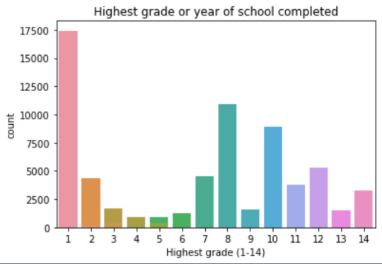
mean 9.45 std 2.5

-> mean and std. dev. are not very useful for this category-distribution. Most interviewed didn´t get any formal schooling, the next larger group completed the high school and the next one was at some college but w/o degree.

Univariate number of alcohol intoxications:

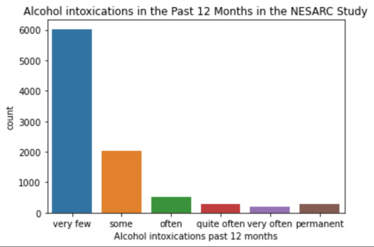
mean 9.12 std 40.54

-> very left skewed, most of the interviewed persons didn´t get intoxicated at all or very few times in the last 12 months (as expected)

Bivariate: the one against the other:

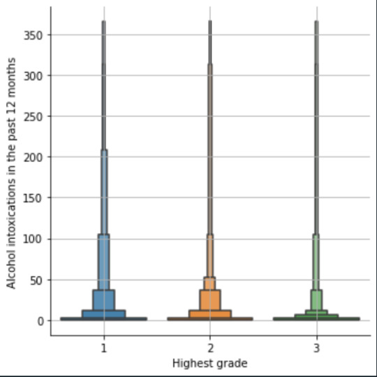
This bivariate plot shows three categories:

1: high school or lower

2: high school to bachelor

3: master or PhD

And the frequency of alcohol intoxications in the past 12 months.

The number of intoxications is higher in the group 1 for all the segments, but from 1 to 3 every group shows occurrences in any number of intoxications. More information and a more detailed analysis would be necessary to make conclusions.

[pabloatech]

Week 3:

I put here the script, the results and its description:

PYTHON:

Created on Thu May 22 14:21:21 2025

@author: Pablo """

libraries/packages

import pandas import numpy

read the csv table with pandas:

data = pandas.read_csv('C:/Users/zop2si/Documents/Statistic_tests/nesarc_pds.csv', low_memory=False)

show the dimensions of the data frame:

print() print ("length of the dataframe (number of rows): ", len(data)) #number of observations (rows) print ("Number of columns of the dataframe: ", len(data.columns)) # number of variables (columns)

variables:

variable related to the background of the interviewed people (SES: socioeconomic status):

biological/adopted parents got divorced or stop living together before respondant was 18

data['S1Q2D'] = pandas.to_numeric(data['S1Q2D'], errors='coerce')

variable related to alcohol consumption

HOW OFTEN DRANK ENOUGH TO FEEL INTOXICATED IN LAST 12 MONTHS

data['S2AQ10'] = pandas.to_numeric(data['S2AQ10'], errors='coerce')

variable related to the major depression (low mood I)

EVER HAD 2-WEEK PERIOD WHEN FELT SAD, BLUE, DEPRESSED, OR DOWN MOST OF TIME

data['S4AQ1'] = pandas.to_numeric(data['S4AQ1'], errors='coerce')

Choice of thee variables to display its frequency tables:

string_01 = """ Biological/adopted parents got divorced or stop living together before respondant was 18: 1: yes 2: no 9: unknown -> deleted from the analysis blank: unknown """

string_02 = """ HOW OFTEN DRANK ENOUGH TO FEEL INTOXICATED IN LAST 12 MONTHS

Every day

Nearly every day

3 to 4 times a week

2 times a week

Once a week

2 to 3 times a month

Once a month

7 to 11 times in the last year

3 to 6 times in the last year

1 or 2 times in the last year

Never in the last year

Unknown -> deleted from the analysis BL. NA, former drinker or lifetime abstainer """

string_02b = """ HOW MANY DAYS DRANK ENOUGH TO FEEL INTOXICATED IN THE LAST 12 MONTHS:

"""

string_03 = """ EVER HAD 2-WEEK PERIOD WHEN FELT SAD, BLUE, DEPRESSED, OR DOWN MOST OF TIME:

Yes

No

Unknown -> deleted from the analysis """

replace unknown values for NaN and remove blanks

data['S1Q2D']=data['S1Q2D'].replace(9, numpy.nan) data['S2AQ10']=data['S2AQ10'].replace(99, numpy.nan) data['S4AQ1']=data['S4AQ1'].replace(9, numpy.nan)

create a subset to know how it works

sub1 = data[['S1Q2D','S2AQ10','S4AQ1']]

create a recode for yearly intoxications:

recode1 = {1:365, 2:313, 3:208, 4:104, 5:52, 6:36, 7:12, 8:11, 9:6, 10:2, 11:0} sub1['Yearly_intoxications'] = sub1['S2AQ10'].map(recode1)

create the tables:

print() c1 = data['S1Q2D'].value_counts(sort=True) # absolute counts

print (c1)

print(string_01) p1 = data['S1Q2D'].value_counts(sort=False, normalize=True) # percentage counts print (p1)

c2 = sub1['Yearly_intoxications'].value_counts(sort=False) # absolute counts

print (c2)

print(string_02b) p2 = sub1['Yearly_intoxications'].value_counts(sort=True, normalize=True) # percentage counts print (p2) print()

c3 = data['S4AQ1'].value_counts(sort=False) # absolute counts

print (c3)

print(string_03) p3 = data['S4AQ1'].value_counts(sort=True, normalize=True) # percentage counts print (p3)

RESULTS:

Biological/adopted parents got divorced or stop living together before respondant was 18: 1: yes 2: no 9: unknown -> deleted from the analysis blank: unknown

2.0 0.814015 1.0 0.185985 Name: S1Q2D, dtype: float64

HOW MANY DAYS DRANK ENOUGH TO FEEL INTOXICATED IN THE LAST 12 MONTHS:

0.0 0.651911 2.0 0.162118 6.0 0.063187 12.0 0.033725 11.0 0.022471 36.0 0.020153 52.0 0.019068 104.0 0.010170 208.0 0.006880 365.0 0.006244 313.0 0.004075 Name: Yearly_intoxications, dtype: float64

EVER HAD 2-WEEK PERIOD WHEN FELT SAD, BLUE, DEPRESSED, OR DOWN MOST OF TIME:

Yes

No

Unknown -> deleted from the analysis

2.0 0.697045 1.0 0.302955 Name: S4AQ1, dtype: float64

Description:

In regard to computing: the unknown answers were substituted by nan and therefore not considered for the analysis. The original responses to the number of yearly intoxications, which were not a direct figure, were transformed by mapping to yield the actual number of yearly intoxications. For doing this, a submodel was also created.

In regard to the content:

The first variable is quite simple: 18,6% of the respondents saw their parents divorcing before they were 18 years old.

The second variable is the number of yearly intoxications. The highest frequency is as expected not a single intoxication in the last 12 months (65,19%). The more the number of intoxications, the smaller the probability, with an only exception: 0,6% got intoxicated every day and 0,4% got intoxicated almost everyday. I would have expected this numbers flipped.

The last variable points a relatively high frequency of people going through periods of sadness: 30,29%. However, it isn´t yet enough to classify all these periods of sadness as low mood or major depression. A further analysis is necessary.

[pabloatech]

Frequency tables for selected variables

I post here the python script, the results and the comments:

Python script:

libraries/packages

import pandas import numpy

read the csv table with pandas:

data = pandas.read_csv('C:/Users/zop2si/Documents/Statistic_tests/nesarc_pds.csv', low_memory=False)

show the dimensions of the data frame:

print() print ("length of the dataframe (number of rows): ", len(data)) #number of observations (rows) print ("Number of columns of the dataframe: ", len(data.columns)) # number of variables (columns)

variables:

variables related to the background of the interviewed people (SES: socioeconomic status):

building type

data['BUILDTYP'] = pandas.to_numeric(data['BUILDTYP'], errors='coerce')

number of persons in the household

data['NUMPERS'] = pandas.to_numeric(data['NUMPERS'], errors='coerce')

number of persons older than 18 years in the household

data['NUMPER18'] = pandas.to_numeric(data['NUMPER18'], errors='coerce')

year of birth

data['DOBY'] = pandas.to_numeric(data['DOBY'], errors='coerce')

biological/adopted parents got divorced or stop living together before respondant was 18

data['S1Q2D'] = pandas.to_numeric(data['S1Q2D'], errors='coerce')

marital status

data['MARITAL'] = pandas.to_numeric(data['MARITAL'], errors='coerce')

number of marriages

data['S1Q3B'] = pandas.to_numeric(data['S1Q3B'], errors='coerce')

highest grade or year of school completed

data['S1Q6A'] = pandas.to_numeric(data['S1Q6A'], errors='coerce')

variables related to alcohol consumption

HOW OFTEN DRANK COOLERS IN LAST 12 MONTHS

data['S2AQ4B'] = pandas.to_numeric(data['S2AQ4B'], errors='coerce')

HOW OFTEN DRANK 5+ COOLERS IN LAST 12 MONTHS

data['S2AQ4G'] = pandas.to_numeric(data['S2AQ4G'], errors='coerce')

HOW OFTEN DRANK BEER IN LAST 12 MONTHS

data['S2AQ5B'] = pandas.to_numeric(data['S2AQ5B'], errors='coerce')

NUMBER OF BEERS USUALLY CONSUMED ON DAYS WHEN DRANK BEER IN LAST 12 MONTHS

data['S2AQ5D'] = pandas.to_numeric(data['S2AQ5D'], errors='coerce')

HOW OFTEN DRANK 5+ BEERS IN LAST 12 MONTHS

data['S2AQ5G'] = pandas.to_numeric(data['S2AQ5G'], errors='coerce')

HOW OFTEN DRANK WINE IN LAST 12 MONTHS

data['S2AQ6B'] = pandas.to_numeric(data['S2AQ6B'], errors='coerce')

NUMBER OF GLASSES/CONTAINERS OF WINE USUALLY CONSUMED ON DAYS WHEN DRANK WINE IN LAST 12 MONTHS

data['S2AQ6D'] = pandas.to_numeric(data['S2AQ6D'], errors='coerce')

HOW OFTEN DRANK 5+ GLASSES/CONTAINERS OF WINE IN LAST 12 MONTHS

data['S2AQ6G'] = pandas.to_numeric(data['S2AQ6G'], errors='coerce')

HOW OFTEN DRANK ENOUGH TO FEEL INTOXICATED IN LAST 12 MONTHS

data['S2AQ10'] = pandas.to_numeric(data['S2AQ10'], errors='coerce')

variables relatred to personality disorder: low mood (dysthemia) or major depression

AGE AT ONSET OF ALCOHOL DEPENDENCE

data['ALCABDEP12DX'] = pandas.to_numeric(data['ALCABDEP12DX'], errors='coerce')

0: No alcohol dependence

1: Alcohol abuse

2: Alcohol dependence

3: Alcohol abuse and dependence

variables related to the major depression (low mood I)

EVER HAD 2-WEEK PERIOD WHEN FELT SAD, BLUE, DEPRESSED, OR DOWN MOST OF TIME

data['S4AQ1'] = pandas.to_numeric(data['S4AQ1'], errors='coerce')

EVER HAD 2-WEEK PERIOD WHEN DIDN'T CARE ABOUT THINGS USUALLY CARED ABOUT

data['S4AQ2'] = pandas.to_numeric(data['S4AQ2'], errors='coerce')

FELT TIRED/EASILY TIRED NEARLY EVERY DAY FOR 2+ WEEKS, WHEN NOT DOING MORE THAN USUAL

data['S4AQ4A8'] = pandas.to_numeric(data['S4AQ4A8'], errors='coerce')

FELT WORTHLESS MOST OF THE TIME FOR 2+ WEEKS

data['S4AQ4A12'] = pandas.to_numeric(data['S4AQ4A12'], errors='coerce')

FELT GUILTY ABOUT THINGS WOULDN'T NORMALLY FEEL GUILTY ABOUT 2+ WEEKS

data['S4AQ4A13'] = pandas.to_numeric(data['S4AQ4A13'], errors='coerce')

FELT UNCOMFORTABLE OR UPSET BY LOW MOOD OR THESE OTHER EXPERIENCES

data['S4AQ51'] = pandas.to_numeric(data['S4AQ51'], errors='coerce')

Choice of thee variables to display its frequency tables:

string_01 = """ Biological/adopted parents got divorced or stop living together before respondant was 18: 1: yes 2: no 9: unknown blank: unknown """

replace unknown values for NaN and remove blanks

data['S1Q2D']=data['S1Q2D'].replace(9, numpy.nan)

data['S1Q2D']=data['S1Q2D'].dropna

string_02 = """ HOW OFTEN DRANK ENOUGH TO FEEL INTOXICATED IN LAST 12 MONTHS

Every day

Nearly every day

3 to 4 times a week

2 times a week

Once a week

2 to 3 times a month

Once a month

7 to 11 times in the last year

3 to 6 times in the last year

1 or 2 times in the last year

Never in the last year

Unknown BL. NA, former drinker or lifetime abstainer """

replace unknown values for NaN and remove blanks

data['S2AQ10']=data['S2AQ10'].replace(99, numpy.nan)

data['S2AQ10']=data['S2AQ10'].dropna

string_03 = """ EVER HAD 2-WEEK PERIOD WHEN FELT SAD, BLUE, DEPRESSED, OR DOWN MOST OF TIME:

Yes

No

Unknown """

replace unknown values for NaN and remove blanks

data['S2AQ1']=data['S2AQ1'].replace(99, numpy.nan)

data['S2AQ1']=data['S2AQ1'].dropna

create the tables:

print() c1 = data['S1Q2D'].value_counts(sort=False) # absolute counts

print (c1)

print(string_01) p1 = data['S1Q2D'].value_counts(sort=False, normalize=True) # percentage counts print (p1)

c2 = data['S2AQ10'].value_counts(sort=False) # absolute counts

print (c2)

print(string_02) p2 = data['S2AQ10'].value_counts(sort=False, normalize=True) # percentage counts print (p2) print()

c3 = data['S2AQ1'].value_counts(sort=False) # absolute counts

print (c3)

print(string_03) p3 = data['S2AQ1'].value_counts(sort=False, normalize=True) # percentage counts print (p3)

Results:

length of the dataframe (number of rows): 43093 Number of columns of the dataframe: 3008

Biological/adopted parents got divorced or stop living together before respondant was 18: 1: yes 2: no 9: unknown blank: unknown

2.000000 0.812594 1.000000 0.185661 9.000000 0.001745 Name: S1Q2D, dtype: float64

HOW OFTEN DRANK ENOUGH TO FEEL INTOXICATED IN LAST 12 MONTHS

Every day

Nearly every day

3 to 4 times a week

2 times a week

Once a week

2 to 3 times a month

Once a month

7 to 11 times in the last year

3 to 6 times in the last year

1 or 2 times in the last year

Never in the last year

Unknown BL. NA, former drinker or lifetime abstainer

11.000000 0.647072 10.000000 0.160914 9.000000 0.062718 8.000000 0.022304 7.000000 0.033474 5.000000 0.018927 1.000000 0.006198 6.000000 0.020003 3.000000 0.006828 2.000000 0.004045 4.000000 0.010094 99.000000 0.007422 Name: S2AQ10, dtype: float64

EVER HAD 2-WEEK PERIOD WHEN FELT SAD, BLUE, DEPRESSED, OR DOWN MOST OF TIME:

Yes

No

Unknown

2 0.191818 1 0.808182 Name: S2AQ1, dtype: float64

Comments:

It is too early to make any conclusions without further statistical analysis.

In regard to the computing: the sort function of pandas eliminates by default the nan values and blank cells, therefore the percentages are referred to the sum of cells with a numerical value within.

In regard to the content:

One interesting thing is the amount of people that felt sad, blue, depressed or down most of the time for a period over two weeks (80,81%). More variables would be necessary in order to find out the depth of these mood states.

Another interesting fact is that almost 35% of the interviewed people felt intoxicated by alcohol consumption at least once in the last 12 months. That is a high figure.

Finally, it is remarkable that although the divorce rates are very high, only 18,57% of the interviewed individuals reported parents divorcing or living separately before they were 18 years old.

[pabloatech]

My research project

Data set: NESARC

I am interested in the alcohol dependence, its possible causes and its effects on the personality (personal disorders). Since I don´t know by now what variables may be relevant, I would include section 1 (background), section 2 (alcohol), section 4 for the effects (low mood to major depression).

My research question is oriented to the statistical relevance of alcohol consumption and/or dependence in the population with personality disorders, e. g. low mood (dysthimia) or major depression.

Additionally, as an additional research question, it would be interesting to check the dependance of alcohol consumption upon background information such as the socioeconomical environment (e. g. divorced parents). The information for doing it is included in the section 1.

A search in scholar.google.com for the term "relationship between alcohol and depression" produces 3,5 million results. It seems to be an interesting research topic. By filtering the search results by date of publication "since 2021", the results list still include 60800 results.

This research topic has been studied from multiple points of view, hereby some of them:

-> Influence of genes and alcohol consumption/smoking on anxiety and depression: Yang, Xuena, et al. "Evaluating the interaction between 3'aQTL and alcohol consumption/smoking on anxiety and depression: 3'aQTL-by-environment interaction study in UK Biobank cohort." Journal of Affective Disorders 338 (2023): 518-525. Results:anxiety score and depression are positively associated to some genes and to the alcohol abuse.

-> Influence of heavy alcohol consumption and all-cause mortality: Yan, C., Ding, Y., He, H. et al. Heavy alcohol consumption, depression, their comorbidity and risk of all-cause and cause-specific mortality: a prospective cohort study. Soc Psychiatry Psychiatr Epidemiol (2025). https://doi.org/10.1007/s00127-025-02873-9 Results: Heavy alcohol consumption or depression was associated with an increased risk of all-cause and other-cause mortality.

-> Influence of alcohol consumption on anxiety and depression of health care workers: Edgar Omar Vázquez-Puente, Karla Selene López-García, Francisco Rafael, Guzmán-Facundo, Ramón Valladares-Trujillo, Adriana Patricia Castillo-Méndez. Anxiety and Depressive Symptoms Associated to Alcohol Consumption in Health Care Workers. Horizon Interdisciplinary Journal (HIJ). ISSN: 2992-7706 Volume 1 (3): e14. October-December. 2023.

I chose one article for a deeper review:

Aurélie M. Lasserre, Sameer Imtiaz, Michael Roerecke, Markus Heilig, Charlotte Probst, Jürgen Rehm, Socioeconomic status, alcohol use disorders, and depression: A population-based study, Journal of Affective Disorders, Volume 301, 2022, Pages 331-336, ISSN 0165-0327, https://doi.org/10.1016/j.jad.2021.12.132. (https://www.sciencedirect.com/science/article/pii/S016503272101452X)

My findings from the conducted study and its result:

The data set used for this study is the same NESCAR Wave 1 that is available with this Coursera course!

Variables considered: AUD (alchohol use disorder) distributed in several categories; SES (socioeconomic status) based on the educational attainment; race/ethnicity and of course DD (depressive disorders).

Summary: The study results provide evidence with a unidirectional causal relationship between AUD and subsequent DD: The risk of developing an incident DD increased gradually with the recency and the severity of AUD at baseline, but the converse was not observed. Moreover, a low SES was an independent risk factor for incident DD and for incident AUD, and the strength of the association between AUD and DD did not vary between low or high SES.

Limitations: At the end of the study, some limitations are named: Craving (not included in the interviews) - Missing the craving criteria could have led to an underestimation of the AUD severity Time frame: his survey was conducted in the first decade of the 21st century, prior to the decrease in life expectancy due to “deaths of despair”. No information about adverse childhood events or other traumatic experiences at baseline Anxiety disorders or cigarette smoking weren´t included in the models, despite their possible association with AUD and DD.

All in all, an interesting research topic to learn about!

[pabloatech]

Beerdays in a year depending on divorce of parents and moderated by sex

I run an anova for the quantitative variable "days a year beer is consumed" related to the categorical variable "parents divorced before respondant was 18 years old". There was no significant relevance for the categorical explanation. However, by introducing a moderator as the respondent sex (male/female), the categorical variable became relevant for the female respondents (p-value 0.0259<0.05).

Here you can see the python code:

import numpy import pandas import statsmodels.formula.api as smf

import statsmodels.stats.multicomp as multi

data = pandas.read_csv('C:/Users/zop2si/Documents/Statistic_tests/nesarc_pds.csv', low_memory=False)

convert data to numeric

data['S2AQ5B'] = pandas.to_numeric(data['S2AQ5B'], errors='coerce') # quantitative variable: how often drank beer in the last 12 months data['S1Q2D'] = pandas.to_numeric(data['S1Q2D'], errors='coerce') # categorical variable: parents got divorced before respondent was 18

subset adults age older than 18

sub1=data[data['AGE']>=18]

SETTING MISSING DATA

sub1['S2AQ5B']=sub1['S2AQ5B'].replace(99, numpy.nan) sub1['S1Q2D']=sub1['S1Q2D'].replace(9, numpy.nan)

recoding number of days when beer was drunk according to the nesarc documentation

recode1 = {1: 365, 2: 330, 3: 208, 4: 104, 5: 52, 6: 36, 7: 12, 8:11, 9: 6, 10: 2} sub1['BEERDAY']= sub1['S2AQ5B'].map(recode1)

converting new variable to numeric

sub1['BEERDAY']= pandas.to_numeric(sub1['BEERDAY'], errors='coerce')

ct1 = sub1.groupby('BEERDAY').size() print("Values in ct1 grouped by size of factor: ") print (ct1)

using ols function for calculating the F-statistic and associated p value

model1 = smf.ols(formula='BEERDAY ~ C(S1Q2D)', data=sub1) results1 = model1.fit() print (results1.summary())

drop empty rows from the model:

sub2 = sub1[['BEERDAY', 'S1Q2D']].dropna()

print(" ") print ('means for beerday by highest degree') m1= sub2.groupby('S1Q2D').mean() print (m1)

print(" ") print ('standard deviations for beerday by highest degree') sd1 = sub2.groupby('S1Q2D').std() print (sd1) print(" ") print(" ")

Check with the moderator parameter "sex"

sub11=data[(data['SEX']==1)] sub12=data[(data['SEX']==2)]

SETTING MISSING DATA

sub11['S2AQ5B']=sub11['S2AQ5B'].replace(99, numpy.nan) sub11['S1Q2D']=sub11['S1Q2D'].replace(9, numpy.nan) sub12['S2AQ5B']=sub12['S2AQ5B'].replace(99, numpy.nan) sub12['S1Q2D']=sub12['S1Q2D'].replace(9, numpy.nan)

recoding number of days when beer was drunk according to the nesarc documentation

recode1 = {1: 365, 2: 330, 3: 208, 4: 104, 5: 52, 6: 36, 7: 12, 8:11, 9: 6, 10: 2} sub11['BEERDAY']= sub11['S2AQ5B'].map(recode1) sub12['BEERDAY']= sub12['S2AQ5B'].map(recode1)

converting new variable to numeric

sub11['BEERDAY']= pandas.to_numeric(sub11['BEERDAY'], errors='coerce') sub12['BEERDAY']= pandas.to_numeric(sub12['BEERDAY'], errors='coerce')

print(" ") print ('association between BEERDAY, divorced parents before age of 18 and male sex') model2 = smf.ols(formula='BEERDAY ~ C(S1Q2D)', data=sub11).fit() print (model2.summary()) print(" ") print ('association between BEERDAY, divorced parents before age of 18 and female sex') model3 = smf.ols(formula='BEERDAY ~ C(S1Q2D)', data=sub12).fit() print (model3.summary())

create subsets for male and female to show the mean and std. deviation

m101 = sub11[['BEERDAY','S1Q2D']] m102 = sub12[['BEERDAY','S1Q2D']]

print(" ") print ("Means for BEERDAY for divorced parents (S1Q2D=1) or not (S1Q2D=1) for males") m3= m101.groupby('S1Q2D').mean() print (m3) print ("Std. dev. for BEERDAY for divorced parents (S1Q2D=1) or not (S1Q2D=1) for males") m31= m101.groupby('S1Q2D').std() print (m31) print(" ") print ("Means for BEERDAY for divorced parents (S1Q2D=1) or not (S1Q2D=1) for females") m4 = m102.groupby('S1Q2D').mean() print (m4) print ("Std. dev. for BEERDAY for divorced parents (S1Q2D=1) or not (S1Q2D=1) for females") m41 = m102.groupby('S1Q2D').std() print (m41)

Results:

OLS Regression Results

Dep. Variable: BEERDAY R-squared: 0.000 Model: OLS Adj. R-squared: 0.000 Method: Least Squares F-statistic: 1.739 Date: Wed, 14 May 2025 Prob (F-statistic): 0.187 Time: 07:23:34 Log-Likelihood: -97052. No. Observations: 16123 AIC: 1.941e+05 Df Residuals: 16121 BIC: 1.941e+05 Df Model: 1

Covariance Type: nonrobust

coef std err t P>|t| [0.025 0.975]

Intercept 74.6835 1.708 43.727 0.000 71.336 78.031

C(S1Q2D)[T.2.0] -2.5351 1.922 -1.319 0.187 -6.303 1.233

Omnibus: 5083.122 Durbin-Watson: 2.003 Prob(Omnibus): 0.000 Jarque-Bera (JB): 12184.626 Skew: 1.809 Prob(JB): 0.00 Kurtosis: 5.247 Cond. No. 4.15

association between BEERDAY, divorced parents before age of 18 and male sex

OLS Regression Results

Dep. Variable: BEERDAY R-squared: 0.000 Model: OLS Adj. R-squared: 0.000 Method: Least Squares F-statistic: 1.902 Date: Wed, 14 May 2025 Prob (F-statistic): 0.168 Time: 07:23:35 Log-Likelihood: -60187. No. Observations: 9856 AIC: 1.204e+05 Df Residuals: 9854 BIC: 1.204e+05 Df Model: 1

Covariance Type: nonrobust

coef std err t P>|t| [0.025 0.975]

Intercept 92.3883 2.450 37.706 0.000 87.585 97.191

C(S1Q2D)[T.2.0] -3.7765 2.738 -1.379 0.168 -9.144 1.591

Omnibus: 2149.253 Durbin-Watson: 2.001 Prob(Omnibus): 0.000 Jarque-Bera (JB): 3831.912 Skew: 1.458 Prob(JB): 0.00 Kurtosis: 3.909 Cond. No. 4.27

association between BEERDAY, divorced parents before age of 18 and female sex

OLS Regression Results

Dep. Variable: BEERDAY R-squared: 0.001 Model: OLS Adj. R-squared: 0.001 Method: Least Squares F-statistic: 4.963 Date: Wed, 14 May 2025 Prob (F-statistic): 0.0259 Time: 07:23:35 Log-Likelihood: -36051. No. Observations: 6267 AIC: 7.211e+04 Df Residuals: 6265 BIC: 7.212e+04 Df Model: 1

Covariance Type: nonrobust

coef std err t P>|t| [0.025 0.975]

Intercept 50.3890 2.015 25.012 0.000 46.440 54.338

C(S1Q2D)[T.2.0] -5.1098 2.294 -2.228 0.026 -9.606 -0.614

Omnibus: 3438.368 Durbin-Watson: 2.014 Prob(Omnibus): 0.000 Jarque-Bera (JB): 20897.128 Skew: 2.688 Prob(JB): 0.00 Kurtosis: 10.151 Cond. No. 3.97

Mean and std. dev.:

Means for BEERDAY for divorced parents (S1Q2D=1) or not (S1Q2D=1) for males BEERDAY S1Q2D 1.0 92.388295 2.0 88.611836 Std. dev. for BEERDAY for divorced parents (S1Q2D=1) or not (S1Q2D=1) for males BEERDAY S1Q2D 1.0 110.622748 2.0 108.107760

Means for BEERDAY for divorced parents (S1Q2D=1) or not (S1Q2D=1) for females BEERDAY S1Q2D 1.0 50.388966 2.0 45.279214 Std. dev. for BEERDAY for divorced parents (S1Q2D=1) or not (S1Q2D=1) for females BEERDAY S1Q2D 1.0 79.780063 2.0 75.152691

[pabloatech]

Correlation analysis: personal income vs. life expectancy

After running the first analysis, I observed that reaching approx. 65 years age is a kind of "basic" for all the listed countries and that the dependence on the income starts at approx. 65 years. Therefore, after running the first analysis (r=0.60) I excluded life expectancy values smaller than 65 years and run again the script. Then the correlation increased (r=0.76). It was an interesting finding. P values for both analysis are ~0, the relationship is statistically significant.

Hereby the code and the results:

import pandas import numpy import seaborn import scipy import matplotlib.pyplot as plt

data = pandas.read_csv('C:/Users/zop2si/Documents/Statistic_tests/gapminder.csv', low_memory=False)

explanatory variable

data['incomeperperson'] = pandas.to_numeric(data['incomeperperson'], errors='coerce')

response variable

data['lifeexpectancy'] = pandas.to_numeric(data['lifeexpectancy'], errors='coerce')

fill the gaps with nan

data['incomeperperson']=data['incomeperperson'].replace(' ', numpy.nan)

Plot the data

scat3 = seaborn.regplot(x="incomeperperson", y="lifeexpectancy", fit_reg=True, data=data) plt.xlabel('Income per Person') plt.ylabel('Life expectancy') plt.title('Scatterplot for the Association Between Income per Person and Life Expectancy')

data_clean=data.dropna()

print the output

print(" ") print(" ") print ('association between incomeperperson and life expectancy') print (scipy.stats.pearsonr(data_clean['incomeperperson'], data_clean['lifeexpectancy']))

shorten the explanatory variable: eliminate all values smaller than 65 years

sub1=data[(data['lifeexpectancy']>=65)]

Plot the data again

scat4 = seaborn.regplot(x="incomeperperson", y="lifeexpectancy", fit_reg=True, data=sub1) plt.xlabel('Income per Person') plt.ylabel('Life expectancy') plt.title('Scatterplot for the Association Between Income per Person and Life Expectancy') print(" ") print(" ") sub1_clean=sub1.dropna() print ('association between incomeperperson and life expectancy for shortened sample') print (scipy.stats.pearsonr(sub1_clean['incomeperperson'], sub1_clean['lifeexpectancy']))

Results:

association between incomeperperson and life expectancy (0.6015163401964395, 1.0653418935028117e-18)

association between incomeperperson and life expectancy for shortened sample (0.7589094417218917, 2.0321334803591386e-25)

[pabloatech]

Influence of alcohol in the appearance of obsessive-compulsive disorder

Hereby the code, the comments are below:

import pandas import numpy import scipy.stats import seaborn import matplotlib.pyplot as plt

data = pandas.read_csv('C:/Users/zop2si/Documents/Statistic_tests/nesarc_pds.csv', low_memory=False)

""" setting variables you will be working with to numeric """

setting variables you will be working with to numeric

explanatory:

data['ALCABDEP12DX'] = pandas.to_numeric(data['ALCABDEP12DX'], errors='coerce')

response:

data['OBCOMDX2'] = pandas.to_numeric(data['OBCOMDX2'], errors='coerce')

print(" ") print(" ") print(" ") print("Explanatory category 0: No alcohol dependence") print("Explanatory category 1: Alcohol abuse") print("Explanatory category 2: Alcohol dependence") print("Explanatory category 3: Alcohol abuse and dependence") print(" ") print(" ")

contingency table of observed counts

ct1=pandas.crosstab(data['OBCOMDX2'], data['ALCABDEP12DX']) print (ct1) print(" ")

column percentages just to show the percentage values

colsum=ct1.sum(axis=0) colpct=ct1/colsum print(colpct) print(" ") print(" ")

now we calculate the chi-square statistic

cs1= scipy.stats.chi2_contingency(ct1) print ('chi-square value: ', cs1[0]) print ('p value: ', cs1[1]) print ('Expected values: ', cs1[3])

plot the proportion of obsessive-compulsive disorder for the alcohol categories

seaborn.catplot(data=ct1, kind="bar", ci=None) plt.xlabel('Alcohol category (0, 1, 2, 3, 4)') plt.ylabel('Proportion obsessive-compulsive disorder')

we further check the analysis taking the variables by pairs:

sub2 = data

recode2 = {0: 0, 1:1} sub2['COMP1v2']= sub2['ALCABDEP12DX'].map(recode2)

sub2_a = pandas.crosstab(sub2['OBCOMDX2'], sub2['COMP1v2']) cs2= scipy.stats.chi2_contingency(sub2_a) print(" ") print(" ") print('No alcohol vs. alcohol abuse and obsessive-compulsive disorder') print ('chi-square value: ', cs2[0]) print ('p value: ', cs2[1]) print ('Expected values: ', cs2[3])

recode3 = {0: 0, 2:2} sub2['COMP1v3']= sub2['ALCABDEP12DX'].map(recode3)

sub2_a = pandas.crosstab(sub2['OBCOMDX2'], sub2['COMP1v3']) cs3= scipy.stats.chi2_contingency(sub2_a) print(" ") print(" ") print('No alcohol vs. alcohol dependence and obsessive-compulsive disorder') print ('chi-square value: ', cs3[0]) print ('p value: ', cs3[1]) print ('Expected values: ', cs3[3])

recode4 = {0: 0, 3:3} sub2['COMP1v4']= sub2['ALCABDEP12DX'].map(recode4)

sub2_a = pandas.crosstab(sub2['OBCOMDX2'], sub2['COMP1v4']) cs4= scipy.stats.chi2_contingency(sub2_a) print(" ") print(" ") print('No alcohol vs. alcohol abuse and dependence and obsessive-compulsive disorder') print ('chi-square value: ', cs4[0]) print ('p value: ', cs4[1]) print ('Expected values: ', cs4[3])

Results:

Explanatory category 0: No alcohol dependence Explanatory category 1: Alcohol abuse Explanatory category 2: Alcohol dependence Explanatory category 3: Alcohol abuse and dependence

ALCABDEP12DX 0 1 2 3 OBCOMDX2 0 36906 1672 481 773 1 2860 171 72 158

ALCABDEP12DX 0 1 2 3 OBCOMDX2 0 0.928079 0.907216 0.869801 0.83029 1 0.071921 0.092784 0.130199 0.16971

chi-square value: 156.92383792007823 p value: 8.451769546840836e-34 Expected values: [[36756.76587845 1703.53365976 511.15253057 860.54793122] [ 3009.23412155 139.46634024 41.84746943 70.45206878]]

No alcohol vs. alcohol abuse and obsessive-compulsive disorder chi-square value: 11.044425414596887 p value: 0.0008895426824856147 Expected values: [[36869.25299815 1708.74700185] [ 2896.74700185 134.25299815]]

No alcohol vs. alcohol dependence and obsessive-compulsive disorder chi-square value: 26.613524267304495 p value: 2.484981575489463e-07 Expected values: [[36874.21419182 512.78580818] [ 2891.78580818 40.21419182]]

No alcohol vs. alcohol abuse and dependence and obsessive-compulsive disorder chi-square value: 125.28293234696099 p value: 4.413174441067667e-29 Expected values: [[36817.04091211 861.95908789] [ 2948.95908789 69.04091211]]

Comments:

For the Chi Square analysis I took as response the "obsessive-compulsive personality disorder" (yes/no, name: OBCOMDX2) and as explanatory variable the alcohol abuse/dependence in the last 12 months (name: ALCABDEP12DX)

The first analysis shows that the Null hypothesis "alcohol abuse and/or dependence hasn´t any influence in the obsessive-compulsive disorder" can be rejected. P value is equal to 8,45e-34, that is zero.

By carrying out a post hoc analysis we can see that alcohol has an influence in any case: abuse, dependence and abuse plus dependence chi square analysis yield results where the Null hypothesis can be rejected (p-value < 0.05), therefore meaning that alcohol has a significant influence in the obsessive-compulsive disorder.

[pabloatech]

Anova with multiple factors (python) for beer-days in a year

I have used the National Epidemiologic Survey of Drug Use and Health Code Book (NESARC ) for 2001-2002 in order to check if there is any influence of the highest academic degree completed (=explanatory) and the number of days a year people drink beer (=response). This is the python script:

********************************************************

import numpy import pandas import statsmodels.formula.api as smf import statsmodels.stats.multicomp as multi

data = pandas.read_csv('C:/Users/zop2si/Documents/Statistic_tests/nesarc_pds.csv', low_memory=False)

# convert data to numeric

data['S1Q4B'] = pandas.to_numeric(data['S1Q4B'], errors='coerce') # how first marriage ended data['S1Q6A'] = pandas.to_numeric(data['S1Q6A'], errors='coerce') # highest grade or school year completed data['S2AQ5B'] = pandas.to_numeric(data['S2AQ5B'], errors='coerce') # how often drank beer in the last 12 months

# subset adults age older than 18

sub1=data[data['AGE']>=18]

# SETTING MISSING DATA

sub1['S2AQ5B']=sub1['S2AQ5B'].replace(99, numpy.nan)

# recoding number of days when beer was drunk

recode1 = {1: 365, 2: 330, 3: 208, 4: 104, 5: 52, 6: 36, 7: 12, 8:11, 9: 6, 10: 2} sub1['BEERDAY']= sub1['S2AQ5B'].map(recode1)

# converting new variable USFREQMMO to numeric

sub1['BEERDAY']= pandas.to_numeric(sub1['BEERDAY'], errors='coerce')

ct1 = sub1.groupby('BEERDAY').size() print("Values in ct1 grouped by size of factor: ") print (ct1)

# using ols function for calculating the F-statistic and associated p value

model1 = smf.ols(formula='BEERDAY ~ C(S1Q6A)', data=sub1) results1 = model1.fit() print (results1.summary())

# drop empty rows from the model:

sub2 = sub1[['BEERDAY', 'S1Q6A']].dropna()

print(" ") print ('means for beerday by highest degree') m1= sub2.groupby('S1Q6A').mean() print (m1)

print(" ") print ('standard deviations for beerday by highest degree') sd1 = sub2.groupby('S1Q6A').std() print (sd1)

mc1 = multi.MultiComparison(sub2['BEERDAY'], sub2['S1Q6A']) res1 = mc1.tukeyhsd() print(" ") print(res1.summary())

Comments: running the script produces following results:

OLS Regression Results

Dep. Variable: BEERDAY R-squared: 0.006 Model: OLS Adj. R-squared: 0.005 Method: Least Squares F-statistic: 8.580 Date: Mon, 28 Apr 2025 Prob (F-statistic): 1.07e-17 Time: 13:55:01 Log-Likelihood: -1.1017e+05 No. Observations: 18291 AIC: 2.204e+05 Df Residuals: 18277 BIC: 2.205e+05 Df Model: 13

Covariance Type: nonrobust

-> Prob=1.07e-17., therefore we can reject Ho and accept Ha.

Ho: the completed highest academical degree has no influence in the beer-days a year.

Therefore, the completed highest academical degree has a significant influence in the yearly number of days that beer is drunk.

Checking the groups in pairs more insights can be won:

Multiple Comparison of Means - Tukey HSD, FWER=0.05

group1 group2 meandiff p-adj lower upper reject

1 2 30.8819 0.9 -46.5267 108.2905 False 1 3 10.0912 0.9 -53.692 73.8744 False 1 4 3.7916 0.9 -54.3187 61.902 False 1 5 5.0949 0.9 -57.4846 67.6745 False 1 6 16.2915 0.9 -41.2944 73.8774 False 1 7 21.7755 0.9 -33.2348 76.7858 False 1 8 18.233 0.9 -36.3811 72.8471 False 1 9 22.6684 0.9 -33.2449 78.5817 False 1 10 9.5206 0.9 -45.1032 64.1443 False 1 11 6.7234 0.9 -48.2474 61.6942 False 1 12 7.14 0.9 -47.6076 61.8875 False 1 13 -1.1993 0.9 -56.8982 54.4996 False 1 14 -4.0322 0.9 -59.0191 50.9548 False 2 3 -20.7907 0.9 -85.1972 43.6157 False 2 4 -27.0903 0.9 -85.8841 31.7035 False 2 5 -25.787 0.9 -89.0017 37.4276 False 2 6 -14.5904 0.9 -72.8659 43.685 False 2 7 -9.1064 0.9 -64.8381 46.6253 False 2 8 -12.649 0.9 -67.9897 42.6917 False 2 9 -8.2135 0.9 -64.8368 48.4097 False 2 10 -21.3614 0.9 -76.7116 33.9889 False 2 11 -24.1585 0.9 -79.8513 31.5342 False 2 12 -23.742 0.9 -79.2144 31.7304 False 2 13 -32.0812 0.7977 -88.4927 24.3303 False 2 14 -34.9141 0.6734 -90.6228 20.7946 False 3 4 -6.2996 0.9 -45.452 32.8529 False 3 5 -4.9963 0.9 -50.5188 40.5262 False 3 6 6.2003 0.9 -32.1694 44.57 False 3 7 11.6843 0.9 -22.6992 46.0679 False 3 8 8.1418 0.9 -25.6043 41.8878 False 3 9 12.5772 0.9 -23.2333 48.3878 False 3 10 -0.5706 0.9 -34.3323 33.191 False 3 11 -3.3678 0.9 -37.6882 30.9526 False 3 12 -2.9512 0.9 -36.9128 31.0103 False 3 13 -11.2905 0.9 -46.7653 24.1843 False 3 14 -14.1234 0.9 -48.4696 20.2228 False 4 5 1.3033 0.9 -35.8561 38.4626 False 4 6 12.4999 0.9 -15.4422 40.4419 False 4 7 17.9839 0.2658 -4.169 40.1368 False 4 8 14.4413 0.5532 -6.7086 35.5912 False 4 9 18.8768 0.3378 -5.432 43.1856 False 4 10 5.7289 0.9 -15.4459 26.9037 False 4 11 2.9317 0.9 -19.1229 24.9864 False 4 12 3.3483 0.9 -18.1438 24.8404 False 4 13 -4.9909 0.9 -28.8023 18.8205 False 4 14 -7.8238 0.9 -29.9187 14.2711 False 5 6 11.1966 0.9 -25.1371 47.5303 False 5 7 16.6806 0.9 -15.4151 48.7763 False 5 8 13.1381 0.9 -18.2737 44.5498 False 5 9 17.5735 0.8963 -16.0464 51.1934 False 5 10 4.4256 0.9 -27.0029 35.8542 False 5 11 1.6285 0.9 -30.3995 33.6565 False 5 12 2.045 0.9 -29.5982 33.6883 False 5 13 -6.2942 0.9 -39.5563 26.9679 False 5 14 -9.1271 0.9 -41.1828 22.9286 False 6 7 5.484 0.9 -15.2541 26.2222 False 6 8 1.9415 0.9 -17.7216 21.6046 False 6 9 6.3769 0.9 -16.65 29.4038 False 6 10 -6.7709 0.9 -26.4608 12.919 False 6 11 -9.5681 0.9 -30.2013 11.0651 False 6 12 -9.1515 0.9 -29.1823 10.8792 False 6 13 -17.4908 0.336 -39.992 5.0104 False 6 14 -20.3237 0.0599 -40.9999 0.3525 False 7 8 -3.5426 0.9 -13.3727 6.2876 False 7 9 0.8929 0.9 -14.6065 16.3923 False 7 10 -12.255 0.0026 -22.1386 -2.3713 True 7 11 -15.0521 0.0012 -26.7022 -3.4021 True 7 12 -14.6356 0.001 -25.1819 -4.0893 True 7 13 -22.9748 0.001 -37.6819 -8.2678 True 7 14 -25.8077 0.001 -37.5337 -14.0817 True 8 9 4.4354 0.9 -9.5931 18.464 False 8 10 -8.7124 0.0056 -16.0782 -1.3467 True 8 11 -11.5096 0.0046 -21.1164 -1.9028 True 8 12 -11.093 0.001 -19.3266 -2.8594 True 8 13 -19.4323 0.001 -32.5801 -6.2844 True 8 14 -22.2652 0.001 -31.9639 -12.5664 True 9 10 -13.1479 0.0957 -27.2139 0.9182 False 9 11 -15.945 0.0331 -31.3038 -0.5863 True 9 12 -15.5285 0.0236 -30.0678 -0.9891 True 9 13 -23.8677 0.001 -41.6572 -6.0782 True 9 14 -26.7006 0.001 -42.117 -11.2842 True 10 11 -2.7972 0.9 -12.4587 6.8644 False 10 12 -2.3806 0.9 -10.678 5.9168 False 10 13 -10.7199 0.2638 -23.9077 2.468 False 10 14 -13.5527 0.001 -23.3057 -3.7998 True 11 12 0.4166 0.9 -9.9219 10.755 False 11 13 -7.9227 0.8503 -22.4814 6.636 False 11 14 -10.7556 0.0982 -22.295 0.7838 False 12 13 -8.3393 0.7112 -22.0308 5.3523 False 12 14 -11.1721 0.0226 -21.5961 -0.7482 True

13 14 -2.8329 0.9 -17.4525 11.7867 False