#boundarylayer

[synthtv]

Boundary Layer Overview

[ansyssamurai]

Hello Friends, in this video we are going to model the simulation of formation of Velocity Boundary Layer and Thermal Boundary Layer on the flat plate surface. The video also shows the animation of the formation of  Velocity Boundary Layer and Thermal Boundary Layer on the flat plate surface. Please subscribe the channel for more videos...

[simulit-blog]

Week 2 Part 2-Dude, What’s Up With Those Lift Curves?

Week 2 Part 2, and Group 4 is back in the famed Aero Conference Room. In the meantime I have discovered a pace of 2 posts per week is probably unsustainable, but we’ll see what next week has in store.

Fresh out of the lab with our data, I and one of the many Joshes set out attempting to analyze that data with some lift code he developed two meetings ago. It took a few tries, but eventually we got it working

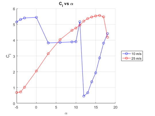
Wait, that’s not right. Never mind the completely erratic data for the lower speed data, the peak Cl value for the high-speed run is just about 4 times higher than one would expect it to be.

It took a bit of digging through the code to find the issue, but basically what had happened was when figuring out the lift on the airfoil, we had figured it out for a chord length of 1. When nondimensionalizing this lift into Cl, we divided by the chord length, which we did not need to do. Given that the chord length is about .25 m, this resulted in Cl values about 4 times higher than they should be.

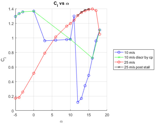
That’s better, as long as we, again, ignore the low speed run. Somewhere along the way, we got some strange pressure data or lift data that severely affects the Cl values we calculate. But still, analyzing one set of usable data can still provide some insight into the accuracy of that data. Two easy ways to do this for a lift curve are looking at the zero-lift α and the stall α. The most noticeable feature of our calculated lift curve is that it does not actually reach Cl=0, which means that unless our method is wrong, we failed to capture the zero lift α. Some preliminary thoughts on how this happened: we decided as a group to test from α=-5 to -3 in order to capture the zero-lift α, but α=-5° was the lower limit for zero lift for lower Reynolds number flow. When we actually tested, we made a quick decision to change the speed of our second run from 15 m/s to 25 m/s.

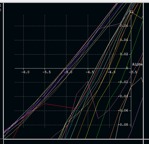
Simulating this new regime in XFLR5 yields a zero-lift α ranging from just above -5° to just below -5° (The group of lines on the left). So, it is likely that speeding the flow up caused our zero-lift α to move outside our test matrix.

The peak Cl is also higher than one would expect. For a higher Re flow, the simulated data shows a peak Cl of about 1.3, not 1.4. Thus, it is possible that for some reason our data has shifted upward on the order of ~.1 Cl.

Referring back to the fixed Cl/α plot, the Cl values for the flow that has separated but not yet reattached is depicted by the black X’s. One thing I mentioned in my last post was wanting to see how the characteristics of the flow changed at equivalent angles of attack for flow that has (a)not yet separated and (b) separated but not yet reattached. The results almost universally showed a Cl greater by ~.05 on the flow that had separated but not reattached. It will take some more thinking to figure why this is, but I initially think that the answer lies in the recirculation occurring in the separated flow, and that this region has a slightly lower pressure than the flow does before it separates, thus imparting a higher lift force. I’m not entirely certain this is the right answer, however.

As I sat, ruminating about the right answer to the question above, as well as trying to figure out our issues with the lift code, I had an interesting (to me) question. How big is the boundary layer on the surface of the Earth? That question is easily answered by the Windows To The Universe website. I thought the website seemed less than reputable at first, but it appears it is written by Earth Science teachers, as well as sponsored through NASA and NOAA. So, we have an answer (50m to 2km, if you don’t want to click the link), but now my question becomes, how would one calculate that? What characteristic length would you use? It’s not like I can Google the equations either. In our classes, we as students are able to simplify things by looking at the closed system only. We assume uniform and simple inlet conditions, and things like that. But on the surface of the Earth, there is no “inlet”. The “wall” that the flow rides on has no beginning and no end. If you wanted to define the starting point for a wall, how would you define the ending point? Sadly, the Earth isn’t flat, so at some point you’re bound to circle around and reach your original starting point. When does the characteristic length “reset”? Suffice it to say, the Earth is a substantially more complex system than a flat plate.

[uniquepandkjf-blog]

process adapt feel tonight swing occur cholesterol realcouncil drawing metal increase bridge get vital opposition

[blogofhistory-blog1]

Death Anniversary..! Satish Dhawan..! 3 January 2002..! #SatishDhawan was an #Indian #Mathematician and #AerospaceEngineer, widely regarded as the "Father of experimental fluid dynamics research" in India..! He was one of the most eminent researchers in the field of #Turbulence and #BoundaryLayers, leading the successful and indigenous development of the Indian space programme..! He succeeded #VikramSarabhai, as #Chairman of the #IndianSpaceResearchOrganisation (#ISRO) in 1972..! https://www.instagram.com/p/BsLS1U2glnWSIbE_Ybnjuzeg2y2TrfW65AoEPM0/?utm_source=ig_tumblr_share&igshid=chq1xtt4exrs

[irispublisherscivilengineering]

Assessment of TC-Dominated Extreme Wind in the Scenario of Climate Change for Wind-Resistant Design of Super-Tall Buildings-Iris Publishers

Authored by  QS Li*

There is a fast development of super-tall buildings during the last decades especially in coastal regions where tropical cyclone (TC) may attack frequently. Owing to their high flexibility, these structures become considerably sensitive to wind, and wind resistant performance has been involved as a critical aspect for the design, construction and maintenance of such civil structures. At TC-prone areas, information of TC wind offers a prerequisite for wind-resistant studies. Previous studies have shown that the greatest uncertainty source for wind-resistant design comes from inaccurate determination of wind information. Therefore, it is of great importance to quantify TC-wind characteristics as accurately as possible. However, wind-related items stipulated in many existing wind load codes/standards are established on the basis of wind measurements for non-TC events in the last century. Meanwhile, these items and many relevant studies account only for the lowest several hundred meters of the atmospheric-boundarylayer (ABL) whose depth has been increasing significantly above ever developing cities. Thus, they can hardly cater for the TCresistant design of super-tall buildings in the future whose heights should exceed one kilometer. Moreover, some detailed features of TC wind should be specially considered for the wind-resistant design of super-tall buildings, although they may be neglected acceptably for the cases of low-to-moderately-high buildings, such as the vertical variation of wind direction (also known as veering/ twisted wind) and air density. Results from field measurements demonstrate that within the ABL, the veering angle of TC wind can accumulate to 20°-45°,and the air density may decrease along height by a factor of ~10% He et al. [1,2]. There is another important issue which has been rarely investigated in the field of wind engineering, i.e., climate-change effect on TC activities and TCdominated extreme wind. It is undoubted that the surface temperature of the earth gets warmer than ever before. 

Read More...Full Text 

For More Articles in Current Trends in Civil & Structural Engineering please click on https://www.irispublishers.com/ctcse

For More Open Access Journals in Iris Publishers please click on https://irispublishers.com/journals.php

To Know indexing list of Iris Publishers please click on

https://medium.com/@irispublishers/what-is-the-indexing-list-of-iris-publishers-4ace353e4eee

To Know more information about Iris Publishers ISSN Number Please click on

https://portal.issn.org/api/search?search[]=MUST=keyproper,keyqualinf,keytitle,notcanc,notinc,notissn,notissnl,unirsrc=irispublishers&search_id=1633309

For Iris publishers Linkedin Please Click on  

https://www.linkedin.com/company/iris-publishers

[priscillanovello]

Surface Layer Study

The objective of this study is the validation of the Boundary Layer (BL) classic theory over Antarctica and study the patterns in the Antarctic region. Another point is to improve the Surface Layer (SL) equations for the Polar Regions in order to have a better representation of the wind fields in the SL of this region. The SL has a turbulent behavior and the major significant variations of momentum, heat and mass occur in the surface layer; hence their great influence on the entire structure of BL. In order to describe and predict the BL, fluid mechanics equations simulate the atmospheric gases dynamics. However, the equations present closure problems. Thereby, solutions were developed based on theories of similarity by Paulson (1970) that, afterwards, had their constants adjusted due to experimental data by Bisunger et. al (1971) and Dyer (1975). This set of solution is known as Businger-Dyer relations. However, the relationship studied do not represent BL in polar regions; Therefore, the models that use the parametrizations based on the theory of similiarity may not represent the global reality, since they are not applicable to the polar regions. In this way, many errors are added to the global climate prediction models that concern economies and policies across the world.

[americanahighways]

Video Premiere: Mark Winters "Boundary Layer"

Video Premiere: Mark Winters "Boundary Layer" #markwinters #boundarylayer #newmusic2022 #buymusic #genefoley

Mark Winters — “Boundary Layer” Americana Highways brings you this premiere of Mark Winters’ song “Boundary Layer,” the title track from his album due to be released on March 11. “Boundary Layer” is Mark Winters on vocals, guitars and bass; Isaias Gil on drums; and Chris Winters on backing vocals.  With footage of ribbons and a stage gig, there’s plenty of visual excitement in the video to…

[iamdahon]

The inner aero nerd in me was like "oooo vortex generators" hahahha #aero #boundarylayer #turbulentflow ✈😁💨👈 (Taken with Instagram at San Francisco International Airport (SFO))