#data.py | Explore Tumblr posts and blogs

sudhirpasala · 5 years ago

Text

Is there an association between age and obesity? ANOVA

Is there an association between age and obesity?

I have selected dataset from my study on food habits across different age groups and Body Mass Index, BMI which is a health indicator related to obesity (Dataset provided at the end, DATCoursera-Data.csv).

The null hypothesis (Ho) of the study is that, "there is no difference in the mean of the quantitative variable, BMI across various age groups as categorical variable". The alternative (Ha) is that there is a difference.

Analysis Of Variance, ANOVA is performed to test the hypothesis. As the statistical test is significant, a post hoc paired comparison using Tukey's HSD is performed to analyze and interpret the result.

DATCoursera-Data.py: import pandas import statsmodels.formula.api as smf from statsmodels.stats.multicomp import pairwise_tukeyhsd

data = pandas.read_csv('DATCoursera-Data.csv')

model1 = smf.ols(formula='BMI~C(AgeCat)', data=data) results1 = model1.fit() print(results1.summary())

m_comp = pairwise_tukeyhsd(endog=data['BMI'], groups=data['AgeCat'], alpha=0.05) print(m_comp)

DATCoursera-Data Console: Python 3.8.3 (default, Jul 2 2020, 17:30:36) [MSC v.1916 64 bit (AMD64)] Type "copyright", "credits" or "license" for more information.

IPython 7.16.1 -- An enhanced Interactive Python.

In [1]: runfile('C:/Users/SUDHIR/.spyder-py3/temp.py', wdir='C:/Users/SUDHIR/.spyder-py3') OLS Regression Results ============================================================================== Dep. Variable: BMI R-squared: 0.125 Model: OLS Adj. R-squared: 0.087 Method: Least Squares F-statistic: 3.297 Date: Fri, 21 Aug 2020 Prob (F-statistic): 0.00807 Time: 10:35:22 Log-Likelihood: -348.53 No. Observations: 121 AIC: 709.1 Df Residuals: 115 BIC: 725.8 Df Model: 5 Covariance Type: nonrobust ================================================================================== coef std err t P>|t| [0.025 0.975] ---------------------------------------------------------------------------------- Intercept 23.8258 0.794 29.990 0.000 22.252 25.399 C(AgeCat)[T.2] 2.3409 1.133 2.066 0.041 0.097 4.585 C(AgeCat)[T.3] 3.8483 1.164 3.305 0.001 1.542 6.155 C(AgeCat)[T.4] 3.5622 1.189 2.996 0.003 1.207 5.917 C(AgeCat)[T.5] 4.3942 2.132 2.061 0.042 0.172 8.617 C(AgeCat)[T.6] 5.8075 2.675 2.171 0.032 0.510 11.105 ============================================================================== Omnibus: 55.069 Durbin-Watson: 1.894 Prob(Omnibus): 0.000 Jarque-Bera (JB): 218.476 Skew: 1.567 Prob(JB): 3.62e-48 Kurtosis: 8.789 Cond. No. 7.51 ==============================================================================

Warnings: [1] Standard Errors assume that the covariance matrix of the errors is correctly specified.

Interpretation: With F-statistic of 3.297 and significant p<0.05 i.e. Prob (F-statistic) of 0.00807, the null hypothesis can be rejected. Hence, there is an association of Age with BMI.

Multiple Comparison of Means - Tukey HSD, FWER=0.05 ==================================================== group1 group2 meandiff p-adj lower upper reject ---------------------------------------------------- 1 2 2.3409 0.3123 -0.9425 5.6242 False 1 3 3.8483 0.0156 0.4735 7.223 True 1 4 3.5622 0.0384 0.116 7.0084 True 1 5 4.3942 0.3149 -1.7842 10.5726 False 1 6 5.8075 0.2592 -1.9441 13.5591 False 2 3 1.5074 0.7666 -1.8934 4.9083 False 2 4 1.2213 0.9 -2.2504 4.693 False 2 5 2.0533 0.9 -4.1394 8.2461 False 2 6 3.4667 0.7611 -4.2963 11.2297 False 3 4 -0.2861 0.9 -3.8444 3.2722 False 3 5 0.5459 0.9 -5.6957 6.7876 False 3 6 1.9593 0.9 -5.8428 9.7614 False 4 5 0.832 0.9 -5.4486 7.1126 False 4 6 2.2453 0.9 -5.5879 10.0786 False 5 6 1.4133 0.9 -7.9492 10.7758 False ----------------------------------------------------

In [2]:

Interpretation: Tukey's HSD multiple comparison of means show significant differences in BMI of C(AgeCat)[T1], 15 to <25 and groups 3 & 4 i.e. age group of C(AgeCat)[T3], 35 to <45 and C(AgeCat)[T4], 45 to <55 respectively.

DATCoursera-Data.csv: Age AgeWise AgeCat Sex BMI Marital status Qualification Profession Non-Veg/Veg. Breakfast Lunch Evening Snacks Dinner Main Course Fruit Intake Milk Tea/Coffee Fruit Juice Buttermilk/Oth Dairy Hot Drinks Beverages Vegetables Leafy Legumes Root/Tuber Cereals Usual Intake of Vegetables Non-Veg. During Lockdown Veg. During Lockdown 15 1 34 2 2 Female 28.3 Married Undergraduate Homebased Yes 2 2 3 2 9 2 0 2 2 2 1 7 0.66 0.66 0.66 0.66 0.66 3.3 9 0 25 2 65 6 6 Male 25.8 Married Doctoral Homebased Yes 2 2 2 2 8 3 0 2 0 2 0 4 1 1 0.66 0.33 1 3.99 5 0 35 3 62 5 5 Male 33.2 Married Post Graduate Homebased Yes 2 2 2 2 8 3 2 0 1 3 0 6 0.66 0.66 0.66 0.66 0.66 3.3 12 0 45 4 27 2 2 Female 28.5 Married Undergraduate Homebased Yes 3 1 3 2 9 3 0 2 3 3 0 8 0.66 0.33 0.66 0.33 1 2.98 3 0 55 5 50 4 4 Female 30.3 Married Undergraduate Homebased Yes 1 1 1 1 4 1 1 1 0 1 0 3 0.66 0.66 0.66 0.66 0.66 3.3 1 0 65 6 42 3 3 Female 25.4 Married Post Graduate Homebased Yes 3 3 3 3 12 3 1 0 1 1 0 3 0.66 0.66 0.66 0.66 0.66 3.3 2 0 75 7 27 2 2 Female 18.4 Married Post Graduate Homebased Yes 2 1 0 2 5 3 2 2 2 2 2 10 1 1 0.66 1 0.66 4.32 12 0 62 5 5 Female 26.1 Married Post Graduate Job No 2 1 0 1 4 3 2 3 2 2 0 9 1 0.66 0.33 0.66 0.33 2.98 0 10 25 2 2 Female 26.7 Single Undergraduate Job No 1 3 0 3 7 3 2 0 1 1 0 4 1 0.66 1 1 1 4.66 0 5 42 3 3 Female 26.8 Married Doctoral Job Yes 3 3 3 3 12 2 0 0 2 0 0 2 1 1 1 1 0.66 4.66 5 0 29 2 2 Female 24.6 Married Post Graduate Job No 2 2 0 2 6 1 0 2 1 1 1 5 1 1 0.66 0.66 0.66 3.98 0 7 65 6 6 Female 35.1 Married Architect Job Yes 0 3 3 3 9 1 1 0 1 3 0 5 1 1 0.66 0.33 0.66 3.65 11 0 49 4 4 Male 24.8 Married Doctoral Job No 0 1 0 1 2 3 0 1 0 1 1 3 0.66 0.66 1 0.33 0.66 3.31 0 5 26 2 2 Male 22.6 Married Post Graduate Job Yes 1 1 1 1 4 1 0 1 1 0 0 2 0.66 0.66 0.33 0.66 0.33 2.64 4 0 31 2 2 Male 23.8 Married Post Graduate Job Yes 1 3 1 3 8 3 2 2 2 2 0 8 1 1 0.66 0.66 1 4.32 9 0 48 4 4 Male 26.2 Married Undergraduate Job No 3 2 1 2 8 2 1 0 2 0 0 3 1 0.66 0.66 1 1 4.32 0 9 48 4 4 Male 26.2 Married Undergraduate Job Yes 0 3 0 3 6 0 0 0 0 0 0 0 0.66 0.33 1 0.33 1 3.32 3 0 45 4 4 Male 26.4 Married Diploma Job Yes 1 2 1 2 6 1 2 2 0 2 0 6 1 1 0.66 1 1 4.66 10 0 48 4 4 Male 34.6 Married Undergraduate Job Yes 3 3 3 3 12 3 3 1 3 3 1 11 0.66 0.33 0.33 0.66 0.66 2.64 15 0 42 3 3 Male 32.5 Married Graduate Job Yes 1 1 3 0 5 1 1 0 1 0 0 2 0.66 1 0.33 0.33 1 3.32 1 0 42 3 3 Male 32.5 Married Graduate Job Yes 0 2 3 2 7 2 1 0 2 2 0 5 1 1 0.66 0.66 1 4.32 12 0 53 4 4 Male 25.8 Married Post Graduate Job Yes 2 2 3 2 9 3 1 1 1 1 0 4 0.66 0.66 0.33 0.66 0.33 2.64 11 0 28 2 2 Male 23.7 Single Undergraduate Job Yes 3 2 3 2 10 3 2 2 0 2 0 6 1 0.66 0.33 1 0.66 3.65 2 0 39 3 3 Male 30.5 Married Doctoral Job Yes 2 2 1 2 7 3 2 2 2 2 0 8 1 0.66 0.66 1 0.66 3.98 0 0 39 3 3 Male 30.5 Married Doctoral Job No 2 3 3 3 11 1 2 1 2 2 3 10 0.66 0.33 0.66 1 0.66 3.31 0 15 49 4 4 Male 30.8 Married Doctoral Job Yes 2 1 0 2 5 1 0 2 0 0 0 2 1 1 0.33 0.33 0.66 3.32 2 0 42 3 3 Male 25 Married Doctoral Job No 1 1 1 1 4 0 1 1 0 1 0 3 0.33 0.33 0.33 0.33 0.33 1.65 0 5 44 3 3 Male 29.4 Married Doctoral Job Yes 2 2 3 2 9 2 2 3 2 2 3 12 1 0.66 0.66 0.66 0.66 3.64 2 0 42 3 3 Male 25 Married Doctoral Job No 2 2 2 2 8 3 2 2 2 0 0 6 0.66 0.66 0.66 0.66 0.66 3.3 0 5 44 3 3 Male 25.1 Married Post Graduate Job Yes 3 2 3 2 10 2 0 1 0 3 1 5 1 0.66 0.66 0.66 1 3.98 0 0 26 2 2 Male 26.8 Single Undergraduate Job Yes 2 2 2 2 8 3 2 2 2 2 2 10 1 0.66 0.66 0.33 0.33 2.98 6 0 43 3 3 Male 24.5 Married Post Graduate Job Yes 2 2 2 2 8 0 0 2 2 3 0 7 0.66 0.66 0.33 0.33 0.66 2.64 10 0 42 3 3 Male 25 Married Doctoral Job Yes 2 2 3 2 9 3 2 3 2 2 0 9 0.66 0.66 0.33 0.33 1 2.98 15 0 42 3 3 Male 25 Married Doctoral Job Yes 2 2 2 1 7 1 1 1 1 2 0 5 1 0.66 0.33 0.66 0.66 3.31 6 0 48 4 4 Male 26.2 Married Undergraduate Job Yes 2 2 2 1 7 1 1 1 1 2 0 5 1 0.66 0.33 0.66 0.66 3.31 6 0 48 4 4 Female 28.3 Married Post Graduate Job No 2 1 0 2 5 0 0 2 0 2 0 4 0.66 0.66 0.66 0.66 1 3.64 0 13 21 1 1 Female 16.2 Single Undergraduate Job No 2 2 1 2 7 2 1 2 3 1 1 8 1 0.33 1 0.66 1 3.99 0 7 41 3 3 Female 26.9 Married Post Graduate Job No 2 2 1 1 6 3 2 1 1 2 0 6 1 0.33 1 1 1 4.33 0 5 58 5 5 Female 23.9 Married Diploma Job Yes 1 2 1 2 6 3 1 2 0 2 0 5 1 1 1 1 1 5 0 0 37 3 3 Female 23.1 Married Post Graduate Job No 1 2 1 2 6 3 3 3 1 3 0 10 1 1 1 1 1 5 0 17 38 3 3 Female 28.3 Married Post Graduate Job Yes 0 3 1 1 5 3 3 0 3 2 1 9 1 0.66 1 1 1 4.66 10 0 50 4 4 Female 33.2 Married Undergraduate Job No 2 2 0 2 6 2 2 3 1 0 2 8 1 1 0.33 0.66 1 3.99 0 7 28 2 2 Female 30.5 Married Post Graduate Job No 1 1 3 1 6 3 0 0 1 3 0 4 1 1 0.66 0.66 0.33 3.65 0 13 45 4 4 Female 24.2 Married Doctoral Job Yes 2 2 1 2 7 2 0 2 2 2 0 6 1 0.66 0.66 0.66 0.33 3.31 12 0 33 2 2 Male 31.2 Married Undergraduate Job Yes 2 2 2 2 8 2 2 2 1 2 0 7 1 0.66 0.66 1 0.33 3.65 9 0 25 2 2 Male 24.2 Single Post Graduate Job Yes 2 2 3 2 9 2 2 0 2 2 0 6 1 1 0.66 0.66 0.66 3.98 9 0 70 6 6 Male 28 Married Doctoral Job No 0 1 0 1 2 0 2 2 3 1 0 8 0.66 0.33 0.66 0.66 0.66 2.97 0 9 52 4 4 Male 22.2 Married Undergraduate Job Yes 2 2 3 1 8 2 2 0 0 2 0 4 1 0.66 0.66 0.33 0.66 3.31 2 0 31 2 2 Male 23 Married Post Graduate Job Yes 3 3 3 3 12 3 3 3 3 3 3 15 0.66 0.66 0.66 0.66 0.66 3.3 13 0 26 2 2 Male 28.4 Single Post Graduate Job Yes 3 2 3 2 10 3 3 3 3 3 0 12 0.33 0.33 1 0.66 1 3.32 11 0 55 5 5 Male 31.2 Married School certificate Job Yes 2 2 2 2 8 3 3 3 3 3 0 12 1 1 1 1 0.33 4.33 7 0 26 2 2 Female 18.8 Single Undergraduate Job Yes 2 2 2 2 8 2 2 3 0 2 0 7 0.66 0.66 0.66 0.66 0.66 3.3 11 0 48 4 4 Female 23.7 Married Post Graduate Job Yes 2 2 2 2 8 3 2 0 0 0 0 2 0.66 0.66 0.33 0.66 0.66 2.97 7 0 50 4 4 Female 24.8 Married Doctoral Job Yes 3 3 3 3 12 1 1 1 0 1 0 3 1 0.66 0.66 0.66 0.66 3.64 6 0 35 3 3 Female 26 Married Post Graduate Job Yes 2 2 2 2 8 2 0 0 2 2 0 4 0.66 1 0.33 1 0.33 3.32 10 0 40 3 3 Male 30.5 Married Doctoral Job Yes 2 3 1 2 8 1 0 0 1 2 0 3 1 0.66 0.33 0.33 0.66 2.98 6 0 45 4 4 Male 30.1 Married Undergraduate Job No 1 2 1 2 6 1 1 1 1 0 0 3 1 0.66 0.66 0.66 1 3.98 0 5 42 3 3 Male 26.8 Married Post Graduate Job Yes 2 2 2 2 8 2 0 3 0 1 0 4 1 0.66 0.33 0.33 1 3.32 13 0 34 2 2 Male 30.1 Married Post Graduate Job Yes 2 2 2 2 8 2 0 3 0 1 0 4 1 0.66 0.33 0.33 1 3.32 13 0 33 2 2 Male 21.5 Married Undergraduate Job Yes 0 1 1 1 3 3 1 1 0 1 0 3 0.66 0.66 1 0.66 0.66 3.64 2 0 27 2 2 Male 42.7 Single Post Graduate Job No 1 3 0 1 5 0 0 0 0 2 0 2 1 0.66 0.66 1 0.66 3.98 0 6 54 4 4 Male 23.9 Married Post Graduate Job Yes 1 2 2 3 8 2 3 0 0 1 0 4 1 1 1 1 1 5 4 0 40 3 3 Male 23.1 Married Post Graduate Job Yes 1 2 0 2 5 1 1 3 1 1 0 6 0.33 0.33 0.66 0.66 1 2.98 11 0 42 3 3 Male 27.1 Married Post Graduate Job Yes 2 1 1 2 6 2 0 2 0 1 0 3 0.66 0.66 0.66 0.66 0.66 3.3 7 0 38 3 3 Male 25.7 Married Doctoral Job Yes 1 1 1 1 4 1 1 1 1 1 0 4 0.66 0.66 0.66 0.66 0.66 3.3 6 0 50 4 4 Male 25.5 Married Post Graduate Job No 1 2 1 2 6 3 0 1 3 2 0 6 1 0.33 0.33 0.66 0.66 2.98 0 14 35 3 3 Male 27.7 Single Doctoral Job Yes 3 1 1 1 6 1 1 0 0 0 0 1 0.33 0.33 0.33 0.66 1 2.65 7 0 29 2 2 Female 22.2 Married Post Graduate Job Yes 1 1 1 1 4 3 1 1 0 1 0 3 0.66 0.66 0.33 0.66 0.66 2.97 14 0 36 3 3 Female 24.9 Married Post Graduate Job Yes 2 2 2 2 8 2 2 2 2 3 2 11 1 1 1 1 1 5 12 0 31 2 2 Male 28.8 Single Undergraduate Job No 2 2 2 2 8 3 2 3 1 1 1 8 0.33 0.33 0.33 0.66 0.66 2.31 0 11 54 4 4 Male 26 Married Doctoral Job Yes 2 2 0 0 4 2 0 2 0 2 0 4 0.66 1 0.66 0.66 0.66 3.64 9 0 25 2 2 Male 20.6 Single Undergraduate Job Yes 1 1 0 1 3 2 0 1 1 1 0 3 0.66 0.66 0.66 0.66 0.33 2.97 2 0 41 3 3 Male 25 Married Undergraduate Job Yes 2 3 3 2 10 2 3 0 1 2 0 6 1 0.66 0.66 1 0.33 3.65 7 0 41 3 3 Male 25 Married Undergraduate Job No 2 0 1 2 5 3 0 1 0 2 0 3 0.66 0.66 0.66 0.66 0.66 3.3 0 5 23 1 1 Male 27.1 Single Undergraduate Job Yes 2 2 3 2 9 1 0 2 0 0 0 2 0.66 0.33 0.33 0.66 0.66 2.64 3 0 33 2 2 Female 27.2 Single Post Graduate Job Yes 2 2 2 2 8 2 0 1 2 2 0 5 1 0.33 0.66 0.66 1 3.65 3 0 30 2 2 Female 22.9 Married Post Graduate Job Yes 1 3 3 1 8 2 2 2 2 2 2 10 1 1 1 1 1 5 12 0 27 2 2 Male 26.9 Single Post Graduate Job No 2 2 0 2 6 0 0 2 0 2 0 4 1 1 0.66 0.66 0.33 3.65 0 11 49 4 4 Male 29.3 Married Undergraduate Job Yes 3 3 3 3 12 3 3 3 3 3 0 12 1 1 0.66 1 1 4.66 6 0 49 4 4 Male 29.3 Married Undergraduate Job Yes 1 1 0 1 3 3 0 1 1 1 0 3 0.66 0.66 0.33 0.66 0.33 2.64 10 0 55 5 5 Male 26.7 Married Undergraduate Job Yes 0 3 0 1 4 3 0 2 0 2 0 4 1 1 1 0.33 1 4.33 4 0 45 4 4 Female 25.8 Married Post Graduate Job No 2 2 0 2 6 3 0 3 0 3 0 6 0.66 0.66 0.66 0.66 0.66 3.3 0 5 23 1 1 Female 21.8 Single Undergraduate Job Yes 3 3 3 3 12 3 2 0 2 3 0 7 1 0.66 0.33 0.33 0.66 2.98 8 0 30 2 2 Male 29.1 Married Undergraduate Job No 2 2 0 2 6 2 0 2 0 1 0 3 1 1 0.66 0.33 1 3.99 0 10 30 2 2 Male 29.1 Married Undergraduate Job No 3 1 0 1 5 1 1 3 2 0 0 6 1 0.33 0.66 1 1 3.99 0 7 41 3 3 Female 49.9 Married Post Graduate Job Yes 2 2 3 3 10 2 2 0 2 3 0 7 1 1 0.66 1 1 4.66 7 0 33 2 2 Female 24.4 Married Post Graduate Job Yes 2 1 3 2 8 1 0 1 1 0 0 2 1 1 1 0.66 1 4.66 7 0 34 2 2 Male 25.7 Single Post Graduate Job Yes 2 1 3 2 8 1 0 1 1 0 0 2 1 1 1 0.66 1 4.66 7 0 23 1 1 Male 24.1 Single Diploma Job Yes 2 2 3 2 9 3 2 2 2 2 0 8 1 1 1 1 1 5 6 0 45 4 4 Female 30.3 Married Post Graduate Job Yes 1 1 1 1 4 3 0 1 1 1 0 3 0.66 0.66 0.66 0.33 0.66 2.97 2 0 26 2 2 Female 24.1 Single Undergraduate Job No 1 1 1 1 4 1 0 2 0 2 0 4 1 1 0.33 1 1 4.33 0 5 47 4 4 Female 31.1 Married Post Graduate Job No 2 2 1 1 6 1 0 2 0 2 0 4 1 0.66 0.66 0.66 0.33 3.31 0 10 50 4 4 Male 25.7 Married Post Graduate Job Yes 2 2 0 2 6 0 2 3 0 0 0 5 0.66 0.66 0.66 0.66 1 3.64 7 0 28 2 2 Male 30.2 Single Post Graduate Job Yes 0 0 0 0 0 2 0 0 0 0 0 0 0.66 0.66 0.66 0.66 0.66 3.3 13 0 23 1 1 Female 25.7 Single School certificate Student Yes 2 3 3 3 11 3 2 3 3 0 0 8 1 0.66 0.66 1 1 4.32 4 0 20 1 1 Female 25.4 Single Undergraduate Student No 2 2 1 1 6 3 2 2 1 1 0 6 0.66 0.66 0.66 0.66 0.66 3.3 0 15 19 1 1 Male 22.6 Single Undergraduate Student Yes 2 2 1 2 7 3 1 0 1 1 0 3 0.66 0.66 0.66 0.33 0.66 2.97 4 0 20 1 1 Male 24.8 Single School certificate Student Yes 0 1 1 1 3 1 0 1 1 1 0 3 0.33 0.33 0.66 0.66 0.66 2.64 5 0 23 1 1 Male 24.8 Single Undergraduate Student Yes 0 0 0 0 0 2 0 0 0 0 0 0 0.66 0.66 0.66 0.66 0.66 3.3 13 0 19 1 1 Male 25.8 Single School certificate Student No 0 0 1 0 1 1 0 1 1 1 1 4 1 1 1 1 1 5 0 5 19 1 1 Male 23.9 Single School certificate Student Yes 1 1 1 1 4 1 0 1 1 1 0 3 0.66 0.33 0.33 0.33 1 2.65 5 0 19 1 1 Female 23.2 Single School certificate Student Yes 1 1 1 1 4 1 0 1 1 1 0 3 0.66 0.33 0.33 0.33 1 2.65 5 0 19 1 1 Female 21.5 Single Undergraduate Student Yes 2 2 2 2 8 2 2 2 1 2 2 9 0.66 1 1 1 0.33 3.99 7 0 20 1 1 Female 24.4 Single School certificate Student Yes 3 3 1 3 10 3 1 0 0 3 0 4 1 0.66 0.33 0.66 1 3.65 3 0 19 1 1 Female 17.7 Single School certificate Student No 1 1 1 1 4 3 3 0 0 0 0 3 0.66 0.66 0.66 0.66 0.66 3.3 0 7 18 1 1 Female 28.5 Single School certificate Student Yes 2 3 2 2 9 2 2 0 0 3 0 5 0.66 0.33 0.33 0.66 1 2.98 7 0 18 1 1 Female 20.9 Single School certificate Student No 2 2 2 2 8 3 2 2 2 2 0 8 0.66 0.33 0.33 0.66 0.66 2.64 0 5 21 1 1 Male 28.3 Single Undergraduate Student No 1 1 1 1 4 2 0 2 0 0 0 2 0.66 0.66 0.66 0.66 0.66 3.3 0 5 21 1 1 Male 15.7 Single Undergraduate Student Yes 2 1 3 2 8 1 0 2 0 2 0 4 0.66 0.66 0.66 0.33 1 3.31 5 0 20 1 1 Male 27.7 Single School certificate Student Yes 2 1 3 2 8 1 0 2 0 2 0 4 0.66 0.66 0.66 0.33 1 3.31 5 0 21 1 1 Male 22.6 Single Diploma Student Yes 0 3 1 2 6 0 0 3 0 3 1 7 0.66 0.33 1 0.66 0.66 3.31 12 0 19 1 1 Male 24.2 Single School certificate Student Yes 3 3 3 3 12 1 2 0 0 0 0 2 1 0.66 0.33 0.66 0.66 3.31 13 0 18 1 1 Male 21.6 Single Undergraduate Student Yes 3 2 0 1 6 1 0 1 1 1 2 5 1 0.33 0.66 1 1 3.99 3 0 19 1 1 Male 17.4 Single School certificate Student No 2 2 2 2 8 3 0 2 3 3 0 8 1 0.66 0.33 0.66 1 3.65 0 13 22 1 1 Male 18.5 Single Undergraduate Student No 1 1 0 1 3 2 0 0 1 0 0 1 0.66 0.66 0.33 0.66 0.66 2.97 0 5 18 1 1 Female 18.6 Single School certificate Student Yes 2 1 0 1 4 3 0 2 3 3 0 8 0.66 1 0.66 0.66 1 3.98 2 0 20 1 1 Male 28.1 Single School certificate Student Yes 3 2 0 1 6 1 0 1 1 1 2 5 1 0.33 0.66 1 1 3.99 3 0 18 1 1 Female 30.5 Single School certificate Student Yes 1 1 1 1 4 1 1 1 1 1 1 5 1 1 1 1 1 5 4 0 19 1 1 Female 33.3 Single Undergraduate Student Yes 0 0 0 0 0 2 0 0 0 0 0 0 0.66 0.66 0.66 0.66 0.66 3.3 13 0 19 1 1 Male 31.6 Single School certificate Student Yes 0 0 0 0 0 2 0 0 0 0 0 0 0.66 0.66 0.66 0.66 0.66 3.3 13 0 20 1 1 Male 22.1 Single Undergraduate Student Yes 2 2 2 1 7 1 1 1 1 2 0 5 1 0.66 0.33 0.66 0.66 3.31 6 0 Note: I have taken the quantitative variable of 'Age' and categorized into six level categorical variables 'AgeCat'. Categorical Variables are as follows, C(AgeCat)[T1], 15 to <25 C(AgeCat)[T2], 25 to <35 C(AgeCat)[T3], 35 to <45 C(AgeCat)[T4], 45 to <55 C(AgeCat)[T5], 55 to <65 C(AgeCat)[T6], Above 65

1 note · View note

freakgeeksworld · 3 years ago

Text

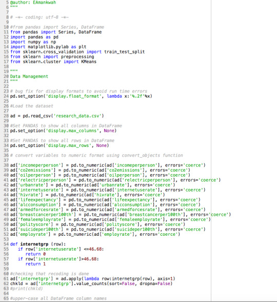
K-meansClustering

The GapMinder data set have been consistently used in all my models and assignments.

A k-means cluster analysis was conducted to identify underlying subgroups of countries based on their similarity of responses on 14 variables that represent characteristics that could have an impact on country demographics/development. Clustering variables included one binary variable measuring whether or not countries internet use rate is high or low, as well as quantitative variables measuring income levels, armed forces strength, level of pollution in terms of co2 emissions, democratic scores, HIV rate, life expectancy rate, oil use rate, and scales measuring alcohol consumption, breast cancer, female employment, suicide, employment, residential electricity and urbanization rates. All clustering variables were standardized to have a mean of 0 and a standard deviation of 1.

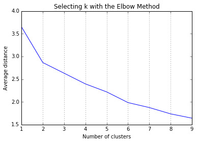
Data were randomly split into a training set that included 70% of the observations (N=38) and a test set that included 30% of the observations (N=17). A series of k-means cluster analyses were conducted on the training data specifying k=1-9 clusters, using Euclidean distance. The variance in the clustering variables that was accounted for by the clusters (r-square) was plotted for each of the nine cluster solutions in an elbow curve to provide guidance for choosing the number of clusters to interpret.

Code:

Results/Interpretation

INCOMEPERPERSON POLITYSCORE CO2EMISSIONS OILPERPERSON HIVRATE \

count 55.00 55.00 55.00 55.00 55.00

mean 12627.14 6.29 17031173042.43 1.08 0.58

std 12545.77 5.89 47219858116.11 0.85 2.38

min 558.06 -10.00 226255333.30 0.03 0.06

25% 2515.64 5.50 1914313500.00 0.44 0.10

50% 6105.28 9.00 4200940333.00 0.81 0.20

75% 25278.09 10.00 11896311167.00 1.56 0.40

max 39972.35 10.00 334000000000.00 4.21 17.80

ALCCONSUMPTION ARMEDFORCESRATE FEMALEEMPLOYRATE \

count 55.00 55.00 55.00

mean 9.57 1.17 46.97

std 5.20 0.82 10.86

min 0.05 0.29 18.20

25% 6.56 0.53 41.90

50% 10.08 0.96 48.00

75% 13.17 1.58 54.45

max 19.15 3.71 68.90

BREASTCANCERPER100TH RELECTRICPERPERSON URBANRATE EMPLOYRATE \

count 55.00 55.00 55.00 55.00

mean 50.26 1461.08 67.49 57.40

std 25.22 1483.93 16.14 7.60

min 16.60 68.12 27.14 41.10

25% 30.55 491.13 60.87 51.85

50% 46.00 830.70 68.46 57.90

75% 74.60 1909.12 77.42 61.90

max 101.10 7432.13 95.64 76.00

INTERNETGRP SUICIDEPER100TH LIFEEXPECTANCY

count 55.00 55.00 55.00

mean 0.49 11.11 75.40

std 0.50 7.04 5.79

min 0.00 1.38 52.80

25% 0.00 5.95 73.05

50% 0.00 10.06 75.63

75% 1.00 13.86 80.49

max 1.00 33.34 83.39

(55, 15)

(38, 14)

/Users/user/anaconda/lib/python3.5/site-packages/sklearn/preprocessing/data.py:167: UserWarning: Numerical issues were encountered when centering the data and might not be solved. Dataset may contain too large values. You may need to prescale your features.

warnings.warn(“Numerical issues were encountered ”

Cluster frequency

0 23

1 15

Name: cluster, dtype: int64

Clustering variable means by cluster

index INCOMEPERPERSON CO2EMISSIONS OILPERPERSON HIVRATE \

cluster

0 81.39 -0.64 -0.21 -0.47 0.18

1 85.07 1.34 0.37 1.18 -0.16

ALCCONSUMPTION ARMEDFORCESRATE FEMALEEMPLOYRATE \

cluster

0 -0.01 0.35 -0.32

1 0.19 -0.60 0.64

RELECTRICPERPERSON BREASTCANCERPER100TH SUICIDEPER100TH URBANRATE \

cluster

0 -0.57 -0.54 0.10 -0.31

1 1.23 1.22 -0.16 0.75

EMPLOYRATE INTERNETGRP LIFEEXPECTANCY

cluster

0 -0.26 -0.55 -0.62

1 0.61 1.02 0.88

OLS Regression Results

=======================================================================Dep. Variable: POLITYSCORE R-squared: 0.115

Model: OLS Adj. R-squared: 0.090

Method: Least Squares F-statistic: 4.678

Date: Mon, 12 Dec 2016 Prob (F-statistic): 0.0373

Time: 13:37:24 Log-Likelihood: -122.22

No. Observations: 38 AIC: 248.4

Df Residuals: 36 BIC: 251.7

Df Model: 1

Covariance Type: nonrobust

========================================================================

coef std err t P>|t| [95.0% Conf. Int.]

———————————————————————————–

Intercept 4.2174 1.293 3.263 0.002 1.596 6.839

C(cluster)[T.1] 4.4493 2.057 2.163 0.037 0.277 8.622

=======================================================================

Omnibus: 16.374 Durbin-Watson: 1.597

Prob(Omnibus): 0.000 Jarque-Bera (JB): 18.322

Skew: -1.554 Prob(JB): 0.000105

Kurtosis: 4.383 Cond. No. 2.44

=======================================================================

Warnings:

[1] Standard Errors assume that the covariance matrix of the errors is correctly specified.

means for POLITYSCORE by cluster

POLITYSCORE

cluster

0 4.22

1 8.67

standard deviations for POLITYSCORE by cluster

POLITYSCORE

cluster

0 6.78

1 5.16

Multiple Comparison of Means - Tukey HSD,FWER=0.05

==========================================

group1 group2 meandiff lower upper reject

——————————————

0 1 4.4493 0.277 8.6215 True

——————————————

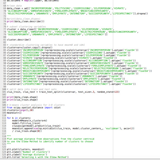
Figure 1. Elbow curve of r-square values for the nine cluster solutions

Summaries

The elbow curve was inconclusive, suggesting that the 2 and 6-cluster solutions might be interpreted. The results below are for an interpretation of the 2-cluster solution.

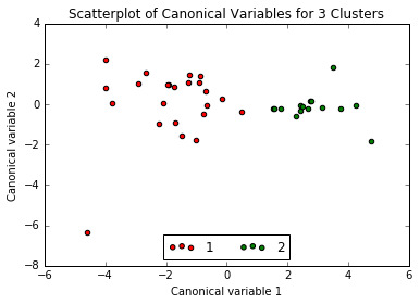
Canonical discriminant analyses was used to reduce the 14 clustering variable down a few variables that accounted for most of the variance in the clustering variables. A scatterplot of the first two canonical variables by cluster (Figure 2 shown below) indicated that the observations in clusters 1 and 2 were sparely packed with relatively low within cluster variance, and did not overlap each other. Observations in cluster 1 were spread out more than clusters 2, showing high within cluster variance. The results of this plot suggest that the best cluster solution may have fewer than 3 clusters, so it will be especially important to also evaluate the cluster solutions with fewer than 3 clusters.

Figure 2. Plot of the first two canonical variables for the clustering variables by cluster.

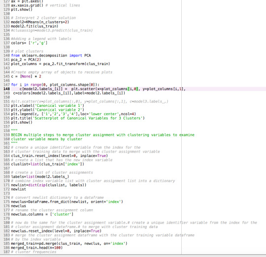
Pattern of Means

The means on the clustering variables showed that, compared to the other clusters, countries in cluster 1 had highest levels on the clustering variables. They had a relatively low likelihood of HIV, armed forces and suicide rates. Countries in cluster 0 had low income levels, oil use rate, co2 emissions, alcohol consumption, female employment rate, residential electricity, breast cancer, urbanization rate, employment rate, low internet use rate and life expectancy rate, and high HIV rate and armed forces. The R square and F statistic value from above show that the clusters differ non-significantly on Polity score.

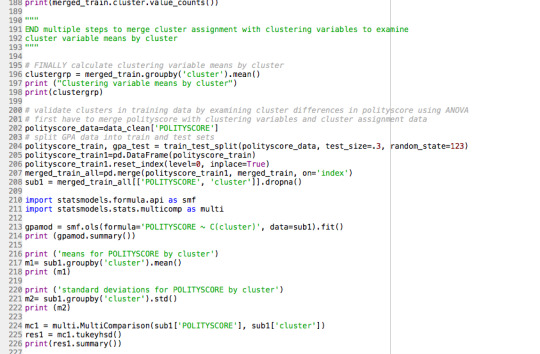
ANOVA - How the clusters differ on Polity Score

In order to externally validate the clusters, an Analysis of Variance (ANOVA) was conducting to test for significant differences between the clusters on polity score (democracy level). A tukey test was used for post hoc comparisons between the clusters. Results indicated significant differences between the clusters on Polity score with p<.05 and F-statistics of 4.68

Countries in cluster 1 have the largest per person polity score (mean = 8.67, s.d = 5.16) while countries in cluster 0 have the lowest polity score globally (mean = 4.22, s.d = 6.78).

0 notes

datab4s3 · 2 years ago

Text

I WAS LOOKING FOR THE TOWN INSIDE ME AND THESE PLAYLISTS SHOWED UP

AND THE BEST PART?

NONE OF THEM HAVE THE TOWN INSIDE ME ON THEM

#guilty gear #guilty gear strive #bridget guilty gear #data.py

37 notes · View notes

holytheoristtastemaker · 5 years ago

Link

Docker Architecture

First, we have to build a docker application with three containers:

ElasticSearch image

Kibana image

Web app image

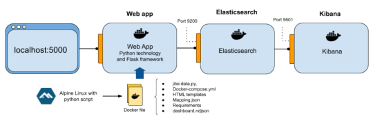
For ElasticSearch and Kibana, we use pre-built images from DockerHub using 7.8.0 version. Web application uses a redis-alpine image.

Note: The reason why using alpine, is because this alternative is smaller and more resource efficient than traditional GNU/Linux distributions (such as Ubuntu)

Required Files And Configuration

You can get the required materials on GitLab. The image below shows the different files you will get by cloning the repo

Docker-compose.yml structure

docker-compose.yml file shows the structure explained in previous section

version: '3' services: web: build: . ports: - 5000:5000 networks: - elastic redis: image: "redis:alpine" es01: image: docker.elastic.co/elasticsearch/elasticsearch:7.8.0 container_name: es01 environment: - node.name=es01 - cluster.name=es-docker-cluster - discovery.type=single-node - bootstrap.memory_lock=true - "ES_JAVA_OPTS=-Xms1024m -Xmx1024m" ulimits: memlock: soft: -1 hard: -1 volumes: - data01:/usr/share/elasticsearch/data ports: - 9200:9200 networks: - elastic kib01: image: docker.elastic.co/kibana/kibana:7.8.0 container_name: kib01 ports: - 5601:5601 environment: ELASTICSEARCH_URL: http://es01:9200 ELASTICSEARCH_HOSTS: http://es01:9200 networks: - elastic volumes: data01: driver: local data02: driver: local data03: driver: local networks: elastic: driver: bridge

Let's take a look at the main tags stated at docker-compose.yml

Ports: configures docker port with host machine port where docker runs. In this case, 5000, 5601 and 9200.

Image: docker image that is downloaded for the required service

Networks: this is named as 'elastic' in order to connect the three services

Environment: configures environment variables essential to operate among services, such as RAM memory parameters. Within Kibana service, it is necessary to define the variables ELASTICSEARCH_URL and ELASTICSEARCH_HOSTS, in order to link it with the Elasticsearch service.

Dockerfile configuration

Dockerfile has the required steps to configure the web application to link with our python script that extract and store the data in an Elasticsearch cluster, that at the same time imports impact_dashboard.ndjson on Kibana for previous visualization.

It runs on alpine distribution to copy the required folders to get the app running. Moreover, and thanks to requirements.txt, you can add all the dependencies that the python script needs.

FROM python:3.7-alpine WORKDIR /code ENV FLASK_APP jitsi-data.py ENV FLASK_RUN_HOST 0.0.0.0 RUN apk add --no-cache git RUN apk add --no-cache tk-dev RUN apk add --no-cache gcc musl-dev linux-headers COPY requirements.txt requirements.txt COPY mapping.json mapping.json COPY templates templates COPY impact_dashboard.ndjson impact_dashboard.ndjson RUN pip install -r requirements.txt EXPOSE 5000 COPY . . CMD ["flask", "run"]

How To Start Containters

In order to start the application (with docker and docker-compose previously installed) open your terminal and execute the following command

$ docker-compose up

This will initiate the different commands stated in dockerfile and download the required docker images. Once that's finished, you can check that Elasticsearch (localhost:9200) and Kibana (localhost:5601) are succesfully running.

Now, it's time to go where python Flask application web app is located, using port 5000

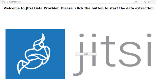
Clicking on start button will initialize data extraction from Jitsi git data (check jitsi-data.py for more details) and will store such data to our ElasticSearch. Finally, it will import impact_dashboard.ndjson to our Kibana, allowing us to interactively play with the data.

Once the process is finished, the browser will show the next message:

Of course, we can see if our Elasticsearch index and Kibana dashboard have successfully being added to our instances:

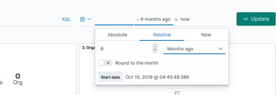
By default the time filter is set to the last 15 minutes. You can use the Time Picker to change the time filter or select a specific time interval or time range in the histogram at the top of the page.

et voilà now you have a cool dashboard up and running to analyze how a pandemic can impact Jitsi software development activity.

Bonus Point: Uploading A Docker Image To Docker Hub

With a Docker Hub account, you can build an image where dockerfile is located. Simply type:

$ docker build -t dockerhubID/DockerHubreponame:imagetag .

Then, upload the image to your Docker Hub repo (you can create the repo using the Docker Hub UI

$ sudo docker push dockerhubID/DockerHubreponame:imagetag

Once the image is uploaded to Docker Hub, any user can use and run the app with the following docker-compose.yml

version: '3' services: web: image: daviddp92/jitsi-data-extraction:1.0.0 ports: - 5000:5000 networks: - elastic es01: image: docker.elastic.co/elasticsearch/elasticsearch:7.8.0 container_name: es01 environment: - node.name=es01 - cluster.name=es-docker-cluster - discovery.type=single-node - bootstrap.memory_lock=true - "ES_JAVA_OPTS=-Xms1024m -Xmx1024m" ulimits: memlock: soft: -1 hard: -1 volumes: - data01:/usr/share/elasticsearch/data ports: - 9200:9200 networks: - elastic kib01: image: docker.elastic.co/kibana/kibana:7.8.0 container_name: kib01 ports: - 5601:5601 environment: ELASTICSEARCH_URL: http://es01:9200 ELASTICSEARCH_HOSTS: http://es01:9200 networks: - elastic volumes: data01: driver: local data02: driver: local data03: driver: local networks: elastic: driver: bridge

Closing thoughts

We have learned how to dockerize a web app with Python technology and Flask framework using docker-compose. We also saw how to use and run the application using Docker Hub images.

0 notes