#i have familiarity w python + sql

[prettyboykatsuki-moved]

are any of u actively working in data science and if u are do u have any advice on how i should approach a technical interview

[anjali11314]

How Can I Get Ready for a Data Science Course in Pune? 

Skilled data scientists are in high demand in today's data-driven environment. A Data Science Course in Pune might be a game-changer for your career, since businesses are depending more and more on data to make choices. To get the most out of your educational experience, you should prepare for your data science course in Pune. We'll go over key preparation measures for your data science course in this blog post so you're ready to go on this thrilling trip. 

Understanding the Basics of Data Science 

It's critical to comprehend the fundamental ideas of data science before delving into the course material. The multidisciplinary area of data science in Pune uses programming, statistical methods, and domain knowledge to draw conclusions from data that are relevant. It will help you if you familiarize yourself with the following ideas: 

Statistics and Probability: A solid grasp of statistical methods and probability theory is crucial for data analysis. Concepts like distributions, hypothesis testing, and regression analysis form the backbone of data science. 

Programming Languages: Python and R are the two most commonly used programming languages in data science. If you're not already familiar with these languages, consider taking a short online course or working through tutorials to build your skills. 

Data Manipulation and Visualization: Learning how to manipulate and visualize data using libraries such as Pandas and Matplotlib (in Python) or ggplot2 (in R) will be immensely helpful. 

By investing time in understanding these foundational concepts, you'll find that the course material is easier to digest, and you can engage more deeply in class discussions. 

Building Your Technical Skills 

Once you’ve familiarized yourself with the basic concepts, the next step is to build your technical skills. A data science course typically involves hands-on projects and coding exercises, so being comfortable with technical tools is essential. Here’s how you can prepare: 

Learn SQL: Data scientists often work with databases to extract and manipulate data. Understanding SQL (Structured Query Language) will help you query databases effectively. 

Familiarize Yourself with Machine Learning: While your course will cover machine learning, having a basic understanding of key algorithms (like linear regression, decision trees, and clustering techniques) can give you an edge. Consider exploring platforms like Coursera or Udacity for introductory machine learning courses. 

Explore Data Science Libraries: Familiarize yourself with popular data science libraries such as Scikit-Learn (for machine learning), TensorFlow (for deep learning), and NumPy (for numerical computations). These libraries are frequently used in data science projects and mastering them will enhance your learning experience. 

By developing these technical skills, you'll be well-prepared to tackle the challenges presented in the course and complete projects with confidence. 

Practical Experience with Data Science Projects 

One of the best ways to get ready for a data science course in Pune is to gain practical experience. Real-world projects allow you to apply your theoretical knowledge, and they can significantly boost your confidence. Here are some steps to consider: 

Kaggle Competitions: Participate in Kaggle competitions to work on real-world data science problems. Kaggle offers datasets and challenges that you can use to hone your skills and build a portfolio. 

Personal Projects: Start a personal data science project based on a topic you're passionate about. Whether it’s analyzing sports statistics, predicting housing prices, or exploring public health data, personal projects can showcase your skills and creativity. 

Contribute to Open Source: Getting involved in open-source projects related to data science can help you learn from experienced developers and gain exposure to collaborative work environments. 

Practical experience will not only deepen your understanding of data science but also provide you with tangible projects to discuss during interviews or networking opportunities. 

Networking and Seeking Guidance 

As you prepare for your data science course, networking can be invaluable. Building relationships with professionals in the field can provide insights and guidance that enhance your learning experience. Here are some ways to connect with others in the data science community: 

Attend Meetups and Workshops: Look for data science meetups, workshops, and seminars in Pune. These events are excellent opportunities to learn from industry experts and meet like-minded individuals. 

Join Online Forums and Communities: Platforms like LinkedIn, Reddit, and specialized data science forums can be great places to connect with others, share resources, and seek advice. 

Find a Mentor: If possible, find a mentor in the field of data science who can provide guidance, share their experiences, and help you navigate your learning journey. 

Networking can open doors to opportunities and provide you with valuable insights that will enhance your education. 

Conclusion 

Preparing for a data science course in Pune is an exciting journey that requires a combination of foundational knowledge, technical skills, practical experience, and networking. By understanding the basics, building your technical abilities, gaining hands-on experience, and connecting with professionals in the field, you’ll be well on your way to success. 

[nexushunter904]

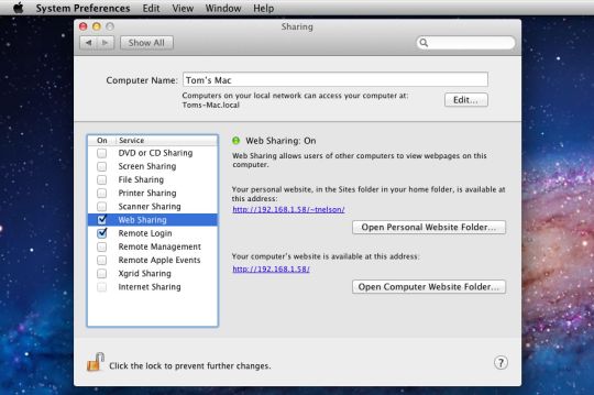
Webserver For Mac

Apache Web Server For Mac

Web Server For Microsoft Edge

Web Server For Mac Os X

Free Web Server For Mac

Web Server For Mac

Are you in need of a web server software for your projects? Looking for something with outstanding performance that suits your prerequisites? A web server is a software program which serves content (HTML documents, images, and other web resources) using the HTTP protocol. It will support both static content and dynamic content. Check these eight top rated web server software and get to know about all its key features here before deciding which would suit your project.

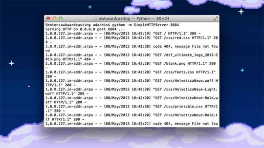
Web server software is a kind of software which is developed to be utilized, controlled and handled on computing server. Web server software gives the exploitation of basic server computing cloud for application with a collection of high-end computing functions and services. This should fire up a webserver that listens on 10.0.1.1:8080 and serves files from the current directory ('.' ) – no PHP, ASP or any of that needed. Any suggestion greatly appreciated. Macos http unix webserver.

Related:

Apache

The Apache HTTP web Server Project is a push to create and keep up an open-source HTTP server for current working frameworks including UNIX and Windows. The objective of this anticipate is to give a safe, effective and extensible server that gives HTTP administrations in a state of harmony with the present HTTP benchmarks.

Virgo Web Server

The Virgo Web Server is the runtime segment of the Virgo Runtime Environment. It is a lightweight, measured, OSGi-based runtime that gives a complete bundled answer for creating, sending, and overseeing venture applications. By utilizing a few best-of-breed advances and enhancing them, the VWS offers a convincing answer for creating and convey endeavor applications.

Abyss Web Server

Abyss Web Server empowers you to have your Web destinations on your PC. It bolsters secure SSL/TLS associations (HTTPS) and in addition an extensive variety of Web innovations. It can likewise run progressed PHP, Perl, Python, ASP, ASP.NET, and Ruby on Rails Web applications which can be sponsored by databases, for example, MySQL, SQLite, MS SQL Server, MS Access, or Oracle.

Cherokee Web Server

All the arrangement is done through Cherokee-Admin, an excellent and effective web interface. Cherokee underpins the most across the board Web innovations: FastCGI, SCGI, PHP, uWSGI, SSI, CGI, LDAP, TLS/SSL, HTTP proxying, video gushing, the content storing, activity forming, and so on. It underpins cross Platform and keeps running on Linux, Mac OS X, and then some more.

Raiden HTTP

RaidenHTTPD is a completely included web server programming for Windows stage. It’s intended for everyone, whether novice or master, who needs to have an intuitive web page running inside minutes. With RaidenHTTPD, everybody can be a web page performer starting now and into the foreseeable future! Having a web page made with RaidenHTTPD, you won’t be surprised to see a great many guests to your web website consistently or considerably more

KF Web Server

KF Web Server is a free HTTP Server that can have a boundless number of websites. Its little size, low framework necessities, and simple organization settle on it the ideal decision for both expert and beginner web designers alike.

Tornado Web Server

Tornado is a Python web structure and offbeat systems administration library, initially created at FriendFeed. By utilizing non-blocking system I/O, Tornado can scale to a huge number of open associations, making it perfect for long surveying, WebSockets, and different applications that require a seemingly perpetual association with every client.

WampServer – Most Popular Software

This is the most mainstream web server amongst all the others. WampServer is a Windows web improvement environment. It permits you to make web applications with Apache2, PHP, and a MySQL database. Nearby, PhpMyAdmin permits you to oversee effortlessly your databases. WampServer is accessible for nothing (under GPML permit) in two particular adaptations that is, 32 and 64 bits.

What is a Web Server?

A Web Server is a PC framework that works by means of HTTP, the system used to disseminate data on the Web. The term can refer to the framework, or to any product particularly that acknowledges and administers the HTTP requests. A web server, in some cases, called an HTTP server or application server is a system that serves content utilizing the HTTP convention. You can also see Log Analyser Software

This substance is often as HTML reports, pictures, and other web assets, however, can incorporate any kind of record. The substance served by the web server can be prior known as a static substance or created on the fly that is alterable content. In a request to be viewed as a web server, an application must actualize the HTTP convention. Applications based on top of web servers. You can also see Proxy Server Software

Therefore, these 8 web servers are very powerful and makes the customer really satisfactory when used in their applications. Try them out and have fun programming!

Related Posts

16 13 likes 31,605 views Last modified Jan 31, 2019 11:25 AM

Here is my definitive guide to getting a local web server running on OS X 10.14 “Mojave”. This is meant to be a development platform so that you can build and test your sites locally, then deploy to an internet server. This User Tip only contains instructions for configuring the Apache server, PHP module, and Perl module. I have another User Tip for installing and configuring MySQL and email servers.

Note: This user tip is specific to macOS 10.14 “Mojave”. Pay attention to your OS version. There have been significant changes since earlier versions of macOS.Another note: These instructions apply to the client versions of OS X, not Server. Server does a few specific tricks really well and is a good choice for those. For things like database, web, and mail services, I have found it easier to just setup the client OS version manually.

Requirements:

Basic understanding of Terminal.app and how to run command-line programs.

Basic understanding of web servers.

Basic usage of vi. You can substitute nano if you want.

Optional: Xcode is required for adding PHP modules.

Lines in bold are what you will have to type in. Lines in bold courier should be typed at the Terminal.Replace <your short user name> with your short user name.

Here goes... Enjoy!

To get started, edit the Apache configuration file as root:

sudo vi /etc/apache2/httpd.conf

Enable PHP by uncommenting line 177, changing:

#LoadModule php7_module libexec/apache2/libphp7.so

to

LoadModule php7_module libexec/apache2/libphp7.so

(If you aren't familiar with vi, go to line 177 by typing '177G' (without the quotes). Then just press 'x' over the '#' character to delete it. Then type ':w!' to save, or just 'ZZ' to save and quit. Don't do that yet though. More changes are still needed.)

If you want to run Perl scripts, you will have to do something similar:

Enable Perl by uncommenting line 178, changing:

#LoadModule perl_module libexec/apache2/mod_perl.so

to

LoadModule perl_module libexec/apache2/mod_perl.so

Enable personal websites by uncommenting the following at line 174:

#LoadModule userdir_module libexec/apache2/mod_userdir.so

to

LoadModule userdir_module libexec/apache2/mod_userdir.so

and do the same at line 511:

#Include /private/etc/apache2/extra/httpd-userdir.conf

to

Apache Web Server For Mac

Include /private/etc/apache2/extra/httpd-userdir.conf

Now save and quit.

Open the file you just enabled above with:

sudo vi /etc/apache2/extra/httpd-userdir.conf

and uncomment the following at line 16:

#Include /private/etc/apache2/users/*.conf

to

Include /private/etc/apache2/users/*.conf

Save and exit.

Lion and later versions no longer create personal web sites by default. If you already had a Sites folder in Snow Leopard, it should still be there. To create one manually, enter the following:

mkdir ~/Sites

echo '<html><body><h1>My site works</h1></body></html>' > ~/Sites/index.html.en

While you are in /etc/apache2, double-check to make sure you have a user config file. It should exist at the path: /etc/apache2/users/<your short user name>.conf.

That file may not exist and if you upgrade from an older version, you may still not have it. It does appear to be created when you create a new user. If that file doesn't exist, you will need to create it with:

sudo vi /etc/apache2/users/<your short user name>.conf

Use the following as the content:

<Directory '/Users/<your short user name>/Sites/'>

AddLanguage en .en

AddHandler perl-script .pl

PerlHandler ModPerl::Registry

Options Indexes MultiViews FollowSymLinks ExecCGI

AllowOverride None

Require host localhost

</Directory>

Now you are ready to turn on Apache itself. But first, do a sanity check. Sometimes copying and pasting from an internet forum can insert invisible, invalid characters into config files. Check your configuration by running the following command in the Terminal:

apachectl configtest

If this command returns 'Syntax OK' then you are ready to go. It may also print a warning saying 'httpd: Could not reliably determine the server's fully qualified domain name'. You could fix this by setting the ServerName directive in /etc/apache2/httpd.conf and adding a matching entry into /etc/hosts. But for a development server, you don't need to do anything. You can just ignore that warning. You can safely ignore other warnings too.

Turn on the Apache httpd service by running the following command in the Terminal:

sudo launchctl load -w /System/Library/LaunchDaemons/org.apache.httpd.plist

In Safari, navigate to your web site with the following address:

http://localhost/

It should say:

It works!

Now try your user home directory:

http://localhost/~<your short user name>

Web Server For Microsoft Edge

It should say:

My site works

Web Server For Mac Os X

Now try PHP. Create a PHP info file with:

echo '<?php echo phpinfo(); ?>' > ~/Sites/info.php

And test it by entering the following into Safari's address bar:

http://localhost/~<your short user name>/info.php

You should see your PHP configuration information.

To test Perl, try something similar. Create a Perl test file with:

echo 'print $ENV(MOD_PERL) . qq(n);' > ~/Sites/info.pl

And test it by entering the following into Safari's address bar:

http://localhost/~<your short user name>/info.pl

Free Web Server For Mac

You should see the string 'mod_perl/2.0.9'.

If you want to setup MySQL, see my User Tip on Installing MySQL.

Web Server For Mac

If you want to add modules to PHP, I suggest the following site. I can't explain it any better.

If you want to make further changes to your Apache system or user config files, you will need to restart the Apache server with:

sudo apachectl graceful

[arcadiadata]

Creating your own data visualization tools

Tableau, PowerBI, and other data visualizations are great at what they do, but it can be painful to do something non-standard. You can often find hacks to get to your desired result..... but sometimes it's just not possible.

Most  analysts and data scientists are skilled in SQL and either Python or R.  But we're not often familiar with Javascript and the various related tools. That’s unfortunate since Javascript can be used to build powerful, interactive visualizations that expand beyond what Tableau and Power BI offer.  

For example, I wanted a visualization to explore data in multiple dimensions. I quickly built this view using Three.JS despite having limited Javascript experience:

(click to try it out)

Although this public view uses a data set based on wine characteristics, there are a couple cool features that I'd like to highlight:

You can click and drag to move the view around.

You can mouse over a datapoint and t information about it will appear in the sidebar

Hit 'w' to see the view pivot automatically as you select different options.

Three.JS plays nicely with VR, so this will be useful for exploring data in VR.

This sort of visualization isn’t relevant in many situations, but it was helpful when I wanted to quickly explore a dataset with high dimensionality.

A couple notes about Javascript:

Javascript struggles with data wrangling (even though dataframe.js is useful in some contexts). I found it more efficient to use Python to do a lot of the initial data work and have Javascript simply ingest the cleaned data. 

Javascript also plays nicely with JSON and other data analysis data formats. 

Although I used Three.js for this tool, it’s useful to know about other options like D3.js, NVD3, etc.  

Github Pages also makes it really easy to host projects.

You can embed webpages within Tableau and thus your Javascript visualization would seem like an integrated part of your Tableau dashboard. 

But just because you can use Javascript to roll your own data visualization, doesn't mean it's always a good investment of your time.

Hit me up on LinkedIn with any questions/feedback...

[alanajacksontx]

Using Python to recover SEO site traffic (Part one)

Helping a client recover from a bad redesign or site migration is probably one of the most critical jobs you can face as an SEO.

The traditional approach of conducting a full forensic SEO audit works well most of the time, but what if there was a way to speed things up? You could potentially save your client a lot of money in opportunity cost.

Last November, I spoke at TechSEO Boost and presented a technique my team and I regularly use to analyze traffic drops. It allows us to pinpoint this painful problem quickly and with surgical precision. As far as I know, there are no tools that currently implement this technique. I coded this solution using Python.

This is the first part of a three-part series. In part two, we will manually group the pages using regular expressions and in part three we will group them automatically using machine learning techniques. Let’s walk over part one and have some fun!

Winners vs losers

Last June we signed up a client that moved from Ecommerce V3 to Shopify and the SEO traffic took a big hit. The owner set up 301 redirects between the old and new sites but made a number of unwise changes like merging a large number of categories and rewriting titles during the move.

When traffic drops, some parts of the site underperform while others don’t. I like to isolate them in order to 1) focus all efforts on the underperforming parts, and 2) learn from the parts that are doing well.

I call this analysis the “Winners vs Losers” analysis. Here, winners are the parts that do well, and losers the ones that do badly.

A visualization of the analysis looks like the chart above. I was able to narrow down the issue to the category pages (Collection pages) and found that the main issue was caused by the site owner merging and eliminating too many categories during the move.

Let’s walk over the steps to put this kind of analysis together in Python.

You can reference my carefully documented Google Colab notebook here.

Getting the data

We want to programmatically compare two separate time frames in Google Analytics (before and after the traffic drop), and we’re going to use the Google Analytics API to do it.

Google Analytics Query Explorer provides the simplest approach to do this in Python.

Head on over to the Google Analytics Query Explorer

Click on the button at the top that says “Click here to Authorize” and follow the steps provided.

Use the dropdown menu to select the website you want to get data from.

Fill in the “metrics” parameter with “ga:newUsers” in order to track new visits.

Complete the “dimensions” parameter with “ga:landingPagePath” in order to get the page URLs.

Fill in the “segment” parameter with “gaid::-5” in order to track organic search visits.

Hit “Run Query” and let it run

Scroll down to the bottom of the page and look for the text box that says “API Query URI.”

Check the box underneath it that says “Include current access_token in the Query URI (will expire in ~60 minutes).”

At the end of the URL in the text box you should now see access_token=string-of-text-here. You will use this string of text in the code snippet below as  the variable called token (make sure to paste it inside the quotes)

Now, scroll back up to where we built the query, and look for the parameter that was filled in for you called “ids.” You will use this in the code snippet below as the variable called “gaid.” Again, it should go inside the quotes.

Run the cell once you’ve filled in the gaid and token variables to instantiate them, and we’re good to go!

First, let’s define placeholder variables to pass to the API

metrics = “,”.join([“ga:users”,”ga:newUsers”])

dimensions = “,”.join([“ga:landingPagePath”, “ga:date”])

segment = “gaid::-5”

# Required, please fill in with your own GA information example: ga:23322342

gaid = “ga:23322342”

# Example: string-of-text-here from step 8.2

token = “”

# Example https://www.example.com or http://example.org

base_site_url = “”

# You can change the start and end dates as you like

start = “2017-06-01”

end = “2018-06-30”

The first function combines the placeholder variables we filled in above with an API URL to get Google Analytics data. We make additional API requests and merge them in case the results exceed the 10,000 limit.

def GAData(gaid, start, end, metrics, dimensions, 

           segment, token, max_results=10000):

  “””Creates a generator that yields GA API data 

     in chunks of size `max_results`”””

  #build uri w/ params

  api_uri = “https://www.googleapis.com/analytics/v3/data/ga?ids={gaid}&”\

             “start-date={start}&end-date={end}&metrics={metrics}&”\

             “dimensions={dimensions}&segment={segment}&access_token={token}&”\

             “max-results={max_results}”

  # insert uri params

  api_uri = api_uri.format(

      gaid=gaid,

      start=start,

      end=end,

      metrics=metrics,

      dimensions=dimensions,

      segment=segment,

      token=token,

      max_results=max_results

  )

  # Using yield to make a generator in an

  # attempt to be memory efficient, since data is downloaded in chunks

  r = requests.get(api_uri)

  data = r.json()

  yield data

  if data.get(“nextLink”, None):

    while data.get(“nextLink”):

      new_uri = data.get(“nextLink”)

      new_uri += “&access_token={token}”.format(token=token)

      r = requests.get(new_uri)

      data = r.json()

      yield data

In the second function, we load the Google Analytics Query Explorer API response into a pandas DataFrame to simplify our analysis.

import pandas as pd

def to_df(gadata):

  “””Takes in a generator from GAData() 

     creates a dataframe from the rows”””

  df = None

  for data in gadata:

    if df is None:

      df = pd.DataFrame(

          data[‘rows’], 

          columns=[x[‘name’] for x in data[‘columnHeaders’]]

      )

    else:

      newdf = pd.DataFrame(

          data[‘rows’], 

          columns=[x[‘name’] for x in data[‘columnHeaders’]]

      )

      df = df.append(newdf)

    print(“Gathered {} rows”.format(len(df)))

  return df

Now, we can call the functions to load the Google Analytics data.

data = GAData(gaid=gaid, metrics=metrics, start=start, 

                end=end, dimensions=dimensions, segment=segment, 

                token=token)

data = to_df(data)

Analyzing the data

Let’s start by just getting a look at the data. We’ll use the .head() method of DataFrames to take a look at the first few rows. Think of this as glancing at only the top few rows of an Excel spreadsheet.

data.head(5)

This displays the first five rows of the data frame.

Most of the data is not in the right format for proper analysis, so let’s perform some data transformations.

First, let’s convert the date to a datetime object and the metrics to numeric values.

data[‘ga:date’] = pd.to_datetime(data[‘ga:date’])

data[‘ga:users’] = pd.to_numeric(data[‘ga:users’])

data[‘ga:newUsers’] = pd.to_numeric(data[‘ga:newUsers’])

Next, we will need the landing page URL, which are relative and include URL parameters in two additional formats: 1) as absolute urls, and 2) as relative paths (without the URL parameters).

from urllib.parse import urlparse, urljoin

data[‘path’] = data[‘ga:landingPagePath’].apply(lambda x: urlparse(x).path)

data[‘url’] = urljoin(base_site_url, data[‘path’])

Now the fun part begins.

The goal of our analysis is to see which pages lost traffic after a particular date–compared to the period before that date–and which gained traffic after that date.

The example date chosen below corresponds to the exact midpoint of our start and end variables used above to gather the data, so that the data both before and after the date is similarly sized.

We begin the analysis by grouping each URL together by their path and adding up the newUsers for each URL. We do this with the built-in pandas method: .groupby(), which takes a column name as an input and groups together each unique value in that column.

The .sum() method then takes the sum of every other column in the data frame within each group.

For more information on these methods please see the Pandas documentation for groupby.

For those who might be familiar with SQL, this is analogous to a GROUP BY clause with a SUM in the select clause

# Change this depending on your needs

MIDPOINT_DATE = “2017-12-15”

before = data[data[‘ga:date’] < pd.to_datetime(MIDPOINT_DATE)]

after = data[data[‘ga:date’] >= pd.to_datetime(MIDPOINT_DATE)]

# Traffic totals before Shopify switch

totals_before = before[[“ga:landingPagePath”, “ga:newUsers”]]\

                .groupby(“ga:landingPagePath”).sum()

totals_before = totals_before.reset_index()\

                .sort_values(“ga:newUsers”, ascending=False)

# Traffic totals after Shopify switch

totals_after = after[[“ga:landingPagePath”, “ga:newUsers”]]\

               .groupby(“ga:landingPagePath”).sum()

totals_after = totals_after.reset_index()\

               .sort_values(“ga:newUsers”, ascending=False)

You can check the totals before and after with this code and double check with the Google Analytics numbers.

print(“Traffic Totals Before: “)

print(“Row count: “, len(totals_before))

print(“Traffic Totals After: “)

print(“Row count: “, len(totals_after))

Next up we merge the two data frames, so that we have a single column corresponding to the URL, and two columns corresponding to the totals before and after the date.

We have different options when merging as illustrated above. Here, we use an “outer” merge, because even if a URL didn’t show up in the “before” period, we still want it to be a part of this merged dataframe. We’ll fill in the blanks with zeros after the merge.

# Comparing pages from before and after the switch

change = totals_after.merge(totals_before, 

                            left_on=”ga:landingPagePath”, 

                            right_on=”ga:landingPagePath”, 

                            suffixes=[“_after”, “_before”], 

                            how=”outer”)

change.fillna(0, inplace=True)

Difference and percentage change

Pandas dataframes make simple calculations on whole columns easy. We can take the difference of two columns and divide two columns and it will perform that operation on every row for us. We will take the difference of the two totals columns, and divide by the “before” column to get the percent change before and after out midpoint date.

Using this percent_change column we can then filter our dataframe to get the winners, the losers and those URLs with no change.

change[‘difference’] = change[‘ga:newUsers_after’] – change[‘ga:newUsers_before’]

change[‘percent_change’] = change[‘difference’] / change[‘ga:newUsers_before’]

winners = change[change[‘percent_change’] > 0]

losers = change[change[‘percent_change’] < 0]

no_change = change[change[‘percent_change’] == 0]

Sanity check

Finally, we do a quick sanity check to make sure that all the traffic from the original data frame is still accounted for after all of our analysis. To do this, we simply take the sum of all traffic for both the original data frame and the two columns of our change dataframe.

# Checking that the total traffic adds up

data[‘ga:newUsers’].sum() == change[[‘ga:newUsers_after’, ‘ga:newUsers_before’]].sum().sum()

It should be True.

Results

Sorting by the difference in our losers data frame, and taking the .head(10), we can see the top 10 losers in our analysis. In other words, these pages lost the most total traffic between the two periods before and after the midpoint date.

losers.sort_values(“difference”).head(10)

You can do the same to review the winners and try to learn from them.

winners.sort_values(“difference”, ascending=False).head(10)

You can export the losing pages to a CSV or Excel using this.

losers.to_csv(“./losing-pages.csv”)

This seems like a lot of work to analyze just one site–and it is!

The magic happens when you reuse this code on new clients and simply need to replace the placeholder variables at the top of the script.

In part two, we will make the output more useful by grouping the losing (and winning) pages by their types to get the chart I included above.

The post Using Python to recover SEO site traffic (Part one) appeared first on Search Engine Watch.

from IM Tips And Tricks https://searchenginewatch.com/2019/02/06/using-python-to-recover-seo-site-traffic-part-one/ from Rising Phoenix SEO https://risingphxseo.tumblr.com/post/182759232745

[kellykperez]

Using Python to recover SEO site traffic (Part one)

Helping a client recover from a bad redesign or site migration is probably one of the most critical jobs you can face as an SEO.

The traditional approach of conducting a full forensic SEO audit works well most of the time, but what if there was a way to speed things up? You could potentially save your client a lot of money in opportunity cost.

Last November, I spoke at TechSEO Boost and presented a technique my team and I regularly use to analyze traffic drops. It allows us to pinpoint this painful problem quickly and with surgical precision. As far as I know, there are no tools that currently implement this technique. I coded this solution using Python.

This is the first part of a three-part series. In part two, we will manually group the pages using regular expressions and in part three we will group them automatically using machine learning techniques. Let’s walk over part one and have some fun!

Winners vs losers

Last June we signed up a client that moved from Ecommerce V3 to Shopify and the SEO traffic took a big hit. The owner set up 301 redirects between the old and new sites but made a number of unwise changes like merging a large number of categories and rewriting titles during the move.

When traffic drops, some parts of the site underperform while others don’t. I like to isolate them in order to 1) focus all efforts on the underperforming parts, and 2) learn from the parts that are doing well.

I call this analysis the “Winners vs Losers” analysis. Here, winners are the parts that do well, and losers the ones that do badly.

A visualization of the analysis looks like the chart above. I was able to narrow down the issue to the category pages (Collection pages) and found that the main issue was caused by the site owner merging and eliminating too many categories during the move.

Let’s walk over the steps to put this kind of analysis together in Python.

You can reference my carefully documented Google Colab notebook here.

Getting the data

We want to programmatically compare two separate time frames in Google Analytics (before and after the traffic drop), and we’re going to use the Google Analytics API to do it.

Google Analytics Query Explorer provides the simplest approach to do this in Python.

Head on over to the Google Analytics Query Explorer

Click on the button at the top that says “Click here to Authorize” and follow the steps provided.

Use the dropdown menu to select the website you want to get data from.

Fill in the “metrics” parameter with “ga:newUsers” in order to track new visits.

Complete the “dimensions” parameter with “ga:landingPagePath” in order to get the page URLs.

Fill in the “segment” parameter with “gaid::-5” in order to track organic search visits.

Hit “Run Query” and let it run

Scroll down to the bottom of the page and look for the text box that says “API Query URI.”

Check the box underneath it that says “Include current access_token in the Query URI (will expire in ~60 minutes).”

At the end of the URL in the text box you should now see access_token=string-of-text-here. You will use this string of text in the code snippet below as  the variable called token (make sure to paste it inside the quotes)

Now, scroll back up to where we built the query, and look for the parameter that was filled in for you called “ids.” You will use this in the code snippet below as the variable called “gaid.” Again, it should go inside the quotes.

Run the cell once you’ve filled in the gaid and token variables to instantiate them, and we’re good to go!

First, let’s define placeholder variables to pass to the API

metrics = “,”.join([“ga:users”,”ga:newUsers”])

dimensions = “,”.join([“ga:landingPagePath”, “ga:date”])

segment = “gaid::-5”

# Required, please fill in with your own GA information example: ga:23322342

gaid = “ga:23322342”

# Example: string-of-text-here from step 8.2

token = “”

# Example https://www.example.com or http://example.org

base_site_url = “”

# You can change the start and end dates as you like

start = “2017-06-01”

end = “2018-06-30”

The first function combines the placeholder variables we filled in above with an API URL to get Google Analytics data. We make additional API requests and merge them in case the results exceed the 10,000 limit.

def GAData(gaid, start, end, metrics, dimensions, 

           segment, token, max_results=10000):

  “””Creates a generator that yields GA API data 

     in chunks of size `max_results`”””

  #build uri w/ params

  api_uri = “https://www.googleapis.com/analytics/v3/data/ga?ids={gaid}&”\

             “start-date={start}&end-date={end}&metrics={metrics}&”\

             “dimensions={dimensions}&segment={segment}&access_token={token}&”\

             “max-results={max_results}”

  # insert uri params

  api_uri = api_uri.format(

      gaid=gaid,

      start=start,

      end=end,

      metrics=metrics,

      dimensions=dimensions,

      segment=segment,

      token=token,

      max_results=max_results

  )

  # Using yield to make a generator in an

  # attempt to be memory efficient, since data is downloaded in chunks

  r = requests.get(api_uri)

  data = r.json()

  yield data

  if data.get(“nextLink”, None):

    while data.get(“nextLink”):

      new_uri = data.get(“nextLink”)

      new_uri += “&access_token={token}”.format(token=token)

      r = requests.get(new_uri)

      data = r.json()

      yield data

In the second function, we load the Google Analytics Query Explorer API response into a pandas DataFrame to simplify our analysis.

import pandas as pd

def to_df(gadata):

  “””Takes in a generator from GAData() 

     creates a dataframe from the rows”””

  df = None

  for data in gadata:

    if df is None:

      df = pd.DataFrame(

          data[‘rows’], 

          columns=[x[‘name’] for x in data[‘columnHeaders’]]

      )

    else:

      newdf = pd.DataFrame(

          data[‘rows’], 

          columns=[x[‘name’] for x in data[‘columnHeaders’]]

      )

      df = df.append(newdf)

    print(“Gathered {} rows”.format(len(df)))

  return df

Now, we can call the functions to load the Google Analytics data.

data = GAData(gaid=gaid, metrics=metrics, start=start, 

                end=end, dimensions=dimensions, segment=segment, 

                token=token)

data = to_df(data)

Analyzing the data

Let’s start by just getting a look at the data. We’ll use the .head() method of DataFrames to take a look at the first few rows. Think of this as glancing at only the top few rows of an Excel spreadsheet.

data.head(5)

This displays the first five rows of the data frame.

Most of the data is not in the right format for proper analysis, so let’s perform some data transformations.

First, let’s convert the date to a datetime object and the metrics to numeric values.

data[‘ga:date’] = pd.to_datetime(data[‘ga:date’])

data[‘ga:users’] = pd.to_numeric(data[‘ga:users’])

data[‘ga:newUsers’] = pd.to_numeric(data[‘ga:newUsers’])

Next, we will need the landing page URL, which are relative and include URL parameters in two additional formats: 1) as absolute urls, and 2) as relative paths (without the URL parameters).

from urllib.parse import urlparse, urljoin

data[‘path’] = data[‘ga:landingPagePath’].apply(lambda x: urlparse(x).path)

data[‘url’] = urljoin(base_site_url, data[‘path’])

Now the fun part begins.

The goal of our analysis is to see which pages lost traffic after a particular date–compared to the period before that date–and which gained traffic after that date.

The example date chosen below corresponds to the exact midpoint of our start and end variables used above to gather the data, so that the data both before and after the date is similarly sized.

We begin the analysis by grouping each URL together by their path and adding up the newUsers for each URL. We do this with the built-in pandas method: .groupby(), which takes a column name as an input and groups together each unique value in that column.

The .sum() method then takes the sum of every other column in the data frame within each group.

For more information on these methods please see the Pandas documentation for groupby.

For those who might be familiar with SQL, this is analogous to a GROUP BY clause with a SUM in the select clause

# Change this depending on your needs

MIDPOINT_DATE = “2017-12-15”

before = data[data[‘ga:date’] < pd.to_datetime(MIDPOINT_DATE)]

after = data[data[‘ga:date’] >= pd.to_datetime(MIDPOINT_DATE)]

# Traffic totals before Shopify switch

totals_before = before[[“ga:landingPagePath”, “ga:newUsers”]]\

                .groupby(“ga:landingPagePath”).sum()

totals_before = totals_before.reset_index()\

                .sort_values(“ga:newUsers”, ascending=False)

# Traffic totals after Shopify switch

totals_after = after[[“ga:landingPagePath”, “ga:newUsers”]]\

               .groupby(“ga:landingPagePath”).sum()

totals_after = totals_after.reset_index()\

               .sort_values(“ga:newUsers”, ascending=False)

You can check the totals before and after with this code and double check with the Google Analytics numbers.

print(“Traffic Totals Before: “)

print(“Row count: “, len(totals_before))

print(“Traffic Totals After: “)

print(“Row count: “, len(totals_after))

Next up we merge the two data frames, so that we have a single column corresponding to the URL, and two columns corresponding to the totals before and after the date.

We have different options when merging as illustrated above. Here, we use an “outer” merge, because even if a URL didn’t show up in the “before” period, we still want it to be a part of this merged dataframe. We’ll fill in the blanks with zeros after the merge.

# Comparing pages from before and after the switch

change = totals_after.merge(totals_before, 

                            left_on=”ga:landingPagePath”, 

                            right_on=”ga:landingPagePath”, 

                            suffixes=[“_after”, “_before”], 

                            how=”outer”)

change.fillna(0, inplace=True)

Difference and percentage change

Pandas dataframes make simple calculations on whole columns easy. We can take the difference of two columns and divide two columns and it will perform that operation on every row for us. We will take the difference of the two totals columns, and divide by the “before” column to get the percent change before and after out midpoint date.

Using this percent_change column we can then filter our dataframe to get the winners, the losers and those URLs with no change.

change[‘difference’] = change[‘ga:newUsers_after’] – change[‘ga:newUsers_before’]

change[‘percent_change’] = change[‘difference’] / change[‘ga:newUsers_before’]

winners = change[change[‘percent_change’] > 0]

losers = change[change[‘percent_change’] < 0]

no_change = change[change[‘percent_change’] == 0]

Sanity check

Finally, we do a quick sanity check to make sure that all the traffic from the original data frame is still accounted for after all of our analysis. To do this, we simply take the sum of all traffic for both the original data frame and the two columns of our change dataframe.

# Checking that the total traffic adds up

data[‘ga:newUsers’].sum() == change[[‘ga:newUsers_after’, ‘ga:newUsers_before’]].sum().sum()

It should be True.

Results

Sorting by the difference in our losers data frame, and taking the .head(10), we can see the top 10 losers in our analysis. In other words, these pages lost the most total traffic between the two periods before and after the midpoint date.

losers.sort_values(“difference”).head(10)

You can do the same to review the winners and try to learn from them.

winners.sort_values(“difference”, ascending=False).head(10)

You can export the losing pages to a CSV or Excel using this.

losers.to_csv(“./losing-pages.csv”)

This seems like a lot of work to analyze just one site–and it is!

The magic happens when you reuse this code on new clients and simply need to replace the placeholder variables at the top of the script.

In part two, we will make the output more useful by grouping the losing (and winning) pages by their types to get the chart I included above.

The post Using Python to recover SEO site traffic (Part one) appeared first on Search Engine Watch.

source https://searchenginewatch.com/2019/02/06/using-python-to-recover-seo-site-traffic-part-one/ from Rising Phoenix SEO http://risingphoenixseo.blogspot.com/2019/02/using-python-to-recover-seo-site.html

[evaaguilaus]

Using Python to recover SEO site traffic (Part one)

Helping a client recover from a bad redesign or site migration is probably one of the most critical jobs you can face as an SEO.

The traditional approach of conducting a full forensic SEO audit works well most of the time, but what if there was a way to speed things up? You could potentially save your client a lot of money in opportunity cost.

Last November, I spoke at TechSEO Boost and presented a technique my team and I regularly use to analyze traffic drops. It allows us to pinpoint this painful problem quickly and with surgical precision. As far as I know, there are no tools that currently implement this technique. I coded this solution using Python.

This is the first part of a three-part series. In part two, we will manually group the pages using regular expressions and in part three we will group them automatically using machine learning techniques. Let’s walk over part one and have some fun!

Winners vs losers

Last June we signed up a client that moved from Ecommerce V3 to Shopify and the SEO traffic took a big hit. The owner set up 301 redirects between the old and new sites but made a number of unwise changes like merging a large number of categories and rewriting titles during the move.

When traffic drops, some parts of the site underperform while others don’t. I like to isolate them in order to 1) focus all efforts on the underperforming parts, and 2) learn from the parts that are doing well.

I call this analysis the “Winners vs Losers” analysis. Here, winners are the parts that do well, and losers the ones that do badly.

A visualization of the analysis looks like the chart above. I was able to narrow down the issue to the category pages (Collection pages) and found that the main issue was caused by the site owner merging and eliminating too many categories during the move.

Let’s walk over the steps to put this kind of analysis together in Python.

You can reference my carefully documented Google Colab notebook here.

Getting the data

We want to programmatically compare two separate time frames in Google Analytics (before and after the traffic drop), and we’re going to use the Google Analytics API to do it.

Google Analytics Query Explorer provides the simplest approach to do this in Python.

Head on over to the Google Analytics Query Explorer

Click on the button at the top that says “Click here to Authorize” and follow the steps provided.

Use the dropdown menu to select the website you want to get data from.

Fill in the “metrics” parameter with “ga:newUsers” in order to track new visits.

Complete the “dimensions” parameter with “ga:landingPagePath” in order to get the page URLs.

Fill in the “segment” parameter with “gaid::-5” in order to track organic search visits.

Hit “Run Query” and let it run

Scroll down to the bottom of the page and look for the text box that says “API Query URI.”

Check the box underneath it that says “Include current access_token in the Query URI (will expire in ~60 minutes).”

At the end of the URL in the text box you should now see access_token=string-of-text-here. You will use this string of text in the code snippet below as  the variable called token (make sure to paste it inside the quotes)

Now, scroll back up to where we built the query, and look for the parameter that was filled in for you called “ids.” You will use this in the code snippet below as the variable called “gaid.” Again, it should go inside the quotes.

Run the cell once you’ve filled in the gaid and token variables to instantiate them, and we’re good to go!

First, let’s define placeholder variables to pass to the API

metrics = “,”.join([“ga:users”,”ga:newUsers”])

dimensions = “,”.join([“ga:landingPagePath”, “ga:date”])

segment = “gaid::-5”

# Required, please fill in with your own GA information example: ga:23322342

gaid = “ga:23322342”

# Example: string-of-text-here from step 8.2

token = “”

# Example https://www.example.com or http://example.org

base_site_url = “”

# You can change the start and end dates as you like

start = “2017-06-01”

end = “2018-06-30”

The first function combines the placeholder variables we filled in above with an API URL to get Google Analytics data. We make additional API requests and merge them in case the results exceed the 10,000 limit.

def GAData(gaid, start, end, metrics, dimensions, 

           segment, token, max_results=10000):

  “””Creates a generator that yields GA API data 

     in chunks of size `max_results`”””

  #build uri w/ params

  api_uri = “https://www.googleapis.com/analytics/v3/data/ga?ids={gaid}&”\

             “start-date={start}&end-date={end}&metrics={metrics}&”\

             “dimensions={dimensions}&segment={segment}&access_token={token}&”\

             “max-results={max_results}”

  # insert uri params

  api_uri = api_uri.format(

      gaid=gaid,

      start=start,

      end=end,

      metrics=metrics,

      dimensions=dimensions,

      segment=segment,

      token=token,

      max_results=max_results

  )

  # Using yield to make a generator in an

  # attempt to be memory efficient, since data is downloaded in chunks

  r = requests.get(api_uri)

  data = r.json()

  yield data

  if data.get(“nextLink”, None):

    while data.get(“nextLink”):

      new_uri = data.get(“nextLink”)

      new_uri += “&access_token={token}”.format(token=token)

      r = requests.get(new_uri)

      data = r.json()

      yield data

In the second function, we load the Google Analytics Query Explorer API response into a pandas DataFrame to simplify our analysis.

import pandas as pd

def to_df(gadata):

  “””Takes in a generator from GAData() 

     creates a dataframe from the rows”””

  df = None

  for data in gadata:

    if df is None:

      df = pd.DataFrame(

          data[‘rows’], 

          columns=[x[‘name’] for x in data[‘columnHeaders’]]

      )

    else:

      newdf = pd.DataFrame(

          data[‘rows’], 

          columns=[x[‘name’] for x in data[‘columnHeaders’]]

      )

      df = df.append(newdf)

    print(“Gathered {} rows”.format(len(df)))

  return df

Now, we can call the functions to load the Google Analytics data.

data = GAData(gaid=gaid, metrics=metrics, start=start, 

                end=end, dimensions=dimensions, segment=segment, 

                token=token)

data = to_df(data)

Analyzing the data

Let’s start by just getting a look at the data. We’ll use the .head() method of DataFrames to take a look at the first few rows. Think of this as glancing at only the top few rows of an Excel spreadsheet.

data.head(5)

This displays the first five rows of the data frame.

Most of the data is not in the right format for proper analysis, so let’s perform some data transformations.

First, let’s convert the date to a datetime object and the metrics to numeric values.

data[‘ga:date’] = pd.to_datetime(data[‘ga:date’])

data[‘ga:users’] = pd.to_numeric(data[‘ga:users’])

data[‘ga:newUsers’] = pd.to_numeric(data[‘ga:newUsers’])

Next, we will need the landing page URL, which are relative and include URL parameters in two additional formats: 1) as absolute urls, and 2) as relative paths (without the URL parameters).

from urllib.parse import urlparse, urljoin

data[‘path’] = data[‘ga:landingPagePath’].apply(lambda x: urlparse(x).path)

data[‘url’] = urljoin(base_site_url, data[‘path’])

Now the fun part begins.

The goal of our analysis is to see which pages lost traffic after a particular date–compared to the period before that date–and which gained traffic after that date.

The example date chosen below corresponds to the exact midpoint of our start and end variables used above to gather the data, so that the data both before and after the date is similarly sized.

We begin the analysis by grouping each URL together by their path and adding up the newUsers for each URL. We do this with the built-in pandas method: .groupby(), which takes a column name as an input and groups together each unique value in that column.

The .sum() method then takes the sum of every other column in the data frame within each group.

For more information on these methods please see the Pandas documentation for groupby.

For those who might be familiar with SQL, this is analogous to a GROUP BY clause with a SUM in the select clause

# Change this depending on your needs

MIDPOINT_DATE = “2017-12-15”

before = data[data[‘ga:date’] < pd.to_datetime(MIDPOINT_DATE)]

after = data[data[‘ga:date’] >= pd.to_datetime(MIDPOINT_DATE)]

# Traffic totals before Shopify switch

totals_before = before[[“ga:landingPagePath”, “ga:newUsers”]]\

                .groupby(“ga:landingPagePath”).sum()

totals_before = totals_before.reset_index()\

                .sort_values(“ga:newUsers”, ascending=False)

# Traffic totals after Shopify switch

totals_after = after[[“ga:landingPagePath”, “ga:newUsers”]]\

               .groupby(“ga:landingPagePath”).sum()

totals_after = totals_after.reset_index()\

               .sort_values(“ga:newUsers”, ascending=False)

You can check the totals before and after with this code and double check with the Google Analytics numbers.

print(“Traffic Totals Before: “)

print(“Row count: “, len(totals_before))

print(“Traffic Totals After: “)

print(“Row count: “, len(totals_after))

Next up we merge the two data frames, so that we have a single column corresponding to the URL, and two columns corresponding to the totals before and after the date.

We have different options when merging as illustrated above. Here, we use an “outer” merge, because even if a URL didn’t show up in the “before” period, we still want it to be a part of this merged dataframe. We’ll fill in the blanks with zeros after the merge.

# Comparing pages from before and after the switch

change = totals_after.merge(totals_before, 

                            left_on=”ga:landingPagePath”, 

                            right_on=”ga:landingPagePath”, 

                            suffixes=[“_after”, “_before”], 

                            how=”outer”)

change.fillna(0, inplace=True)

Difference and percentage change

Pandas dataframes make simple calculations on whole columns easy. We can take the difference of two columns and divide two columns and it will perform that operation on every row for us. We will take the difference of the two totals columns, and divide by the “before” column to get the percent change before and after out midpoint date.

Using this percent_change column we can then filter our dataframe to get the winners, the losers and those URLs with no change.

change[‘difference’] = change[‘ga:newUsers_after’] – change[‘ga:newUsers_before’]

change[‘percent_change’] = change[‘difference’] / change[‘ga:newUsers_before’]

winners = change[change[‘percent_change’] > 0]

losers = change[change[‘percent_change’] < 0]

no_change = change[change[‘percent_change’] == 0]

Sanity check

Finally, we do a quick sanity check to make sure that all the traffic from the original data frame is still accounted for after all of our analysis. To do this, we simply take the sum of all traffic for both the original data frame and the two columns of our change dataframe.

# Checking that the total traffic adds up

data[‘ga:newUsers’].sum() == change[[‘ga:newUsers_after’, ‘ga:newUsers_before’]].sum().sum()

It should be True.

Results

Sorting by the difference in our losers data frame, and taking the .head(10), we can see the top 10 losers in our analysis. In other words, these pages lost the most total traffic between the two periods before and after the midpoint date.

losers.sort_values(“difference”).head(10)

You can do the same to review the winners and try to learn from them.

winners.sort_values(“difference”, ascending=False).head(10)

You can export the losing pages to a CSV or Excel using this.

losers.to_csv(“./losing-pages.csv”)

This seems like a lot of work to analyze just one site–and it is!

The magic happens when you reuse this code on new clients and simply need to replace the placeholder variables at the top of the script.

In part two, we will make the output more useful by grouping the losing (and winning) pages by their types to get the chart I included above.

The post Using Python to recover SEO site traffic (Part one) appeared first on Search Engine Watch.

from Digtal Marketing News https://searchenginewatch.com/2019/02/06/using-python-to-recover-seo-site-traffic-part-one/

[srasamua]

Using Python to recover SEO site traffic (Part one)

Helping a client recover from a bad redesign or site migration is probably one of the most critical jobs you can face as an SEO.

The traditional approach of conducting a full forensic SEO audit works well most of the time, but what if there was a way to speed things up? You could potentially save your client a lot of money in opportunity cost.

Last November, I spoke at TechSEO Boost and presented a technique my team and I regularly use to analyze traffic drops. It allows us to pinpoint this painful problem quickly and with surgical precision. As far as I know, there are no tools that currently implement this technique. I coded this solution using Python.

This is the first part of a three-part series. In part two, we will manually group the pages using regular expressions and in part three we will group them automatically using machine learning techniques. Let’s walk over part one and have some fun!

Winners vs losers

Last June we signed up a client that moved from Ecommerce V3 to Shopify and the SEO traffic took a big hit. The owner set up 301 redirects between the old and new sites but made a number of unwise changes like merging a large number of categories and rewriting titles during the move.

When traffic drops, some parts of the site underperform while others don’t. I like to isolate them in order to 1) focus all efforts on the underperforming parts, and 2) learn from the parts that are doing well.

I call this analysis the “Winners vs Losers” analysis. Here, winners are the parts that do well, and losers the ones that do badly.

A visualization of the analysis looks like the chart above. I was able to narrow down the issue to the category pages (Collection pages) and found that the main issue was caused by the site owner merging and eliminating too many categories during the move.

Let’s walk over the steps to put this kind of analysis together in Python.

You can reference my carefully documented Google Colab notebook here.

Getting the data

We want to programmatically compare two separate time frames in Google Analytics (before and after the traffic drop), and we’re going to use the Google Analytics API to do it.

Google Analytics Query Explorer provides the simplest approach to do this in Python.

Head on over to the Google Analytics Query Explorer

Click on the button at the top that says “Click here to Authorize” and follow the steps provided.

Use the dropdown menu to select the website you want to get data from.

Fill in the “metrics” parameter with “ga:newUsers” in order to track new visits.

Complete the “dimensions” parameter with “ga:landingPagePath” in order to get the page URLs.

Fill in the “segment” parameter with “gaid::-5” in order to track organic search visits.

Hit “Run Query” and let it run

Scroll down to the bottom of the page and look for the text box that says “API Query URI.”

Check the box underneath it that says “Include current access_token in the Query URI (will expire in ~60 minutes).”

At the end of the URL in the text box you should now see access_token=string-of-text-here. You will use this string of text in the code snippet below as  the variable called token (make sure to paste it inside the quotes)

Now, scroll back up to where we built the query, and look for the parameter that was filled in for you called “ids.” You will use this in the code snippet below as the variable called “gaid.” Again, it should go inside the quotes.

Run the cell once you’ve filled in the gaid and token variables to instantiate them, and we’re good to go!

First, let’s define placeholder variables to pass to the API

metrics = “,”.join([“ga:users”,”ga:newUsers”])

dimensions = “,”.join([“ga:landingPagePath”, “ga:date”])

segment = “gaid::-5”

# Required, please fill in with your own GA information example: ga:23322342

gaid = “ga:23322342”

# Example: string-of-text-here from step 8.2

token = “”

# Example https://www.example.com or http://example.org

base_site_url = “”

# You can change the start and end dates as you like

start = “2017-06-01”

end = “2018-06-30”

The first function combines the placeholder variables we filled in above with an API URL to get Google Analytics data. We make additional API requests and merge them in case the results exceed the 10,000 limit.

def GAData(gaid, start, end, metrics, dimensions, 

           segment, token, max_results=10000):

  “””Creates a generator that yields GA API data 

     in chunks of size `max_results`”””

  #build uri w/ params

  api_uri = “https://www.googleapis.com/analytics/v3/data/ga?ids={gaid}&”\

             “start-date={start}&end-date={end}&metrics={metrics}&”\

             “dimensions={dimensions}&segment={segment}&access_token={token}&”\

             “max-results={max_results}”

  # insert uri params

  api_uri = api_uri.format(

      gaid=gaid,

      start=start,

      end=end,

      metrics=metrics,

      dimensions=dimensions,

      segment=segment,

      token=token,

      max_results=max_results

  )

  # Using yield to make a generator in an

  # attempt to be memory efficient, since data is downloaded in chunks

  r = requests.get(api_uri)

  data = r.json()

  yield data

  if data.get(“nextLink”, None):

    while data.get(“nextLink”):

      new_uri = data.get(“nextLink”)

      new_uri += “&access_token={token}”.format(token=token)

      r = requests.get(new_uri)

      data = r.json()

      yield data

In the second function, we load the Google Analytics Query Explorer API response into a pandas DataFrame to simplify our analysis.

import pandas as pd

def to_df(gadata):

  “””Takes in a generator from GAData() 

     creates a dataframe from the rows”””

  df = None

  for data in gadata:

    if df is None:

      df = pd.DataFrame(

          data[‘rows’], 

          columns=[x[‘name’] for x in data[‘columnHeaders’]]

      )

    else:

      newdf = pd.DataFrame(

          data[‘rows’], 

          columns=[x[‘name’] for x in data[‘columnHeaders’]]

      )

      df = df.append(newdf)

    print(“Gathered {} rows”.format(len(df)))

  return df

Now, we can call the functions to load the Google Analytics data.

data = GAData(gaid=gaid, metrics=metrics, start=start, 

                end=end, dimensions=dimensions, segment=segment, 

                token=token)

data = to_df(data)

Analyzing the data

Let’s start by just getting a look at the data. We’ll use the .head() method of DataFrames to take a look at the first few rows. Think of this as glancing at only the top few rows of an Excel spreadsheet.

data.head(5)

This displays the first five rows of the data frame.

Most of the data is not in the right format for proper analysis, so let’s perform some data transformations.

First, let’s convert the date to a datetime object and the metrics to numeric values.

data[‘ga:date’] = pd.to_datetime(data[‘ga:date’])

data[‘ga:users’] = pd.to_numeric(data[‘ga:users’])

data[‘ga:newUsers’] = pd.to_numeric(data[‘ga:newUsers’])

Next, we will need the landing page URL, which are relative and include URL parameters in two additional formats: 1) as absolute urls, and 2) as relative paths (without the URL parameters).

from urllib.parse import urlparse, urljoin

data[‘path’] = data[‘ga:landingPagePath’].apply(lambda x: urlparse(x).path)

data[‘url’] = urljoin(base_site_url, data[‘path’])

Now the fun part begins.

The goal of our analysis is to see which pages lost traffic after a particular date–compared to the period before that date–and which gained traffic after that date.

The example date chosen below corresponds to the exact midpoint of our start and end variables used above to gather the data, so that the data both before and after the date is similarly sized.

We begin the analysis by grouping each URL together by their path and adding up the newUsers for each URL. We do this with the built-in pandas method: .groupby(), which takes a column name as an input and groups together each unique value in that column.

The .sum() method then takes the sum of every other column in the data frame within each group.

For more information on these methods please see the Pandas documentation for groupby.

For those who might be familiar with SQL, this is analogous to a GROUP BY clause with a SUM in the select clause

# Change this depending on your needs

MIDPOINT_DATE = “2017-12-15”

before = data[data[‘ga:date’] < pd.to_datetime(MIDPOINT_DATE)]

after = data[data[‘ga:date’] >= pd.to_datetime(MIDPOINT_DATE)]

# Traffic totals before Shopify switch

totals_before = before[[“ga:landingPagePath”, “ga:newUsers”]]\

                .groupby(“ga:landingPagePath”).sum()

totals_before = totals_before.reset_index()\

                .sort_values(“ga:newUsers”, ascending=False)

# Traffic totals after Shopify switch

totals_after = after[[“ga:landingPagePath”, “ga:newUsers”]]\

               .groupby(“ga:landingPagePath”).sum()

totals_after = totals_after.reset_index()\

               .sort_values(“ga:newUsers”, ascending=False)

You can check the totals before and after with this code and double check with the Google Analytics numbers.

print(“Traffic Totals Before: “)

print(“Row count: “, len(totals_before))

print(“Traffic Totals After: “)

print(“Row count: “, len(totals_after))

Next up we merge the two data frames, so that we have a single column corresponding to the URL, and two columns corresponding to the totals before and after the date.

We have different options when merging as illustrated above. Here, we use an “outer” merge, because even if a URL didn’t show up in the “before” period, we still want it to be a part of this merged dataframe. We’ll fill in the blanks with zeros after the merge.

# Comparing pages from before and after the switch

change = totals_after.merge(totals_before, 

                            left_on=”ga:landingPagePath”, 

                            right_on=”ga:landingPagePath”, 

                            suffixes=[“_after”, “_before”], 

                            how=”outer”)

change.fillna(0, inplace=True)

Difference and percentage change

Pandas dataframes make simple calculations on whole columns easy. We can take the difference of two columns and divide two columns and it will perform that operation on every row for us. We will take the difference of the two totals columns, and divide by the “before” column to get the percent change before and after out midpoint date.

Using this percent_change column we can then filter our dataframe to get the winners, the losers and those URLs with no change.

change[‘difference’] = change[‘ga:newUsers_after’] – change[‘ga:newUsers_before’]

change[‘percent_change’] = change[‘difference’] / change[‘ga:newUsers_before’]

winners = change[change[‘percent_change’] > 0]

losers = change[change[‘percent_change’] < 0]

no_change = change[change[‘percent_change’] == 0]

Sanity check

Finally, we do a quick sanity check to make sure that all the traffic from the original data frame is still accounted for after all of our analysis. To do this, we simply take the sum of all traffic for both the original data frame and the two columns of our change dataframe.

# Checking that the total traffic adds up

data[‘ga:newUsers’].sum() == change[[‘ga:newUsers_after’, ‘ga:newUsers_before’]].sum().sum()

It should be True.

Results

Sorting by the difference in our losers data frame, and taking the .head(10), we can see the top 10 losers in our analysis. In other words, these pages lost the most total traffic between the two periods before and after the midpoint date.

losers.sort_values(“difference”).head(10)

You can do the same to review the winners and try to learn from them.

winners.sort_values(“difference”, ascending=False).head(10)

You can export the losing pages to a CSV or Excel using this.

losers.to_csv(“./losing-pages.csv”)

This seems like a lot of work to analyze just one site–and it is!

The magic happens when you reuse this code on new clients and simply need to replace the placeholder variables at the top of the script.

In part two, we will make the output more useful by grouping the losing (and winning) pages by their types to get the chart I included above.

The post Using Python to recover SEO site traffic (Part one) appeared first on Search Engine Watch.

from Digtal Marketing News https://searchenginewatch.com/2019/02/06/using-python-to-recover-seo-site-traffic-part-one/

[bambiguertinus]

Using Python to recover SEO site traffic (Part one)

Helping a client recover from a bad redesign or site migration is probably one of the most critical jobs you can face as an SEO.

The traditional approach of conducting a full forensic SEO audit works well most of the time, but what if there was a way to speed things up? You could potentially save your client a lot of money in opportunity cost.

Last November, I spoke at TechSEO Boost and presented a technique my team and I regularly use to analyze traffic drops. It allows us to pinpoint this painful problem quickly and with surgical precision. As far as I know, there are no tools that currently implement this technique. I coded this solution using Python.

This is the first part of a three-part series. In part two, we will manually group the pages using regular expressions and in part three we will group them automatically using machine learning techniques. Let’s walk over part one and have some fun!

Winners vs losers

Last June we signed up a client that moved from Ecommerce V3 to Shopify and the SEO traffic took a big hit. The owner set up 301 redirects between the old and new sites but made a number of unwise changes like merging a large number of categories and rewriting titles during the move.

When traffic drops, some parts of the site underperform while others don’t. I like to isolate them in order to 1) focus all efforts on the underperforming parts, and 2) learn from the parts that are doing well.

I call this analysis the “Winners vs Losers” analysis. Here, winners are the parts that do well, and losers the ones that do badly.

A visualization of the analysis looks like the chart above. I was able to narrow down the issue to the category pages (Collection pages) and found that the main issue was caused by the site owner merging and eliminating too many categories during the move.

Let’s walk over the steps to put this kind of analysis together in Python.

You can reference my carefully documented Google Colab notebook here.

Getting the data

We want to programmatically compare two separate time frames in Google Analytics (before and after the traffic drop), and we’re going to use the Google Analytics API to do it.

Google Analytics Query Explorer provides the simplest approach to do this in Python.

Head on over to the Google Analytics Query Explorer

Click on the button at the top that says “Click here to Authorize” and follow the steps provided.

Use the dropdown menu to select the website you want to get data from.

Fill in the “metrics” parameter with “ga:newUsers” in order to track new visits.

Complete the “dimensions” parameter with “ga:landingPagePath” in order to get the page URLs.

Fill in the “segment” parameter with “gaid::-5” in order to track organic search visits.

Hit “Run Query” and let it run

Scroll down to the bottom of the page and look for the text box that says “API Query URI.”

Check the box underneath it that says “Include current access_token in the Query URI (will expire in ~60 minutes).”

At the end of the URL in the text box you should now see access_token=string-of-text-here. You will use this string of text in the code snippet below as  the variable called token (make sure to paste it inside the quotes)

Now, scroll back up to where we built the query, and look for the parameter that was filled in for you called “ids.” You will use this in the code snippet below as the variable called “gaid.” Again, it should go inside the quotes.

Run the cell once you’ve filled in the gaid and token variables to instantiate them, and we’re good to go!

First, let’s define placeholder variables to pass to the API

metrics = “,”.join([“ga:users”,”ga:newUsers”])

dimensions = “,”.join([“ga:landingPagePath”, “ga:date”])

segment = “gaid::-5”

# Required, please fill in with your own GA information example: ga:23322342

gaid = “ga:23322342”

# Example: string-of-text-here from step 8.2

token = “”

# Example https://www.example.com or http://example.org

base_site_url = “”

# You can change the start and end dates as you like

start = “2017-06-01”

end = “2018-06-30”

The first function combines the placeholder variables we filled in above with an API URL to get Google Analytics data. We make additional API requests and merge them in case the results exceed the 10,000 limit.

def GAData(gaid, start, end, metrics, dimensions, 

           segment, token, max_results=10000):

  “””Creates a generator that yields GA API data 

     in chunks of size `max_results`”””

  #build uri w/ params

  api_uri = “https://www.googleapis.com/analytics/v3/data/ga?ids={gaid}&”\

             “start-date={start}&end-date={end}&metrics={metrics}&”\

             “dimensions={dimensions}&segment={segment}&access_token={token}&”\

             “max-results={max_results}”

  # insert uri params

  api_uri = api_uri.format(

      gaid=gaid,

      start=start,

      end=end,

      metrics=metrics,

      dimensions=dimensions,

      segment=segment,

      token=token,

      max_results=max_results

  )

  # Using yield to make a generator in an

  # attempt to be memory efficient, since data is downloaded in chunks

  r = requests.get(api_uri)

  data = r.json()

  yield data

  if data.get(“nextLink”, None):

    while data.get(“nextLink”):

      new_uri = data.get(“nextLink”)

      new_uri += “&access_token={token}”.format(token=token)

      r = requests.get(new_uri)

      data = r.json()

      yield data

In the second function, we load the Google Analytics Query Explorer API response into a pandas DataFrame to simplify our analysis.

import pandas as pd

def to_df(gadata):

  “””Takes in a generator from GAData() 

     creates a dataframe from the rows”””

  df = None

  for data in gadata:

    if df is None:

      df = pd.DataFrame(

          data[‘rows’], 

          columns=[x[‘name’] for x in data[‘columnHeaders’]]

      )

    else:

      newdf = pd.DataFrame(

          data[‘rows’], 

          columns=[x[‘name’] for x in data[‘columnHeaders’]]

      )

      df = df.append(newdf)

    print(“Gathered {} rows”.format(len(df)))

  return df

Now, we can call the functions to load the Google Analytics data.

data = GAData(gaid=gaid, metrics=metrics, start=start, 

                end=end, dimensions=dimensions, segment=segment, 

                token=token)

data = to_df(data)

Analyzing the data

Let’s start by just getting a look at the data. We’ll use the .head() method of DataFrames to take a look at the first few rows. Think of this as glancing at only the top few rows of an Excel spreadsheet.

data.head(5)

This displays the first five rows of the data frame.

Most of the data is not in the right format for proper analysis, so let’s perform some data transformations.

First, let’s convert the date to a datetime object and the metrics to numeric values.

data[‘ga:date’] = pd.to_datetime(data[‘ga:date’])

data[‘ga:users’] = pd.to_numeric(data[‘ga:users’])

data[‘ga:newUsers’] = pd.to_numeric(data[‘ga:newUsers’])

Next, we will need the landing page URL, which are relative and include URL parameters in two additional formats: 1) as absolute urls, and 2) as relative paths (without the URL parameters).

from urllib.parse import urlparse, urljoin

data[‘path’] = data[‘ga:landingPagePath’].apply(lambda x: urlparse(x).path)

data[‘url’] = urljoin(base_site_url, data[‘path’])

Now the fun part begins.

The goal of our analysis is to see which pages lost traffic after a particular date–compared to the period before that date–and which gained traffic after that date.

The example date chosen below corresponds to the exact midpoint of our start and end variables used above to gather the data, so that the data both before and after the date is similarly sized.

We begin the analysis by grouping each URL together by their path and adding up the newUsers for each URL. We do this with the built-in pandas method: .groupby(), which takes a column name as an input and groups together each unique value in that column.

The .sum() method then takes the sum of every other column in the data frame within each group.

For more information on these methods please see the Pandas documentation for groupby.

For those who might be familiar with SQL, this is analogous to a GROUP BY clause with a SUM in the select clause

# Change this depending on your needs

MIDPOINT_DATE = “2017-12-15”

before = data[data[‘ga:date’] < pd.to_datetime(MIDPOINT_DATE)]

after = data[data[‘ga:date’] >= pd.to_datetime(MIDPOINT_DATE)]

# Traffic totals before Shopify switch

totals_before = before[[“ga:landingPagePath”, “ga:newUsers”]]\

                .groupby(“ga:landingPagePath”).sum()

totals_before = totals_before.reset_index()\

                .sort_values(“ga:newUsers”, ascending=False)

# Traffic totals after Shopify switch

totals_after = after[[“ga:landingPagePath”, “ga:newUsers”]]\

               .groupby(“ga:landingPagePath”).sum()

totals_after = totals_after.reset_index()\

               .sort_values(“ga:newUsers”, ascending=False)

You can check the totals before and after with this code and double check with the Google Analytics numbers.

print(“Traffic Totals Before: “)

print(“Row count: “, len(totals_before))

print(“Traffic Totals After: “)

print(“Row count: “, len(totals_after))

Next up we merge the two data frames, so that we have a single column corresponding to the URL, and two columns corresponding to the totals before and after the date.

We have different options when merging as illustrated above. Here, we use an “outer” merge, because even if a URL didn’t show up in the “before” period, we still want it to be a part of this merged dataframe. We’ll fill in the blanks with zeros after the merge.

# Comparing pages from before and after the switch

change = totals_after.merge(totals_before, 

                            left_on=”ga:landingPagePath”, 

                            right_on=”ga:landingPagePath”, 

                            suffixes=[“_after”, “_before”], 

                            how=”outer”)

change.fillna(0, inplace=True)

Difference and percentage change

Pandas dataframes make simple calculations on whole columns easy. We can take the difference of two columns and divide two columns and it will perform that operation on every row for us. We will take the difference of the two totals columns, and divide by the “before” column to get the percent change before and after out midpoint date.

Using this percent_change column we can then filter our dataframe to get the winners, the losers and those URLs with no change.

change[‘difference’] = change[‘ga:newUsers_after’] – change[‘ga:newUsers_before’]

change[‘percent_change’] = change[‘difference’] / change[‘ga:newUsers_before’]

winners = change[change[‘percent_change’] > 0]

losers = change[change[‘percent_change’] < 0]

no_change = change[change[‘percent_change’] == 0]

Sanity check

Finally, we do a quick sanity check to make sure that all the traffic from the original data frame is still accounted for after all of our analysis. To do this, we simply take the sum of all traffic for both the original data frame and the two columns of our change dataframe.

# Checking that the total traffic adds up

data[‘ga:newUsers’].sum() == change[[‘ga:newUsers_after’, ‘ga:newUsers_before’]].sum().sum()

It should be True.

Results

Sorting by the difference in our losers data frame, and taking the .head(10), we can see the top 10 losers in our analysis. In other words, these pages lost the most total traffic between the two periods before and after the midpoint date.

losers.sort_values(“difference”).head(10)

You can do the same to review the winners and try to learn from them.

winners.sort_values(“difference”, ascending=False).head(10)

You can export the losing pages to a CSV or Excel using this.

losers.to_csv(“./losing-pages.csv”)

This seems like a lot of work to analyze just one site–and it is!

The magic happens when you reuse this code on new clients and simply need to replace the placeholder variables at the top of the script.

In part two, we will make the output more useful by grouping the losing (and winning) pages by their types to get the chart I included above.

The post Using Python to recover SEO site traffic (Part one) appeared first on Search Engine Watch.

from Digtal Marketing News https://searchenginewatch.com/2019/02/06/using-python-to-recover-seo-site-traffic-part-one/

[oscarkruegerus]

Using Python to recover SEO site traffic (Part one)

Helping a client recover from a bad redesign or site migration is probably one of the most critical jobs you can face as an SEO.

The traditional approach of conducting a full forensic SEO audit works well most of the time, but what if there was a way to speed things up? You could potentially save your client a lot of money in opportunity cost.

Last November, I spoke at TechSEO Boost and presented a technique my team and I regularly use to analyze traffic drops. It allows us to pinpoint this painful problem quickly and with surgical precision. As far as I know, there are no tools that currently implement this technique. I coded this solution using Python.

This is the first part of a three-part series. In part two, we will manually group the pages using regular expressions and in part three we will group them automatically using machine learning techniques. Let’s walk over part one and have some fun!

Winners vs losers

Last June we signed up a client that moved from Ecommerce V3 to Shopify and the SEO traffic took a big hit. The owner set up 301 redirects between the old and new sites but made a number of unwise changes like merging a large number of categories and rewriting titles during the move.

When traffic drops, some parts of the site underperform while others don’t. I like to isolate them in order to 1) focus all efforts on the underperforming parts, and 2) learn from the parts that are doing well.

I call this analysis the “Winners vs Losers” analysis. Here, winners are the parts that do well, and losers the ones that do badly.

A visualization of the analysis looks like the chart above. I was able to narrow down the issue to the category pages (Collection pages) and found that the main issue was caused by the site owner merging and eliminating too many categories during the move.

Let’s walk over the steps to put this kind of analysis together in Python.

You can reference my carefully documented Google Colab notebook here.

Getting the data

We want to programmatically compare two separate time frames in Google Analytics (before and after the traffic drop), and we’re going to use the Google Analytics API to do it.

Google Analytics Query Explorer provides the simplest approach to do this in Python.

Head on over to the Google Analytics Query Explorer

Click on the button at the top that says “Click here to Authorize” and follow the steps provided.

Use the dropdown menu to select the website you want to get data from.

Fill in the “metrics” parameter with “ga:newUsers” in order to track new visits.

Complete the “dimensions” parameter with “ga:landingPagePath” in order to get the page URLs.

Fill in the “segment” parameter with “gaid::-5” in order to track organic search visits.

Hit “Run Query” and let it run

Scroll down to the bottom of the page and look for the text box that says “API Query URI.”

Check the box underneath it that says “Include current access_token in the Query URI (will expire in ~60 minutes).”

At the end of the URL in the text box you should now see access_token=string-of-text-here. You will use this string of text in the code snippet below as  the variable called token (make sure to paste it inside the quotes)

Now, scroll back up to where we built the query, and look for the parameter that was filled in for you called “ids.” You will use this in the code snippet below as the variable called “gaid.” Again, it should go inside the quotes.

Run the cell once you’ve filled in the gaid and token variables to instantiate them, and we’re good to go!

First, let’s define placeholder variables to pass to the API

metrics = “,”.join([“ga:users”,”ga:newUsers”])

dimensions = “,”.join([“ga:landingPagePath”, “ga:date”])

segment = “gaid::-5”

# Required, please fill in with your own GA information example: ga:23322342

gaid = “ga:23322342”

# Example: string-of-text-here from step 8.2

token = “”

# Example https://www.example.com or http://example.org

base_site_url = “”

# You can change the start and end dates as you like

start = “2017-06-01”

end = “2018-06-30”

The first function combines the placeholder variables we filled in above with an API URL to get Google Analytics data. We make additional API requests and merge them in case the results exceed the 10,000 limit.

def GAData(gaid, start, end, metrics, dimensions, 

           segment, token, max_results=10000):

  “””Creates a generator that yields GA API data 

     in chunks of size `max_results`”””

  #build uri w/ params

  api_uri = “https://www.googleapis.com/analytics/v3/data/ga?ids={gaid}&”\

             “start-date={start}&end-date={end}&metrics={metrics}&”\

             “dimensions={dimensions}&segment={segment}&access_token={token}&”\

             “max-results={max_results}”

  # insert uri params

  api_uri = api_uri.format(

      gaid=gaid,

      start=start,

      end=end,

      metrics=metrics,

      dimensions=dimensions,

      segment=segment,

      token=token,

      max_results=max_results

  )

  # Using yield to make a generator in an

  # attempt to be memory efficient, since data is downloaded in chunks

  r = requests.get(api_uri)

  data = r.json()

  yield data

  if data.get(“nextLink”, None):

    while data.get(“nextLink”):

      new_uri = data.get(“nextLink”)

      new_uri += “&access_token={token}”.format(token=token)

      r = requests.get(new_uri)

      data = r.json()

      yield data

In the second function, we load the Google Analytics Query Explorer API response into a pandas DataFrame to simplify our analysis.

import pandas as pd

def to_df(gadata):

  “””Takes in a generator from GAData() 

     creates a dataframe from the rows”””

  df = None

  for data in gadata:

    if df is None:

      df = pd.DataFrame(

          data[‘rows’], 

          columns=[x[‘name’] for x in data[‘columnHeaders’]]

      )

    else:

      newdf = pd.DataFrame(

          data[‘rows’], 

          columns=[x[‘name’] for x in data[‘columnHeaders’]]

      )

      df = df.append(newdf)

    print(“Gathered {} rows”.format(len(df)))

  return df

Now, we can call the functions to load the Google Analytics data.

data = GAData(gaid=gaid, metrics=metrics, start=start, 

                end=end, dimensions=dimensions, segment=segment, 

                token=token)

data = to_df(data)

Analyzing the data

Let’s start by just getting a look at the data. We’ll use the .head() method of DataFrames to take a look at the first few rows. Think of this as glancing at only the top few rows of an Excel spreadsheet.

data.head(5)

This displays the first five rows of the data frame.

Most of the data is not in the right format for proper analysis, so let’s perform some data transformations.

First, let’s convert the date to a datetime object and the metrics to numeric values.

data[‘ga:date’] = pd.to_datetime(data[‘ga:date’])

data[‘ga:users’] = pd.to_numeric(data[‘ga:users’])

data[‘ga:newUsers’] = pd.to_numeric(data[‘ga:newUsers’])

Next, we will need the landing page URL, which are relative and include URL parameters in two additional formats: 1) as absolute urls, and 2) as relative paths (without the URL parameters).

from urllib.parse import urlparse, urljoin

data[‘path’] = data[‘ga:landingPagePath’].apply(lambda x: urlparse(x).path)

data[‘url’] = urljoin(base_site_url, data[‘path’])

Now the fun part begins.

The goal of our analysis is to see which pages lost traffic after a particular date–compared to the period before that date–and which gained traffic after that date.

The example date chosen below corresponds to the exact midpoint of our start and end variables used above to gather the data, so that the data both before and after the date is similarly sized.

We begin the analysis by grouping each URL together by their path and adding up the newUsers for each URL. We do this with the built-in pandas method: .groupby(), which takes a column name as an input and groups together each unique value in that column.

The .sum() method then takes the sum of every other column in the data frame within each group.

For more information on these methods please see the Pandas documentation for groupby.

For those who might be familiar with SQL, this is analogous to a GROUP BY clause with a SUM in the select clause

# Change this depending on your needs

MIDPOINT_DATE = “2017-12-15”

before = data[data[‘ga:date’] < pd.to_datetime(MIDPOINT_DATE)]

after = data[data[‘ga:date’] >= pd.to_datetime(MIDPOINT_DATE)]

# Traffic totals before Shopify switch

totals_before = before[[“ga:landingPagePath”, “ga:newUsers”]]\

                .groupby(“ga:landingPagePath”).sum()

totals_before = totals_before.reset_index()\

                .sort_values(“ga:newUsers”, ascending=False)

# Traffic totals after Shopify switch

totals_after = after[[“ga:landingPagePath”, “ga:newUsers”]]\

               .groupby(“ga:landingPagePath”).sum()

totals_after = totals_after.reset_index()\

               .sort_values(“ga:newUsers”, ascending=False)

You can check the totals before and after with this code and double check with the Google Analytics numbers.

print(“Traffic Totals Before: “)

print(“Row count: “, len(totals_before))

print(“Traffic Totals After: “)

print(“Row count: “, len(totals_after))

Next up we merge the two data frames, so that we have a single column corresponding to the URL, and two columns corresponding to the totals before and after the date.

We have different options when merging as illustrated above. Here, we use an “outer” merge, because even if a URL didn’t show up in the “before” period, we still want it to be a part of this merged dataframe. We’ll fill in the blanks with zeros after the merge.

# Comparing pages from before and after the switch

change = totals_after.merge(totals_before, 

                            left_on=”ga:landingPagePath”, 

                            right_on=”ga:landingPagePath”, 

                            suffixes=[“_after”, “_before”], 

                            how=”outer”)

change.fillna(0, inplace=True)

Difference and percentage change

Pandas dataframes make simple calculations on whole columns easy. We can take the difference of two columns and divide two columns and it will perform that operation on every row for us. We will take the difference of the two totals columns, and divide by the “before” column to get the percent change before and after out midpoint date.

Using this percent_change column we can then filter our dataframe to get the winners, the losers and those URLs with no change.

change[‘difference’] = change[‘ga:newUsers_after’] – change[‘ga:newUsers_before’]

change[‘percent_change’] = change[‘difference’] / change[‘ga:newUsers_before’]

winners = change[change[‘percent_change’] > 0]

losers = change[change[‘percent_change’] < 0]

no_change = change[change[‘percent_change’] == 0]

Sanity check

Finally, we do a quick sanity check to make sure that all the traffic from the original data frame is still accounted for after all of our analysis. To do this, we simply take the sum of all traffic for both the original data frame and the two columns of our change dataframe.

# Checking that the total traffic adds up

data[‘ga:newUsers’].sum() == change[[‘ga:newUsers_after’, ‘ga:newUsers_before’]].sum().sum()

It should be True.

Results

Sorting by the difference in our losers data frame, and taking the .head(10), we can see the top 10 losers in our analysis. In other words, these pages lost the most total traffic between the two periods before and after the midpoint date.

losers.sort_values(“difference”).head(10)

You can do the same to review the winners and try to learn from them.

winners.sort_values(“difference”, ascending=False).head(10)

You can export the losing pages to a CSV or Excel using this.

losers.to_csv(“./losing-pages.csv”)

This seems like a lot of work to analyze just one site–and it is!

The magic happens when you reuse this code on new clients and simply need to replace the placeholder variables at the top of the script.

In part two, we will make the output more useful by grouping the losing (and winning) pages by their types to get the chart I included above.

The post Using Python to recover SEO site traffic (Part one) appeared first on Search Engine Watch.

from Digtal Marketing News https://searchenginewatch.com/2019/02/06/using-python-to-recover-seo-site-traffic-part-one/

[sheilalmartinia]

Using Python to recover SEO site traffic (Part one)

Helping a client recover from a bad redesign or site migration is probably one of the most critical jobs you can face as an SEO.

The traditional approach of conducting a full forensic SEO audit works well most of the time, but what if there was a way to speed things up? You could potentially save your client a lot of money in opportunity cost.

Last November, I spoke at TechSEO Boost and presented a technique my team and I regularly use to analyze traffic drops. It allows us to pinpoint this painful problem quickly and with surgical precision. As far as I know, there are no tools that currently implement this technique. I coded this solution using Python.

This is the first part of a three-part series. In part two, we will manually group the pages using regular expressions and in part three we will group them automatically using machine learning techniques. Let’s walk over part one and have some fun!

Winners vs losers

Last June we signed up a client that moved from Ecommerce V3 to Shopify and the SEO traffic took a big hit. The owner set up 301 redirects between the old and new sites but made a number of unwise changes like merging a large number of categories and rewriting titles during the move.

When traffic drops, some parts of the site underperform while others don’t. I like to isolate them in order to 1) focus all efforts on the underperforming parts, and 2) learn from the parts that are doing well.

I call this analysis the “Winners vs Losers” analysis. Here, winners are the parts that do well, and losers the ones that do badly.

A visualization of the analysis looks like the chart above. I was able to narrow down the issue to the category pages (Collection pages) and found that the main issue was caused by the site owner merging and eliminating too many categories during the move.

Let’s walk over the steps to put this kind of analysis together in Python.

You can reference my carefully documented Google Colab notebook here.

Getting the data

We want to programmatically compare two separate time frames in Google Analytics (before and after the traffic drop), and we’re going to use the Google Analytics API to do it.

Google Analytics Query Explorer provides the simplest approach to do this in Python.

Head on over to the Google Analytics Query Explorer

Click on the button at the top that says “Click here to Authorize” and follow the steps provided.

Use the dropdown menu to select the website you want to get data from.

Fill in the “metrics” parameter with “ga:newUsers” in order to track new visits.

Complete the “dimensions” parameter with “ga:landingPagePath” in order to get the page URLs.

Fill in the “segment” parameter with “gaid::-5” in order to track organic search visits.

Hit “Run Query” and let it run

Scroll down to the bottom of the page and look for the text box that says “API Query URI.”

Check the box underneath it that says “Include current access_token in the Query URI (will expire in ~60 minutes).”

At the end of the URL in the text box you should now see access_token=string-of-text-here. You will use this string of text in the code snippet below as  the variable called token (make sure to paste it inside the quotes)

Now, scroll back up to where we built the query, and look for the parameter that was filled in for you called “ids.” You will use this in the code snippet below as the variable called “gaid.” Again, it should go inside the quotes.

Run the cell once you’ve filled in the gaid and token variables to instantiate them, and we’re good to go!

First, let’s define placeholder variables to pass to the API

metrics = “,”.join([“ga:users”,”ga:newUsers”])

dimensions = “,”.join([“ga:landingPagePath”, “ga:date”])

segment = “gaid::-5”

# Required, please fill in with your own GA information example: ga:23322342

gaid = “ga:23322342”

# Example: string-of-text-here from step 8.2

token = “”

# Example https://www.example.com or http://example.org

base_site_url = “”

# You can change the start and end dates as you like

start = “2017-06-01”

end = “2018-06-30”

The first function combines the placeholder variables we filled in above with an API URL to get Google Analytics data. We make additional API requests and merge them in case the results exceed the 10,000 limit.

def GAData(gaid, start, end, metrics, dimensions, 

           segment, token, max_results=10000):

  “””Creates a generator that yields GA API data 

     in chunks of size `max_results`”””

  #build uri w/ params

  api_uri = “https://www.googleapis.com/analytics/v3/data/ga?ids={gaid}&”\

             “start-date={start}&end-date={end}&metrics={metrics}&”\

             “dimensions={dimensions}&segment={segment}&access_token={token}&”\

             “max-results={max_results}”

  # insert uri params

  api_uri = api_uri.format(

      gaid=gaid,

      start=start,

      end=end,

      metrics=metrics,

      dimensions=dimensions,

      segment=segment,

      token=token,

      max_results=max_results

  )

  # Using yield to make a generator in an

  # attempt to be memory efficient, since data is downloaded in chunks

  r = requests.get(api_uri)

  data = r.json()

  yield data

  if data.get(“nextLink”, None):

    while data.get(“nextLink”):

      new_uri = data.get(“nextLink”)

      new_uri += “&access_token={token}”.format(token=token)

      r = requests.get(new_uri)

      data = r.json()

      yield data

In the second function, we load the Google Analytics Query Explorer API response into a pandas DataFrame to simplify our analysis.

import pandas as pd

def to_df(gadata):

  “””Takes in a generator from GAData() 

     creates a dataframe from the rows”””

  df = None

  for data in gadata:

    if df is None:

      df = pd.DataFrame(

          data[‘rows’], 

          columns=[x[‘name’] for x in data[‘columnHeaders’]]

      )

    else:

      newdf = pd.DataFrame(

          data[‘rows’], 

          columns=[x[‘name’] for x in data[‘columnHeaders’]]

      )

      df = df.append(newdf)

    print(“Gathered {} rows”.format(len(df)))

  return df

Now, we can call the functions to load the Google Analytics data.

data = GAData(gaid=gaid, metrics=metrics, start=start, 

                end=end, dimensions=dimensions, segment=segment, 

                token=token)

data = to_df(data)

Analyzing the data

Let’s start by just getting a look at the data. We’ll use the .head() method of DataFrames to take a look at the first few rows. Think of this as glancing at only the top few rows of an Excel spreadsheet.

data.head(5)

This displays the first five rows of the data frame.

Most of the data is not in the right format for proper analysis, so let’s perform some data transformations.

First, let’s convert the date to a datetime object and the metrics to numeric values.

data[‘ga:date’] = pd.to_datetime(data[‘ga:date’])

data[‘ga:users’] = pd.to_numeric(data[‘ga:users’])

data[‘ga:newUsers’] = pd.to_numeric(data[‘ga:newUsers’])

Next, we will need the landing page URL, which are relative and include URL parameters in two additional formats: 1) as absolute urls, and 2) as relative paths (without the URL parameters).

from urllib.parse import urlparse, urljoin

data[‘path’] = data[‘ga:landingPagePath’].apply(lambda x: urlparse(x).path)

data[‘url’] = urljoin(base_site_url, data[‘path’])

Now the fun part begins.

The goal of our analysis is to see which pages lost traffic after a particular date–compared to the period before that date–and which gained traffic after that date.

The example date chosen below corresponds to the exact midpoint of our start and end variables used above to gather the data, so that the data both before and after the date is similarly sized.

We begin the analysis by grouping each URL together by their path and adding up the newUsers for each URL. We do this with the built-in pandas method: .groupby(), which takes a column name as an input and groups together each unique value in that column.

The .sum() method then takes the sum of every other column in the data frame within each group.

For more information on these methods please see the Pandas documentation for groupby.

For those who might be familiar with SQL, this is analogous to a GROUP BY clause with a SUM in the select clause

# Change this depending on your needs

MIDPOINT_DATE = “2017-12-15”

before = data[data[‘ga:date’] < pd.to_datetime(MIDPOINT_DATE)]

after = data[data[‘ga:date’] >= pd.to_datetime(MIDPOINT_DATE)]

# Traffic totals before Shopify switch

totals_before = before[[“ga:landingPagePath”, “ga:newUsers”]]\

                .groupby(“ga:landingPagePath”).sum()

totals_before = totals_before.reset_index()\

                .sort_values(“ga:newUsers”, ascending=False)

# Traffic totals after Shopify switch

totals_after = after[[“ga:landingPagePath”, “ga:newUsers”]]\

               .groupby(“ga:landingPagePath”).sum()

totals_after = totals_after.reset_index()\

               .sort_values(“ga:newUsers”, ascending=False)

You can check the totals before and after with this code and double check with the Google Analytics numbers.

print(“Traffic Totals Before: “)

print(“Row count: “, len(totals_before))

print(“Traffic Totals After: “)

print(“Row count: “, len(totals_after))

Next up we merge the two data frames, so that we have a single column corresponding to the URL, and two columns corresponding to the totals before and after the date.

We have different options when merging as illustrated above. Here, we use an “outer” merge, because even if a URL didn’t show up in the “before” period, we still want it to be a part of this merged dataframe. We’ll fill in the blanks with zeros after the merge.

# Comparing pages from before and after the switch

change = totals_after.merge(totals_before, 

                            left_on=”ga:landingPagePath”, 

                            right_on=”ga:landingPagePath”, 

                            suffixes=[“_after”, “_before”], 

                            how=”outer”)

change.fillna(0, inplace=True)

Difference and percentage change

Pandas dataframes make simple calculations on whole columns easy. We can take the difference of two columns and divide two columns and it will perform that operation on every row for us. We will take the difference of the two totals columns, and divide by the “before” column to get the percent change before and after out midpoint date.

Using this percent_change column we can then filter our dataframe to get the winners, the losers and those URLs with no change.

change[‘difference’] = change[‘ga:newUsers_after’] – change[‘ga:newUsers_before’]

change[‘percent_change’] = change[‘difference’] / change[‘ga:newUsers_before’]

winners = change[change[‘percent_change’] > 0]

losers = change[change[‘percent_change’] < 0]

no_change = change[change[‘percent_change��] == 0]

Sanity check

Finally, we do a quick sanity check to make sure that all the traffic from the original data frame is still accounted for after all of our analysis. To do this, we simply take the sum of all traffic for both the original data frame and the two columns of our change dataframe.

# Checking that the total traffic adds up

data[‘ga:newUsers’].sum() == change[[‘ga:newUsers_after’, ‘ga:newUsers_before’]].sum().sum()

It should be True.

Results

Sorting by the difference in our losers data frame, and taking the .head(10), we can see the top 10 losers in our analysis. In other words, these pages lost the most total traffic between the two periods before and after the midpoint date.

losers.sort_values(“difference”).head(10)

You can do the same to review the winners and try to learn from them.

winners.sort_values(“difference”, ascending=False).head(10)

You can export the losing pages to a CSV or Excel using this.

losers.to_csv(“./losing-pages.csv”)

This seems like a lot of work to analyze just one site–and it is!

The magic happens when you reuse this code on new clients and simply need to replace the placeholder variables at the top of the script.

In part two, we will make the output more useful by grouping the losing (and winning) pages by their types to get the chart I included above.

The post Using Python to recover SEO site traffic (Part one) appeared first on Search Engine Watch.

from Search Engine Watch https://searchenginewatch.com/2019/02/06/using-python-to-recover-seo-site-traffic-part-one/