#removeduplicates

[drasmaabbasi]

How To Find And Remove All Duplicate Photos In Windows 10/11 | Delete Duplicate Photos From Laptop

[neveropen]

Python Program For Removing Duplicates From A Sorted Linked List

Write a function that takes a list sorted in non-decreasing order and deletes any duplicate nodes from the list. The list should only be traversed once. For example if the linked list is 11->11->11->21->43->43->60 then removeDuplicates() should convert the list to 11->21->43->60.  Recommended: Please solve it on “PRACTICE” first, before moving on to the solution. Algorithm: Traverse the list from the head (or start) node. While traversing, compare each node with its next node. If the data of the next node is the same as the current node then delete the next node. Before we delete a node, we need to store […]

[techtoolsfree62]

Duplicate Sentence Checker & Remover

📝 Duplicate Sentence Checker & Remover - Clean Up Your Writing! ✨

Tired of repetitive sentences in your text? This Duplicate Sentence Checker & Remover is here to help: ✔️ Detect duplicate sentences instantly ✔️ Highlight duplicates for easy editing ✔️ Remove duplicates with one click

Perfect for writers, students, and professionals who want clean, concise, and impactful writing. Try it now and polish your content like a pro! 🚀

DuplicateSentenceChecker #ContentEditing #WritingTools #SentenceChecker #TextCleaner #RemoveDuplicates #CleanWriting #EditingTips #ContentCreatorTools #Proofreading #WritersLife #ContentPolishing #OnlineTools #ResponsiveDesign #FreeTools

[warner7us-blog]

📌How to count duplicate rows in excel

Check out our updated software Excel Utilities to remove duplicates Rows in excel. It highlights all duplicates rows and then Excel Utilities software removes all duplicates in seconds. For more info: https://bit.ly/2uBf8Yb

[myprogrammingsolver]

CS Lab 3 Remove Duplicates from an ArrayBag Solution

CS Lab 3 Remove Duplicates from an ArrayBag Solution

Goal In this lab you will explore the implementation of the ADT bag using arrays. You will take an existing implementation and create a new method, removeDuplicates, that will guarantee that each item in the bag occurs only once by removing any extra copies. Resources Appendix D: Creating Classes from Other Classes Chapter 1: Bags Chapter 2: Bag Implementations That Use Arrays In javadoc…

[antspinner]

How to remove duplicate values in ms excel 2007

https://youtu.be/Q7RZHmdzdBc

#howtoremoveduplicate #removeduplicates #removeduplicatesvalue #msexcel2007 #removeduplicatesvaluesinexcel #msexcel

[jarviscodinghub]

COSC1047 Lab #7 solved

COSC1047 Lab #7 solved

Part A) Write the following generic method that returns a new ArrayList. The new list contains the non-duplicate elements from the original list. public static ArrayList removeDuplicates(ArrayList originalList) Use the following program to test your method: https://raw.githubusercontent.com/cosc1047w18/course/master/Lab7/labSevenPartA.java Part B) Write the following generic method that returns…

[commercecurve]

Automate Database Reports with Record Macro Function in Excel

How to use Record Macro Function in Excel to Automate Database Reports?

Automation of Database Reports with the Record Macro Function is useful when you export database reports in excel for your everyday reporting purposes. For example, preparing inventory reports or conducting sales analysis and there is a certain set of repeated steps that you must always follow to prepare the report. If you have identified the steps that are repeated all the time, you can be easily automate them to save time.

In this post, I will explain to you how to use the Record Macro Function in Excel to Automate Database Reports.

Practical applications of Automating Database Reports with Record Macro Function.

Example

Suppose you have a sales database report and you would like to automate it so that you can calculate the total units sold by each sales representative.

Step 1: Save your Excel file as Macro Enabled Workbook.

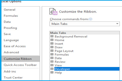
Step 2: Enable Developer Tab in your workbook. Go to File>Options>Customize Ribbon>From Drop Down Select Main Tab>Developer Tab>Add>OK

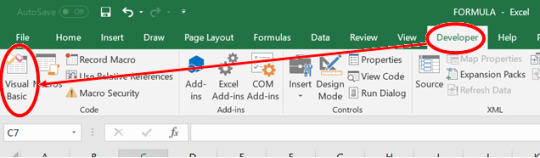
Step 3: From the Developer Tab, click Record Macro and this will prompt you to a Macro Window.

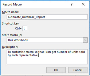
Step 4. (i) Select a name for the Macro. Please note that any spaces in the name should be filled with underscore “_” as it does not allow spaces.

   (ii) Select a short cut key (optional).

   (iii) Option to store the macro in either the same workbook or elsewhere.

   (iv) You can add a description so that you can remember the reason why the macro was created (Recommended).

Step 5: Once you press “OK”, the macro will start recording automatically.

Step 6. You can now proceed to carry out the activity on your database workbook the same way you want it to be automated. In the example above, we will select column C and paste it in Column J. Please make sure not to use any shortcut keys as this can confuse the VBA editor.

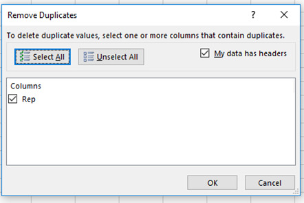
Step 7. Select Column J and go to Data Tab > Remove duplicates. A remove duplicates dialogue box will appear, press OK to get unique representative names.

Step 8: Now Select Cell K1 and name it “Total Units sold”. Below it, type the SUM IF formulae “=SUMIF(C:C,J2,E:E)”. Drag and paste the formulae against all the empty cell. Please make sure not to paste in on the entire column as it will make the worksheet heavy.

Step 9. Go to Developer Tab>Stop Recording. This will stop recording the macro and save it.

Step 10: To view how the VBA has recorded your macro, go to Developer Tab>Visual basic. This will open the VBA editor showing how the formula has been saved. Check for errors and correct them. The formula should look like provided below.

Explanation of the VBA Code

The VBA code shown above is further explained below for the users to understand so that they can customize it themselves if they want the result to be different as per their needs.

   ActiveCell.Offset(0, 2).Columns(“A:A”).EntireColumn.Select

The first layer is simply the Offset function which directs excel to move from one cell to the other based on a specific row and column number. In the beginning, the pre-defined excel cell will be the Cell A1. So, from the Syntax, we are telling excel to move zero rows and two columns forward from the cell A1. Once excel moves to cell C1, we are asking it to select the entire column.

   Selection.Copy

The second layer is instructing excel to copy the selected column.

   ActiveCell.Offset(0, 7).Range(“A1”).Select

In the third layer, we are again using the offset function. Please note, that in this case, the Active Cell has now changed to C1 because of previous selection. After moving seven columns forward from the cell, the new active cell will be the cell J1.

   ActiveSheet.Paste

The fourth layer is instructing excel to paste the copied column on the new active cell.

   ActiveSheet.Range(“J:J”).RemoveDuplicates Columns:=1, Header:=xlYes

The fifth layer is the remove duplicates function. We are simply selecting the entire Column J and removing the duplicate values. The Syntax is also defining that the data for remove duplicates is in one column and it contains a header as well.

  ActiveCell.Offset(0, 1).Range(“A1”).Select

The sixth layer is simply the offset function to select cell K1.

   ActiveCell.FormulaR1C1 = “Total Units Sold”

In seventh layer, we type the header.

   ActiveCell.Offset(1, 0).Range(“A1”).Select

In the eight layer, we are instructing excel to move one row downwards.

   ActiveCell.FormulaR1C1 = “=SUMIF(C[-8],RC[-1],C[-6])”

In the ninth layer, we can see that now the active cell is K2. The code simply enters the SUM IF  formulae where it selects the Column C having the representative names and Column E having the total units sold. The negative numbers represent corresponding column distance from selected cell. Leftward or upward cell movements are represented by a negative sign.

   ActiveCell.Select

   Selection.Copy

   ActiveCell.Offset(1, 0).Range(“A1:A10”).Select

   Selection.PasteSpecial Paste:=xlPasteAll, Operation:=xlNone, SkipBlanks:= _ False, Transpose:=False

The Last part of the VBA code is simply copying the SUM IF formulae to the rest of the representative names to give the result next to each representative name.

Now that you understand how the Record Macro works in Microsoft Excel and stores the VBA Code to automate database reports, you can also customize it as per your needs.

I hope that helps. Please leave a comment below with any questions or suggestions. For more in-depth Excel training, checkout our Ultimate Excel Training Course here. Thank you!

[felord]

SOLVED: Insertion Sort and Generics Insertion Sort and Generics To the GenericArray.java program (provided in the lecture presentation), add a method called removeDuplicates() that removes duplicates from a previously sorted array without disrupting the order.

[photoeditingtips]

Want to find duplicate file on your Mac? Follow this guide to find duplicate file on Mac quickly!

[programmingsolver]

Lab 3 Remove Duplicates from an ArrayBag Solution

Lab 3 Remove Duplicates from an ArrayBag Solution

Goal

In this lab you will explore the implementation of the ADT bag using arrays. You will take an existing implementation and create a new method, removeDuplicates, that will guarantee that each item in the bag occurs only once by removing any extra copies.

Resources

Appendix D: Creating Classes from Other Classes

Chapter 1: Bags

Chapter 2: Bag Implementations That Use Arrays

In javadoc…

[vieclam365vn]

Cách lọc dữ liệu từ nhiều sheet trong excel, bạn đã biết chưa?

1. Tại sao cần phải tiến hành lọc các dữ liệu từ nhiều sheet trong bảng excel? Trong quá trình phân chia công việc hay quản lý các dữ liệu trong một bộ phận, tổ chức, doanh nghiệp hay cả trong quá trình học tập hiện nay, chúng ta thường sẽ sử dụng đến phần mềm excel bởi những tính năng, ứng dụng tiện lợi như là lưu trữ được nhiều thông tin, dữ liệu và có thể phân chia theo từng ô, cột, hàng hay theo các sheet khác nhau để mọi thứ được rõ ràng, tránh nhầm lẫn. Đây cũng chính là công cụ phổ biến nhất được áp dụng trong các công việc văn phòng, đặc biệt là đối với những nhân viên kế toán thì việc sử dụng excel là điều không thể thiếu. Tại sao cần phải tiến hành lọc các dữ liệu từ nhiều sheet trong bảng excel? Tuy nhiên, chắc chắn sẽ có những lúc các thông tin, dữ liệu bạn liệt kê ở các sheet có sự trùng nhau hay nhiều thông tin không cần thiết và khi đó, để tránh xảy ra sự nhầm lẫn, bạn cần phải tiến hành lọc các dữ liệu bị trùng hay gộp những dữ liệu có liên quan đến nhau chung thành một sheet. Và đây cũng chính là thắc mắc của rất nhiều người hiện nay. Và dưới đây sẽ là hướng dẫn chi tiết về cách lọc các dữ liệu từ nhiều sheet trong excel dành cho bạn! 2. Cách lọc dữ liệu từ nhiều sheet trong excel qua cách cơ bản 2.1. Sử dụng hàm Vlookup để lọc dữ liệu từ nhiều sheet trong excel Để có thể lọc dữ liệu từ nhiều sheet trong excel, theo cách cơ bản thường được áp dụng nhất, ví dụ như bạn muốn lọc dữ liệu của 2 sheet thì hãy thực hiện theo các bước sau đây: - Trong sheet 1 bạn sẽ click vào ô đầu tiên để nhập những kết quả trùng, sau đó bạn nhấn vào “tab Formulas” và lựa chọn mục “Insert Function”. - Tiếp đó, trên màn hình sẽ xuất hiện hộp thoại của “Insert Function” và trong đó, bạn sẽ tìm đến “Lookup & Reference” tại phần “Or select a category” bởi thực chất hàm Vlookup thuộc vào nhóm hàm tìm kiếm. Sau đó, bạn kéo xuống phía dưới và sẽ thấy hàm Vlookup rồi nhấn vào OK. - Tiếp sau đó, màn hình sẽ hiển thị phần hộp thoại “Function Arguments” và bạn sẽ thực hiện nhập các vùng dữ liệu cụ thể cho từng yếu tố tại đó. Tại phần “Lookup_value” thì bạn chỉ cần click chuột vào sheet 1 sau đó click tiếp vào ô số C3 (ô đầu tiên trong sheet 1). Như vậy, ô “Lookup_value” sẽ ngay lập tức hiển thị “sheet!C3”. - Bước tiếp theo, tại phần “Table_array” bạn sẽ tiếp tục nhấn vào sheet 2 rồi lựa chọn toàn bộ cùng dữ liệu trùng nhau cần phải tiến hành kiểm tra và trên màn hình sẽ hiển thị “sheet2!C2:E11” (trong đó C2:E11 là ví dụ cho vùng dữ liệu của bạn). Sử dụng hàm Vlookup để lọc dữ liệu từ nhiều sheet trong excel - Một điều bạn cần phải chú ý chính là nếu như muốn thực hiện kiểm tra nhiều vùng dữ liệu hơn thì cần phải thực hiện thao tác cố định các vùng mình lựa chọn thông qua việc nhấp chuột vào chính giữa hoặc cũng có thể là cuối ô C2 rồi nhấn F4 để cố định. Tương tự như vậy thì bạn cũng thực hiện với E11 để cố định vùng dữ liệu. Khi đó, tại “Table_array” sẽ hiển thị “sheet2!$C$2:$E$11”. - Sau khi đã hoàn thành các thao tác trên, bạn sẽ thực hiện nhập 1 vị trí cụ thể mà bạn muốn lưu giữ liệu sau khi lọc tại phần “Col_index_num”. Ví dụ nếu như bạn muốn lưu ở cột đầu tiên thì sẽ nhập số 1. Tiếp đó, tại “Range_lookup” bạn sẽ nhập số 0 để hoàn tất quá trình lọc một cách chính xác nhất rồi nhấp vào OK. - Bước tiếp theo chính là kiểm tra các dữ liệu đã lọc được hiển thị trên màn hình rồi thực hiện thao tác kéo dữ liệu từ ô đầu tiên đi xuống những ô còn lại và những ô không có dữ liệu thì sẽ hiển thị lỗi là #N/A. - Như vậy, cuối cùng bạn sẽ thu được công thức Vlookup để có thể lọc dữ liệu như sau: =VLOOKUP(sheet1!C3,sheet2!$C$2:$E$11,1,0), trong đó cụ thể là: + Sheet1!C3 chính là ô số 3 của cột C trong sheet 1 mà bạn cần phải kiểm tra dữ liệu bị trùng và cần lọc bỏ hay gộp lại. + Sheet2!$C$2:$E$11 chính là vùng dữ liệu mà bạn cần phải kiểm tra để xem có trùng với sheet 2 hay không. - 1 chính là số cột mà bạn muốn kết quả trả về để lưu trữ sau khi đã kiểm tra. - 0 chính là kiểm mà bạn tìm kiếm một cách chính xác nhất hàm Vlookup. 2.2. Sử dụng hàm Vlook kết hợp hàm If, ISNA để lọc dữ liệu từ nhiều sheet trong excel Sau khi đã sử dụng hàm Vlookup để thu được công thức cũng như kiểm tra được các dữ liệu trùng thì trong những ô không trùng sẽ hiển thị các lỗi có ký hiệu là #N/A và khi đó bạn cần kết hợp với hàm ISNA để có thể kiểm tra lại một cách chính xác. Nếu như các dữ liệu hiển thị là #N/A thì hàm ISNA sẽ đưa ra kết quả là TRUE, còn nếu không đúng thì sẽ hiển thị FALSE. Còn đối với hàm If thì bạn sẽ thực hiện kiểm tra điều kiện, nếu như đúng và đáp ứng theo yêu cầu thì kết quả sẽ trả về giá trị A mà bạn đã chỉ định ngay từ ban đầu, còn nếu không đúng thì sẽ đưa ra kết quả là một giá trị khác. Theo đó, để có thể lọc dữ liệu, bạn thực hiện theo các bước sau đây: - Nhập thêm 1 cột để so sánh với cột bạn cần kiểm tra trong sheet 1 và nhập theo công thức sau đây: IF(ISNA(VLOOKUP(Sheet1!C3,Sheet2!$C$2:$E$11,1,0)),”không”,”trùng”) Khi đó, hàm ISNA sẽ tiến hành kiểm tra những giá trị của hàm Vlookup và nếu như hàm trả về kết quả lỗi thì hàm ISNA sẽ đưa về giá trị là TRUE, còn ký hiệu #N/A là những dữ liệu không bị trùng lặp nên khi đó hàm If sẽ đưa về kết quả là “không”. Sử dụng hàm Vlook kết hợp hàm If, ISNA để lọc dữ liệu từ nhiều sheet trong excel Còn trong trường hợp mà hàm VLOOK đưa về một kết quả với giá trị cụ thể thì khi đó hàm ISNA sẽ đưa ra giá trị FALSE, hàm If sẽ đưa về giá trị “trùng”. - Với kết quả trả về báo là dữ liệu trùng thì bạn sẽ thực hiện thao tác tiếp tục kéo xuống phía dưới để nhận những kết quả khác nhau theo từng giá trị. - Như vậy, bạn đã có được những kết quả sau khi lọc dữ liệu và cuối cùng sẽ chỉ cần thực hiện thêm 1 thao tác đơn giản chính là xóa bỏ cột kiểm tra hiển thị trên bảng excel là đã hoàn thành quá trình lọc dữ liệu từ nhiều sheet trong excel. 3. Hướng dẫn cách lọc dữ liệu từ nhiều sheet trong excel thông qua công cụ Macro Có rất nhiều trường hợp bạn cần phải thực hiện các thao tác lọc dữ liệu từ nhiều sheet trong excel, trong đó nhiều nhất chính là gộp các dữ liệu hoặc là lọc bỏ những dữ liệu thừa ra khỏi bảng excel. Vậy cách để lọc các dữ liệu đó như thế nào? Hướng dẫn cách lọc dữ liệu từ nhiều sheet trong excel thông qua công cụ Macro 3.1. Cách gộp các dữ liệu từ nhiều sheet vào 1 sheet Trong quá trình tổng hợp dữ liệu, bạn chắc chắn sẽ gặp trường hợp cần phải tổng hợp nhiều sheet lại với nhau để làm báo cáo gửi lên ban lãnh đạo hay để dễ quan sát cho công việc của mình. Bởi việc bạn mở từng sheet ra để copy hay để xem sẽ rất tốn công cũng như tốn thời gian và làm ảnh hưởng đến công việc. Do đó, sẽ cần phải gộp chung lại và giả sử bạn đang có 3 sheet cần gộp thì sẽ thực hiện theo các bước như sau: - Bước 1: Bạn cần phải mở file dữ liệu lưu trong excel lên. - Bước 2: Bạn cần nhấn tổ hợp phím Alt + F11 để có thể mở trình soạn thảo VBA lên (một công cụ để gộp các sheet lại với nhau). - Bước 3: Tiếp đó bạn sẽ cần nhấn vào mục “Project Explorer” trong  phần “View” hoặc là ấn tổ hợp phím Ctrl + R để hiện mục đó lên màn hình. - Bước 4: Tại cửa sổ của “Project Explorer” bạn cần phải tạo 1 Module mới bằng cách vào “Insert” rồi chọn “Module”. - Bước 5: Bạn thực hiện soạn code như ảnh dưới đây vào Module mà bạn vừa tạo ra. Cách gộp các dữ liệu từ nhiều sheet vào 1 sheet - Bước 6: Cuối cùng bạn ấn phím F5 là đã có thể gộp được toàn bộ dữ liệu từ 3 sheet thành một sheet duy nhất. Trên đây là ví dụ cho 3 sheet trong excel, còn nếu bạn muốn gộp nhiều sheet thì sẽ thay đổi số lượng trong công thức code là sẽ có thể gộp lại một cách dễ dàng. 3.2. Cách tự động lọc bỏ các dữ liệu trùng lặp trong sheet Còn trong cá trường hợp bạn có quá nhiều thông tin, dữ liệu trùng nhau thì sẽ cần phải thực hiện các thao tác để hệ thống tự động lọc bỏ những dữ liệu bị trùng đó theo các bước như sau: - Bước 1: Bạn thực hiện “record macro” cho thao tác “Remove Duplicate” và sẽ thu được một đoạn code như sau: ActiveSheet.Range(“A1:C50”).RemoveDuplicatesColumns:=Array(1,2,3), Header:xlYes - Bước 2: Bạn sẽ cần phải chỉnh sửa lại đoạn code mà mình đã thu được như sau: + Thực hiện thay “ActiveSheet” bằng “Tong hop”. + Thực hiện thay dòng 50 bằng giá trị của dòng cuối cùng có dữ liệu. Theo đó, công thức code sẽ là: Sheet(“Tong hop”).Range(“A1:C...” & lr).RemoveDuplicates Columns:=Array(1,2,3), Header:xlYes Công thức trên áp dụng cho ví dụ bạn lọc dữ liệu từ 3 sheet, còn nếu nhiều sheet hơn thì sẽ thay đổi ở phần Array cho phù hợp. - Bước 3: Sau khi đã chỉnh sửa thì bạn cần sử dụng lệnh code như ảnh sau để tiến hành lọc dữ liệu trùng. Cách tự động lọc bỏ các dữ liệu trùng lặp trong sheet Hy vọng những thông tin trên đây mà timviec365.vn chia sẻ, bạn sẽ hiểu và nắm rõ cách để lọc các dữ liệu từ nhiều sheet lại trong excel. Từ đó có thể áp dụng vào công việc một cách dễ dàng, đồng thời có thể quản lý các thông tin, dữ liệu một cách tốt, hiệu quả nhất nhé!

Xem bài nguyên mẫu tại: Cách lọc dữ liệu từ nhiều sheet trong excel, bạn đã biết chưa?

#timviec365vn

[myprogrammingsolver]

Lab 3 Remove Duplicates from an ArrayBag Solution

Lab 3 Remove Duplicates from an ArrayBag Solution

Goal

In this lab you will explore the implementation of the ADT bag using arrays. You will take an existing implementation and create a new method, removeDuplicates, that will guarantee that each item in the bag occurs only once by removing any extra copies.

Resources

Appendix D: Creating Classes from Other Classes

Chapter 1: Bags

Chapter 2: Bag Implementations That Use Arrays

In javadoc…

[access-excel-tip]

New Post has been published on Access-Excel.Tips

New Post has been published on http://access-excel.tips/excel-delete-duplicated-data/

Excel delete duplicated data in consecutive rows

This Excel tutorial explains how to delete duplicated data in consecutive rows (delete the value, not delete row).

You may also want to read:

Excel delete blank rows

Remove duplicates in text

Excel delete duplicated data in consecutive rows

In conventional Pivot Table layout (Tabular), all data are grouped together and duplicated data would not repeat.

Division Department Div1 Dept1 Div2 Dept2 Dept3 Dept4 Div3 Dept5 Dept6

  In database, data are stored in each row with repeating value, therefore you would download the data from most systems as below.

Division Department Div1 Dept1 Div2 Dept2 Div2 Dept3 Div2 Dept4 Div3 Dept5 Div3 Dept6

In my old post, I wrote a Macro to convert the Pivot Table layout to database layout, in this post I will demonstrate how to convert the database layout to Pivot Table layout.

Excel delete duplicated data in consecutive rows – non VBA

The easiest way to convert from database layout to Pivot Table layout is to create a Pivot Table. Unfortunately, the order of the data will be sorted. If you want to maintain the same order, follow the below example.

Suppose you want to remove duplicate in column A, create an assist column in column C. In C3, type the formula as below, Autofill the formula down the row.

  Because C2 (the first data) 7does not need formula, simply copy A2 to C2.

Excel delete duplicated data – VBA

If you don’t like creating an assist column, or you have more than one columns to convert, you can consider using VBA.

Press ALT+F11, copy and paste the below code in a new Module.

Public Sub removeDuplicate()     Dim delCellArr()     'Define the data range     Set dataRng = ActiveSheet.Range("B2:C8")          For Each Rng In dataRng         If Rng.Value = Rng.Offset(-1, 0).Value Then             n = n + 1             ReDim Preserve delCellArr(n)             delCellArr(n) = Rng.Address         End If     Next              For i = 1 To UBound(delCellArr())         Range(delCellArr(i)).Value = ""     Next i End Sub

Excel delete duplicated data – Example

Suppose we have the below data with repeating Division and Department.

Define the delete Range in the VBA code as B2:C8, then run the Macro. Now all the duplicated values in column B and column C are removed.

[commercecurve]

Automate Database Reports with VBA Code in Excel

How to use VBA code in Excel to Automate Database Reports?

Automation of Database Reports with VBA code is useful when you export database reports in excel for your everyday reporting purposes, for example, preparing inventory reports or conducting sales analysis and there is a certain set of repeated steps that you have to always follow to prepare the report. If you have identified the steps that are repeated all the time, you can be easily automate them to save time.

In this post, I will explain to you how to use VBA Code in Macro, provided in the following example, and use it to Automate Database Reports.

Practical applications of Automating Database Reports with VBA

Example

Suppose you have a sales database report and you want to automate it so that you can extract the total units sold by each sales representative.

Step 1: Save your Excel file as Macro Enabled Workbook.

Step 2: Enable Developer Tab in your workbook. Go to File>Options>Customize Ribbon>From Drop Down Select Main Tab>Developer Tab>Add>OK

Step 3: Go to Developer Tab>Visual Basic

Step 4: Go to Insert Tab>Module.

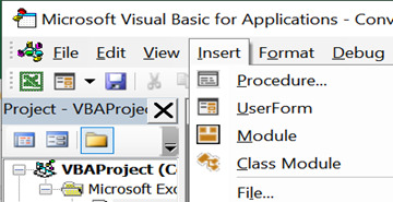
Step 5: Copy the VBA code below and Paste it on Macro Visual Basic Module.

Step 6: Press F5 or the Play button to run the task and generate report as shown in the example above.

Explanation of the VBA Code

The VBA code shown above is further explained below for the users to understand so that they can customize it themselves if they want the result to be different as per their needs.

   ActiveCell.Offset(0, 2).Columns(“A:A”).EntireColumn.Select

The first layer is simply the Offset function which directs excel to move from one cell to the other based on a specific row and column number. In the beginning, the pre-defined excel cell will be the Cell A1. So, from the Syntax, we are telling excel to move zero rows and two columns forward from the cell A1. Once excel moves to cell C1, we are asking it to select the entire column.

   Selection.Copy

The second layer is instructing excel to copy the selected column.

   ActiveCell.Offset(0, 7).Range(“A1”).Select

In the third layer, we are again using the offset function. Please note, that in this case, the Active Cell has now changed to C1 because of previous selection. After moving seven columns forward from the cell, the new active cell will be the cell J1.

   ActiveSheet.Paste

The fourth layer is instructing excel to paste the copied column on the new active cell.

   ActiveSheet.Range(“J:J”).RemoveDuplicates Columns:=1, Header:=xlYes

The fifth layer is the remove duplicates function. We are simply selecting the entire Column J and removing the duplicate values. The Syntax is also defining that the data for remove duplicates is in one column and it contains a header as well.

  ActiveCell.Offset(0, 1).Range(“A1”).Select

The sixth layer is simply the offset function to select cell K1.

   ActiveCell.FormulaR1C1 = “Total Units Sold”

In seventh layer, we type the header.

   ActiveCell.Offset(1, 0).Range(“A1”).Select

In the eight layer, we are instructing excel to move one row downwards.

   ActiveCell.FormulaR1C1 = “=SUMIF(C[-8],RC[-1],C[-6])”

In the ninth layer, we can see that now the active cell is K2. The code simply enters the SUM IF  formulae where it selects the Column C having the representative names and Column E having the total units sold. The negative numbers represent corresponding column distance from selected cell. Leftward or upward cell movements are represented by a negative sign.

   ActiveCell.Select

   Selection.Copy

   ActiveCell.Offset(1, 0).Range(“A1:A10”).Select

   Selection.PasteSpecial Paste:=xlPasteAll, Operation:=xlNone, SkipBlanks:= _

       False, Transpose:=False

The Last part of the code is simply copying the SUM IF formulae to the rest of the representative names to give the result next to each representative name.

Now that you understand how the VBA Code works to automate database reports, you can also customize it as per your needs.

I hope that helps. Please leave a comment below with any questions or suggestions. For more in-depth Excel training, checkout our Ultimate Excel Training Course here. Thank you!