unnatikoppikar

[unnatikoppikar]

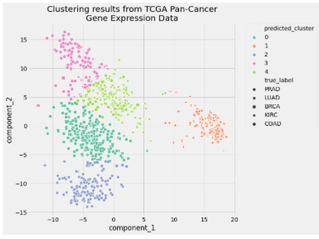
Building a K-Means Clustering Pipeline

What Is Clustering?

Clustering is a set of techniques used to partition data into groups, or clusters. Clusters are loosely defined as groups of data objects that are more similar to other objects in their cluster than they are to data objects in other clusters. In practice, clustering helps identify two qualities of data:

Meaningfulness

Usefulness

There  are three popular categories of clustering algorithms:

Partitional clustering

Hierarchical clustering

Density-based clustering

In [1]: import tarfile

  ...: import urllib   ...:   ...: import numpy as np   ...: import matplotlib.pyplot as plt   ...: import pandas as pd   ...: import seaborn as sns   ...:   ...: from sklearn.cluster import KMeans   ...: from sklearn.decomposition import PCA   ...: from sklearn.metrics import silhouette_score, adjusted_rand_score   ...: from sklearn.pipeline import Pipeline   ...: from sklearn.preprocessing import LabelEncoder, MinMaxScaler In [2]: uci_tcga_url = "https://archive.ics.uci.edu/ml/machine-learning-databases/00401/"   ...: archive_name = "TCGA-PANCAN-HiSeq-801x20531.tar.gz"   ...: # Build the url   ...: full_download_url = urllib.parse.urljoin(uci_tcga_url, archive_name)   ...:   ...: # Download the file   ...: r = urllib.request.urlretrieve (full_download_url, archive_name)   ...: # Extract the data from the archive   ...: tar = tarfile.open(archive_name, "r:gz")   ...: tar.extractall()   ...: tar.close()

In [3]: datafile = "TCGA-PANCAN-HiSeq-801x20531/data.csv"   ...: labels_file = "TCGA-PANCAN-HiSeq-801x20531/labels.csv"   ...:   ...: data = np.genfromtxt(   ...:     datafile,   ...:     delimiter=",",   ...:     usecols=range(1, 20532),   ...:     skip_header=1   ...: )   ...:   ...: true_label_names = np.genfromtxt(   ...:     labels_file,   ...:     delimiter=",",   ...:     usecols=(1,),   ...:     skip_header=1,   ...:     dtype="str"   ...: )

In [4]: data[:5, :3] Out[4]: array([[0.        , 2.01720929, 3.26552691],       [0.        , 0.59273209, 1.58842082],       [0.        , 3.51175898, 4.32719872],       [0.        , 3.66361787, 4.50764878],       [0.        , 2.65574107, 2.82154696]]) In [5]: true_label_names[:5] Out[5]: array(['PRAD', 'LUAD', 'PRAD', 'PRAD', 'BRCA'], dtype='<U4') In [6]: label_encoder = LabelEncoder() In [7]: true_labels = label_encoder.fit_transform(true_label_names) In [8]: true_labels[:5] Out[8]: array([4, 3, 4, 4, 0]) In [9]: label_encoder.classes_ Out[9]: array(['BRCA', 'COAD', 'KIRC', 'LUAD', 'PRAD'], dtype='<U4') In [10]: n_clusters = len(label_encoder.classes_)

In [11]: preprocessor = Pipeline(   ...:     [   ...:         ("scaler", MinMaxScaler()),   ...:         ("pca", PCA(n_components=2, random_state=42)),   ...:     ]   ...: ) In [12]: clusterer = Pipeline(   ...:    [   ...:        (   ...:            "kmeans",   ...:            KMeans(   ...:                n_clusters=n_clusters,   ...:                init="k-means++",   ...:                n_init=50,   ...:                max_iter=500,   ...:                random_state=42,   ...:            ),   ...:        ),   ...:    ]   ...: )

In [13]: pipe = Pipeline(   ...:     [   ...:         ("preprocessor", preprocessor),   ...:         ("clusterer", clusterer)   ...:     ]   ...: ) In [14]: pipe.fit(data) Out[14]: Pipeline(steps=[('preprocessor',                 Pipeline(steps=[('scaler', MinMaxScaler()),                                 ('pca',                                  PCA(n_components=2, random_state=42))])),                ('clusterer',                 Pipeline(steps=[('kmeans',                                  KMeans(max_iter=500, n_clusters=5, n_init=50,                                         random_state=42))]))])

In [15]: preprocessed_data = pipe["preprocessor"].transform(data) In [16]: predicted_labels = pipe["clusterer"]["kmeans"].labels_ In [17]: silhouette_score(preprocessed_data, predicted_labels) Out[17]: 0.5118775528450304 In [18]: adjusted_rand_score(true_labels, predicted_labels) Out[18]: 0.722276752060253 In [19]: pcadf = pd.DataFrame(   ...:     pipe["preprocessor"].transform(data),   ...:     columns=["component_1", "component_2"],   ...: )   ...:   ...: pcadf["predicted_cluster"] = pipe["clusterer"]["kmeans"].labels_   ...: pcadf["true_label"] = label_encoder.inverse_transform(true_labels) In [20]: plt.style.use("fivethirtyeight")   ...: plt.figure(figsize=(8, 8))   ...:   ...: scat = sns.scatterplot(   ...:     "component_1",   ...:     "component_2",   ...:     s=50,   ...:     data=pcadf,   ...:     hue="predicted_cluster",   ...:     style="true_label",   ...:     palette="Set2",   ...: )   ...:   ...: scat.set_title(   ...:     "Clustering results from TCGA Pan-Cancer\nGene Expression Data"   ...: )   ...: plt.legend(bbox_to_anchor=(1.05, 1), loc=2, borderaxespad=0.0)   ...:   ...: plt.show()

[unnatikoppikar]

Lasso Regression

Regression is a modeling task that involves predicting a numeric value given an input.

Lasso Regression

Linear regression refers to a model that assumes a linear relationship between input variables and the target variable.

With a single input variable, this relationship is a line, and with higher dimensions, this relationship can be thought of as a hyperplane that connects the input variables to the target variable. The coefficients of the model are found via an optimization process that seeks to minimize the sum squared error between the predictions (yhat) and the expected target values (y).

loss = sum i=0 to n (y_i – yhat_i)^2

Example of Lasso Regression

In this section, we will demonstrate how to use the Lasso Regression algorithm.

First, let’s introduce a standard regression dataset. We will use the housing dataset.

The housing dataset is a standard machine learning dataset comprising 506 rows of data with 13 numerical input variables and a numerical target variable.

Using a test harness of repeated stratified 10-fold cross-validation with three repeats, a naive model can achieve a mean absolute error (MAE) of about 6.6. A top-performing model can achieve a MAE on this same test harness of about 1.9. This provides the bounds of expected performance on this dataset.

The dataset involves predicting the house price given details of the house suburb in the American city of Boston.

Housing Dataset (housing.csv)

Housing Description (housing.names)

 Sample Code

# load and summarize the housing dataset from pandas import read_csv from matplotlib import pyplot # load dataset url = 'https://raw.githubusercontent.com/jbrownlee/Datasets/master/housing.csv' dataframe = read_csv(url, header=None) # summarize shape print(dataframe.shape) # summarize first few lines print(dataframe.head())

# define modelmodel = Lasso(alpha=1.0)

# evaluate an lasso regression model on the dataset from numpy import mean from numpy import std from numpy import absolute from pandas import read_csv from sklearn.model_selection import cross_val_score from sklearn.model_selection import RepeatedKFold from sklearn.linear_model import Lasso # load the dataset url = 'https://raw.githubusercontent.com/jbrownlee/Datasets/master/housing.csv' dataframe = read_csv(url, header=None) data = dataframe.values X, y = data[:, :-1], data[:, -1] # define model model = Lasso(alpha=1.0) # define model evaluation method cv = RepeatedKFold(n_splits=10, n_repeats=3, random_state=1) # evaluate model scores = cross_val_score(model, X, y, scoring='neg_mean_absolute_error', cv=cv, n_jobs=-1) # force scores to be positive scores = absolute(scores) print('Mean MAE: %.3f (%.3f)' % (mean(scores), std(scores)))

# make a prediction with a lasso regression model on the dataset from pandas import read_csv from sklearn.linear_model import Lasso # load the dataset url = 'https://raw.githubusercontent.com/jbrownlee/Datasets/master/housing.csv' dataframe = read_csv(url, header=None) data = dataframe.values X, y = data[:, :-1], data[:, -1] # define model model = Lasso(alpha=1.0) # fit model model.fit(X, y) # define new data row = [0.00632,18.00,2.310,0,0.5380,6.5750,65.20,4.0900,1,296.0,15.30,396.90,4.98] # make a prediction yhat = model.predict([row]) # summarize prediction print('Predicted: %.3f' % yhat)

[unnatikoppikar]

Random Forest

The random forest is a model made up of many decision trees. Rather than just simply averaging the prediction of trees (which we could call a “forest”), this model uses two key concepts that gives it the name random:

Random sampling of training data points when building trees

Random subsets of features considered when splitting nodes

Dataset

The problem we’ll solve is a binary classification task with the goal of predicting an individual’s health. The features are socioeconomic and lifestyle characteristics of individuals and the label is 0 for poor health and 1 for good health. This dataset was collected by the Centers for Disease Control and Prevention.  Generally, 80% of a data science project is spent cleaning, exploring, and making features out of the data. However, for this article, we’ll stick to the modeling.

Code

from sklearn.ensemble import RandomForestClassifier from sklearn.metrics import roc_auc_score # Create the model with 100 trees model = RandomForestClassifier(n_estimators=100,                               bootstrap = True,                               max_features = 'sqrt') # Fit on training data model.fit(train, train_labels)

# Actual class predictions rf_predictions = model.predict(test) # Probabilities for each class rf_probs = model.predict_proba(test)[:, 1]

# Calculate roc auc roc_value = roc_auc_score(test_labels, rf_probs)

Result