#Method of separation of variables for solving partial differential equations | Explore Tumblr posts and blogs

foxspain82 · 4 years ago

Text

10.4 Usubstitution Trig Functionsap Calculus

10.4 U-substitution Trig Functionsap Calculus Answers

10.4 U-substitution Trig Functionsap Calculus Pdf

10.4 U-substitution Trig Functionsap Calculus Problems

10.4 U-substitution Trig Functionsap Calculus Worksheet

Calculus II, Section 7.4, #67 Integration of Rational Functions by Partial Fractions One method of slowing the growth of an insect population without the use of pesticides is to introduce into the population a number of sterile males that mate with fertile females but produce no o spring. Let P represeent. AP Calculus AB Mu Alpha Theta Welcome to AP Calculus AB! Contact me here. Need more review? Browse the Algebra II and Pre-Calculus Tabs. AP ® Calculus AB and BC. COURSE AND EXAM DESCRIPTION. AP COURSE AND EXAM DESCRIPTIONS ARE UPDATED PERIODICALLY. Please visit AP Central. Mathematics 104—Calculus, Part I (4h, 1 CU) Course Description: Brief review of High School Calculus, methods and applications of integration, infinite series, Taylor's theorem, first order ordinary differential equations. Use of symbolic manipulation and graphics software in Calculus. Note: This course uses Maple®.

Math 104: Calculus I – Notes

Section 004 - Spring 2014

10.4 U-substitution Trig Functionsap Calculus Answers

Syllabus

Concept Videos

Skeleton NotesComplete Notes Title More Remainder 10.6, 10.9 Remainder 10.6/10.9 Series Estimation & Remainder Sections 10.8-10.10 Sections 10.8-10.10 Taylor (and Maclaurin) Series Section 10.7 Section 10.7 Power Series Introduction Section 10.6 Section 10.6 Alt. Series Test and Abs. Conv. Conv. Tests Section 10.5 Section 10.5 The Ratio and Root Tests Section 10.4 Section 10.4 The Comparison Tests Section 10.3 Section 10.3 The Integral Test Section 10.2 Section 10.2 Introduction to Series Section 10.1 Section 10.1 Sequences Section 9.2 Section 9.2 Linear Differential Equations Section 7.2 Pt 1Pt 2 Section 7.2 Separable Differential Equations Section 8.8 Section 8.8 Probability and Calculus Odd Ans. Section 8.7 Pt. 1Pt. 2Section 8.7 Improper Integrals L'Hopital Section 8.4 Pt. 1Pt. 2Section 8.4 Partial Fraction Decomposition Section 8.3 Pt. 1Pt. 2Section 8.3 Trig. Substitution Section 8.2 Pt. 1Pt. 2Section 8.2 Integrating Trig. Powers Section 8.1 Pt. 1Pt. 2 Section 8.1 Integration By Parts Section 6.6 Section 6.6 Center of Mass Section 6.4 Section 6.4 Surface Area of Revolution Section 6.3 Section 6.3 Arc Length Section 6.2Section 6.2 Volumes Using Cylindrical Shells Section 6.1 Section 6.1 Volumes Using Cross-Sections disk/washer Review Calc I Review Calc I ReviewLimit, Derivative, and Integral Area b/w CurvesArea b/w Curves Video Example U-substitution Graphs you should know

Print out the skeleton notes before class and bring them to class so that you don't have to write down https://foxspain82.tumblr.com/post/657282647494672384/achievement-unlocked-2watermelon-gaming. Hide paragraph marks in microsoft word for mac. everything said in class. If you miss anything, the complete notes will be posted after class.

10.4 U-substitution Trig Functionsap Calculus Pdf

10.4 U-substitution Trig Functionsap Calculus Problems

10.4 U-substitution Trig Functionsap Calculus Worksheet

Version #1 The course below follows CollegeBoard's Course and Exam Description. Lessons will begin to appear starting summer 2020. BC Topics are listed, but there will be no lessons available for SY 2020-2021

Unit 0 - Calc Prerequisites (Summer Work) 0.1 Summer Packet

Unit 1 - Limits and Continuity 1.1 Can Change Occur at an Instant? 1.2 Defining Limits and Using Limit Notation 1.3 Estimating Limit Values from Graphs 1.4 Estimating Limit Values from Tables 1.5 Determining Limits Using Algebraic Properties (1.5 includes piecewise functions involving limits) 1.6 Determining Limits Using Algebraic Manipulation 1.7 Selecting Procedures for Determining Limits (1.7 includes rationalization, complex fractions, and absolute value) 1.8 Determining Limits Using the Squeeze Theorem 1.9 Connecting Multiple Representations of Limits Mid-Unit Review - Unit 1 1.10 Exploring Types of Discontinuities 1.11 Defining Continuity at a Point 1.12 Confirming Continuity Over an Interval 1.13 Removing Discontinuities 1.14 Infinite Limits and Vertical Asymptotes 1.15 Limits at Infinity and Horizontal Asymptotes 1.16 Intermediate Value Theorem (IVT) Review - Unit 1

Unit 2 - Differentiation: Definition and Fundamental Properties 2.1 Defining Average and Instantaneous Rate of Change at a Point 2.2 Defining the Derivative of a Function and Using Derivative Notation (2.2 includes equation of the tangent line) 2.3 Estimating Derivatives of a Function at a Point 2.4 Connecting Differentiability and Continuity 2.5 Applying the Power Rule 2.6 Derivative Rules: Constant, Sum, Difference, and Constant Multiple (2.6 includes horizontal tangent lines, equation of the normal line, and differentiability of piecewise) 2.7 Derivatives of cos(x), sin(x), e^x, and ln(x) 2.8 The Product Rule 2.9 The Quotient Rule 2.10 Derivatives of tan(x), cot(x), sec(x), and csc(x) Review - Unit 2

Unit 3 - Differentiation: Composite, Implicit, and Inverse Functions 3.1 The Chain Rule 3.2 Implicit Differentiation 3.3 Differentiating Inverse Functions 3.4 Differentiating Inverse Trigonometric Functions 3.5 Selecting Procedures for Calculating Derivatives 3.6 Calculating Higher-Order Derivatives Review - Unit 3

Unit 4 - Contextual Applications of Differentiation 4.1 Interpreting the Meaning of the Derivative in Context 4.2 Straight-Line Motion: Connecting Position, Velocity, and Acceleration 4.3 Rates of Change in Applied Contexts Other Than Motion 4.4 Introduction to Related Rates 4.5 Solving Related Rates Problems 4.6 Approximating Values of a Function Using Local Linearity and Linearization 4.7 Using L'Hopital's Rule for Determining Limits of Indeterminate Forms Review - Unit 4

Unit 5 - Analytical Applications of Differentiation 5.1 Using the Mean Value Theorem 5.2 Extreme Value Theorem, Global Versus Local Extrema, and Critical Points 5.3 Determining Intervals on Which a Function is Increasing or Decreasing 5.4 Using the First Derivative Test to Determine Relative Local Extrema 5.5 Using the Candidates Test to Determine Absolute (Global) Extrema 5.6 Determining Concavity of Functions over Their Domains 5.7 Using the Second Derivative Test to Determine Extrema Mid-Unit Review - Unit 5 5.8 Sketching Graphs of Functions and Their Derivatives 5.9 Connecting a Function, Its First Derivative, and Its Second Derivative (5.9 includes a revisit of particle motion and determining if a particle is speeding up/down.) 5.10 Introduction to Optimization Problems 5.11 Solving Optimization Problems 5.12 Exploring Behaviors of Implicit Relations Review - Unit 5

Unit 6 - Integration and Accumulation of Change 6.1 Exploring Accumulation of Change 6.2 Approximating Areas with Riemann Sums 6.3 Riemann Sums, Summation Notation, and Definite Integral Notation 6.4 The Fundamental Theorem of Calculus and Accumulation Functions 6.5 Interpreting the Behavior of Accumulation Functions Involving Area Mid-Unit Review - Unit 6 6.6 Applying Properties of Definite Integrals 6.7 The Fundamental Theorem of Calculus and Definite Integrals 6.8 Finding Antiderivatives and Indefinite Integrals: Basic Rules and Notation 6.9 Integrating Using Substitution 6.10 Integrating Functions Using Long Division and Completing the Square 6.11 Integrating Using Integration by Parts (BC topic) 6.12 Integrating Using Linear Partial Fractions (BC topic) 6.13 Evaluating Improper Integrals (BC topic) 6.14 Selecting Techniques for Antidifferentiation Review - Unit 6

Unit 7 - Differential Equations 7.1 Modeling Situations with Differential Equations 7.2 Verifying Solutions for Differential Equations 7.3 Sketching Slope Fields 7.4 Reasoning Using Slope Fields 7.5 Euler's Method (BC topic) 7.6 General Solutions Using Separation of Variables 7.7 Particular Solutions using Initial Conditions and Separation of Variables 7.8 Exponential Models with Differential Equations 7.9 Logistic Models with Differential Equations (BC topic) Review - Unit 7

Unit 8 - Applications of Integration 8.1 Average Value of a Function on an Interval 8.2 Position, Velocity, and Acceleration Using Integrals 8.3 Using Accumulation Functions and Definite Integrals in Applied Contexts 8.4 Area Between Curves (with respect to x) 8.5 Area Between Curves (with respect to y) 8.6 Area Between Curves - More than Two Intersections Mid-Unit Review - Unit 8 8.7 Cross Sections: Squares and Rectangles 8.8 Cross Sections: Triangles and Semicircles 8.9 Disc Method: Revolving Around the x- or y- Axis 8.10 Disc Method: Revolving Around Other Axes 8.11 Washer Method: Revolving Around the x- or y- Axis 8.12 Washer Method: Revolving Around Other Axes 8.13 The Arc Length of a Smooth, Planar Curve and Distance Traveled (BC topic) Review - Unit 8

Unit 9 - Parametric Equations, Polar Coordinates, and Vector-Valued Functions (BC topics) 9.1 Defining and Differentiating Parametric Equations 9.2 Second Derivatives of Parametric Equations 9.3 Arc Lengths of Curves (Parametric Equations) 9.4 Defining and Differentiating Vector-Valued Functions 9.5 Integrating Vector-Valued Functions 9.6 Solving Motion Problems Using Parametric and Vector-Valued Functions 9.7 Defining Polar Coordinates and Differentiating in Polar Form 9.8 Find the Area of a Polar Region or the Area Bounded by a Single Polar Curve 9.9 Finding the Area of the Region Bounded by Two Polar Curves Review - Unit 9

Unit 10 - Infinite Sequences and Series (BC topics) 10.1 Defining Convergent and Divergent Infinite Series 10.2 Working with Geometric Series 10.3 The nth Term Test for Divergence 10.4 Integral Test for Convergence 10.5 Harmonic Series and p-Series 10.6 Comparison Tests for Convergence 10.7 Alternating Series Test for Convergence 10.8 Ratio Test for Convergence 10.9 Determining Absolute or Conditional Convergence 10.10 Alternating Series Error Bound 10.11 Finding Taylor Polynomial Approximations of Functions 10.12 Lagrange Error Bound 10.13 Radius and Interval of Convergence of Power Series 10.14 Finding Taylor Maclaurin Series for a Function 10.15 Representing Functions as a Power Series Review - Unit 8

Version #2 The course below covers all topics for the AP Calculus AB exam, but was built for a 90-minute class that meets every other day. Lessons and packets are longer because they cover more material.

Unit 0 - Calc Prerequisites (Summer Work) 0.1 Things to Know for Calc 0.2 Summer Packet 0.3 Calculator Skillz

Unit 1 - Limits 1.1 Limits Graphically 1.2 Limits Analytically 1.3 Asymptotes 1.4 Continuity Review - Unit 1

Unit 2 - The Derivative 2.1 Average Rate of Change 2.2 Definition of the Derivative 2.3 Differentiability (Calculator Required) Review - Unit 2

Unit 3 - Basic Differentiation 3.1 Power Rule 3.2 Product and Quotient Rules 3.3 Velocity and other Rates of Change 3.4 Chain Rule 3.5 Trig Derivatives Review - Unit 3

Unit 4 - More Deriviatvies 4.1 Derivatives of Exp. and Logs 4.2 Inverse Trig Derivatives 4.3 L'Hopital's Rule Review - Unit 4

Unit 5 - Curve Sketching 5.1 Extrema on an Interval 5.2 First Derivative Test 5.3 Second Derivative Test Review - Unit 5

Unit 6 - Implicit Differentiation 6.1 Implicit Differentiation 6.2 Related Rates 6.3 Optimization Review - Unit 6

Unit 7 - Approximation Methods 7.1 Rectangular Approximation Method 7.2 Trapezoidal Approximation Method Review - Unit 7

Unit 8 - Integration 8.1 Definite Integral 8.2 Fundamental Theorem of Calculus (part 1) 8.3 Antiderivatives (and specific solutions) Review - Unit 8

Unit 9 - The 2nd Fundamental Theorem of Calculus 9.1 The 2nd FTC 9.2 Trig Integrals 9.3 Average Value (of a function) 9.4 Net Change Review - Unit 9

Unit 10 - More Integrals 10.1 Slope Fields 10.2 u-Substitution (indefinite integrals) 10.3 u-Substitution (definite integrals) 10.4 Separation of Variables Review - Unit 10

Unit 11 - Area and Volume 11.1 Area Between Two Curves 11.2 Volume - Disc Method 11.3 Volume - Washer Method 11.4 Perpendicular Cross Sections Review - Unit 11

0 notes

mathematicianadda · 5 years ago

Text

New Wolfram Language Books on Wolfram|Alpha, Calculus, Applied Engineering and System Modeler https://ift.tt/34BjuDD

The pandemic has postponed or canceled a lot of things this year, but luckily learning isn’t one of them. Check out these picks for new Wolfram Language books that will help you explore new software, calculus, engineering and more from the comfort of home.

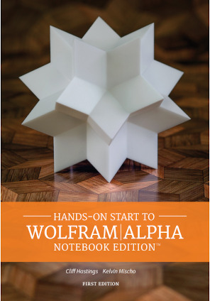
Hands-on Start to Wolfram|Alpha Notebook Edition

New from Wolfram Media and the authors of Hands-on Start to Wolfram Mathematica, Hands-on Start to Wolfram Alpha|Notebook Edition is now available! Wolfram|Alpha Notebook Edition combines the simplicity of Wolfram|Alpha with the computational capabilities of Mathematica for the best of both in a single, unified tool perfect for teaching and learning. Use free-form input to get instant answers to questions, create and customize graphs, and turn static examples into dynamic models. Everything is saved as an interactive Wolfram Notebook, so you can add notes and use notebooks as class or reference materials or present them as dynamic slide shows that engage your audience as you edit examples on the fly.

With this book, you’ll learn how to:

Quickly create notebooks that combine calculations, graphics, interactive examples and notes.

Enter free-form input and get solutions for a variety of calculations (e.g. arithmetic, algebra, calculus, linear algebra).

Access step-by-step solutions, suggestions for next steps and related computations.

Create 2D, 3D and interactive graphics with controls to dynamically change the parameters.

Use previous results in future calculations, assign variables and define functions.

Create dynamic slide show presentations with interactive elements that can be changed on the fly.

Analysis with Mathematica: Volume 1: Single Variable Calculus

In this De Gruyter textbook, Galina Filipuk and Andrzej Kozłowski explore how Mathematica is able to do much more than just numerics. This text shows how to tackle real mathematical problems from basic analysis. Readers will learn how Mathematica represents domains, qualifiers and limits to implement actual proofs—a requirement to unlock the huge potential of Mathematica for a variety of applications. While this volume focuses on single variable calculus, readers should also keep an eye out for Volume 2: Multi-variable Calculus, which is scheduled to be published in 2021.

Symmetry in Optics and Vision Studies: A Data-Analytic Approach

In this book, authors Marlos A. G. Viana and Vasudevan Lakshminarayanan present an introduction to the foundations, interpretations and data-analytic applications of symmetry studies with an emphasis on applications in optical sciences. Symmetry studies connect group theoretic and statistical methods for data summary and inference. This book is written for an audience familiar with calculus and linear algebra as well as introductory statistics. The book reviews finite group theory in the introductory chapters. Computational tools used in the text are also available for download as Mathematica notebooks, offering readers an interactive experience.

Advanced Engineering Mathematics with Mathematica

Advanced Engineering Mathematics with Mathematica presents advanced analytical solution methods that are used to solve boundary value problems in engineering and integrates these methods with Mathematica procedures. In this book, author Edward B. Magrab emphasizes the Sturm–Liouville system and the generation and application of orthogonal functions, which are used by the separation of variables method to solve partial differential equations. It introduces the relevant aspects of complex variables, matrices and determinants, Fourier series and transforms, solution techniques for ordinary differential equations, the Laplace transform and procedures to make ordinary and partial differential equations used in engineering non-dimensional. Magrab presents numerous and widely varied solved boundary value problems to show the diverse applications of the material.

Computer Modeling and Simulation of Dynamic Systems Using Wolfram SystemModeler

Geared toward students and professionals in the field of dynamic system modeling, this book briefly discusses the main provisions of the theory of modeling. It also describes in detail the methodology for constructing computer models of dynamic systems using the Wolfram visual modeling environment, System Modeler, and provides illustrative examples of solving problems of mechanics and hydraulics. This book serves as a supplement to university courses in modeling and simulation of dynamic systems, but it’s also a great resource for anyone looking for examples and explanations of System Modeler.

Applied Engineering Mathematics

This textbook is written for undergraduate engineering students (specifically those in years 2–4 of an engineering degree course) and it places a strong emphasis on visualization and the methods and tools needed across the whole of engineering. Author Brian Vick emphasizes the visual approach while avoiding excessive proofs and derivations. The visual images explain and teach the mathematical methods. The book’s website provides Mathematica notebooks with dynamic and interactive code to accompany the examples for the reader to explore with Mathematica or the free Wolfram Player, and it provides access for instructors to a solutions manual.

If you’re interested in finding more books that use the Wolfram Language, check out the full collection on the Wolfram Books site. If you’re working on a Mathematica or Wolfram Language book, contact us to find out more about our options for author support and to have your book featured in an upcoming blog post!

Get full access to the latest Wolfram Language functionality with a Mathematica 12.1 or Wolfram|One trial.

from Wolfram Blog » Mathematics https://ift.tt/3kGcJGb from Blogger https://ift.tt/2TxwEeG

#Blogger

0 notes

edukiteuk-blog · 6 years ago

Link

This course covers the classical partial differential equations of applied mathematics: diffusion, Laplace/Poisson, and wave equations. It also includes methods and tools for solving these PDEs, such as separation of variables, Fourier series and transforms, eigenvalue problems, and the Wave Equation in One Space Variable.See More: https://bit.ly/2WnH4QZ

0 notes

coursesforallacademynoida · 6 years ago

Text

B.Sc Tuition In Noida For Partial Differential Equations

CFA Academy For B.Sc Maths Tuition Classes In Noida. Linear Algebra Tuition In Noida, Calculus Tuition In Noida, Real Analysis Tuition In Noida, Complex Analysis Tuition In Noida, Ordinary Differential Equations Tuition In Noida, Algebra Tuition In Noida, Functional Analysis Tuition In Noida, Numerical Analysis Tuition In Noida, Partial…

View On WordPress

#Algebra Tuition In Noida #B.Sc Tuition In Noida For Partial Differential Equations #B.Sc Tuition In Noida For Partial Differential Equations CFA Academy For B.Sc Maths Tuition Classes In Noida. Linear Algebra Tuition In Noid #Calculus Tuition In Noida #Complex Analysis Tuition In Noida #Dirichlet and Neumann problems; Solutions of Laplace and wave equations in two dimensional Cartesian coordinates #Functional Analysis Tuition In Noida #interior and exterior Dirichlet problems in polar coordinates; Separation of variables method for solving wave and diffusion equations in on #Linear Programming Tuition In Noida Linear and quasi-linear first order partial differential equations #method of characteristics; Second order linear equations in two variables and their classification; Cauchy #Numerical Analysis Tuition In Noida #Ordinary Differential Equations Tuition In Noida #Partial Differential Equation Tuition In Noida #Real Analysis Tuition In Noida #Topology Tuition In Noida

0 notes

civilengineering-crimson · 5 years ago

Text

Open Journal of Civil Engineering_Crimson Publishers

Analytical Solutions of a Conduction Problem with Two Different Kinds of Boundary Conditions by Zhongzhi Fu in Advancements in Open Journal of Civil Engineering

A heat transfer problem was taken as an example to provide the analytical solutions of a one-dimensional conduction problem with two different kinds of boundary conditions. The theoretical solutions were obtained by using the method of separation of variables for solving partial differential equations. Temperature distribution in two simple cases were studied using the analytical solutions and were compared with corresponding numerical results. Reliability of the analytical results were shown by their excellent agreement with those numerical ones. The solutions presented in this note can be used for the verification of new numerical algorithms.

For more open access journals in Crimson Publishers

please click on the link https://crimsonpublishersresearch.com/

For more articles in Open Journal of Civil Engineering

Please click on the link https://crimsonpublishers.com/acet/

Follow On Linkedin : https://linkedin.com/in/chyler-henley-ba9623175 Follow On Medium : https://medium.com/crimson-publishers/crimson-publishers-journals-f29e22da8f5c

#Open access journal #Peer Review journal of ACET #crimsonpublishers

0 notes

cynthiabryanuk · 7 years ago

Text

Computational Efficiency of Decoupling Approach in Solving Reactive Transport Model: A Case Study of Pyrite Oxidative Dissolution

Geofluids Volume 2017 (2017), Article ID 4670103, 7 pages https://doi.org/10.1155/2017/4670103

Computational Efficiency of Decoupling Approach in Solving Reactive Transport Model: A Case Study of Pyrite Oxidative Dissolution

1State Key Laboratory of Hydrology-Water Resources and Hydraulic Engineering, Nanjing Hydraulic Research Institute, Nanjing 210029, China 2College of Earth Science and Engineering, Hohai University, Nanjing 210098, China

Academic Editor: Keni Zhang

Copyright © 2017 Jixiang Huo et al. This is an open access article distributed under the Creative Commons Attribution License, which permits unrestricted use, distribution, and reproduction in any medium, provided the original work is properly cited.

Abstract

Pyrite existed widely in nature and its oxidative dissolution might lead groundwater to become acidic, which was harmful to the environment and indeed to artificial building materials. The reactive transport model was a useful tool to predict the extent of such pollution. However, the chemical species were coupled together in the form of a reaction term, which might lead the equations to be nonlinear and thus difficult to solve. A decoupling approach was presented: linear algebraic manipulations of the stoichiometric coefficients of the chemical reactions for the purpose of reducing the number of equation variables and simplifying the reactive source were used. Then the original and decoupled models were solved separately, by both a direct solver and an iterative solver. By comparing the solution times of two models, it was shown that the decoupling approach could enhance the computational efficiency, especially in situations using denser meshes. Using a direct solver, more solution time was saved than when using an iterative version.

1. Introduction

Pyrite is a common, naturally occurring mineral. In the open atmosphere pyrite oxidative dissolution occurs under the action of groundwater. On one hand the resulting acid water may cause environmental problems, such as contamination of surface and ground waters directed to urban and agricultural supply [1–3]. Some toxic elements especially, such as arsenic, are closely associated with pyrite. The kinetic oxidative dissolution of As-bearing pyrite due to dissolved oxygen in the ambient groundwater is an important mechanism for arsenic release in groundwater under both natural conditions and engineering applications [4, 5]. On the other hand the formation of acid water also has some impacts on artificial building materials because of sulfate attack and acid attack [6, 7]. All the above lead the management of potentially acid generating waste rock to be very important [8]. To study the extent and scope of acidic water pollution, some hydrogeochemical models and transport ones are developed to simulate such a system [9–11].

In recent years reactive transport model is widely used to simulate the contaminant transport, water-rock interaction, and other processes in earth science fields [12, 13]. To improve computational efficiency of the model, Friedly and Rubin [14] present a general, concise formulation (decoupling approach) by means of linear algebraic manipulations of the stoichiometric coefficients of the chemical reactions, which can reduce the number of unknown variables and simplify the reaction source/sink terms. Based on this, De Simoni et al. [15] and Molins and Mayer [16] build up the decoupling matrix according to the equilibrium and kinetic reactions. And Huo et al. [17] extend its applications to heterogeneous media. Some efficiency tests are done by Kräutle and Knabner [18] and Hoffmann et al. [19] to study the resulting improvement. In recent years, the decoupling approach is widely used in both engineering applications and laboratory experiments. Saaltink et al. [20] apply the approach into the modelling of multiphase flow for CO2 injection and storage in deep saline aquifers. And the approach is also used in the simulation of two-phase multicomponent flow with reactive transport in porous media [21, 22]. And in identifying geochemical processes using end member mixing analysis, Pelizardi et al. [23] uses the decoupling approach to help in the identification of both end members and such reactions, so as to improve mixing ratio calculations. In laboratory experiments and its simulation, the approach is applied in a laboratory experiment where a sand column saturated with a MgSO4 solution is subject to evaporation [24]. And some programs and models are built up based on the decoupling approach for hydrogeochemical calculations, such as CHEPROO++ [25] and MRWM [26].

In this paper, a reactive transport model of pyrite oxidative dissolution is built up in COMSOL Multiphysics, a finite element software platform for the simulation of physics-based problems. COMSOL is a multiphysics modelling tool that solves various coupled physical problems based on Finite Element Analysis and Partial Differential Equations. It provides a user-friendly interface for mesh generation, equations configuration, and results visualization. And it is widely applied in earth science field. For example, Shao et al. [27] uses it to couple a dual-permeability model with a soil mechanics model for landslide stability evaluation on a hillslope scale. Azad et al. [28] build up an interface between COMSOL and GEMS, a chemical modelling platform, for the reactive transport modelling in variably saturated porous media, while Nardi et al. [29] and Jara et al. [30] couple two standalone simulation programs, COMSOL and PHREEQC, for the reactive transport modelling.

Although some studies have been done on computational efficiency, they are carried out from different research directions. Hoffmann et al. [19] mainly study the impact from theory view, while Kräutle and Knabner’ work [18] is based on a transient model to study computational efficiency in different time steps of two approaches. In this paper, we focused on the number of meshes and different solvers. Based on a brief introduction to the theories and mathematical methods behind the decoupling approach, a reactive transport model of pyrite oxidative dissolution is solved by a traditional method and a decoupling approach separately to compare their computational efficiencies. In both 1D and 2D models, the study area is meshed to different grid refinements in each situation. The original and decoupled models are solved and their solution times are compared. Meanwhile, the 2D models are solved by both a direct and an iterative solver to study the effect on the computational efficiency of the decoupling approach compared to different solvers. It is aimed at providing a more convenient and efficient method of calculation to solve the reactive transport model of pyrite oxidative dissolution.

2. Mathematical Description

The chemical reactions involved in aqueous species are divided into two kinds, equilibrium reaction and kinetic one. Reaction rates of the former are fast in comparison to transport, so that local chemical equilibrium can be assumed at every point within the system. Kinetic laws are applied to represent the processes of latter one, which is not sufficiently fast enough. So without considering the influence of activity, the mass balance of each species can be written in concise vector notation as follows:where vector contains the mass of species per unit volume of porous medium, and it can be split into two parts, and , respectively, related to the constant activity species (such as minerals in solid phase and gases) and to the remaining species. Matrix is diagonal and its diagonal terms are unity when a given species is mobile and zero otherwise. contains species concentrations in mol/mass of liquid ( for mobile species, is porosity) and , while , are primary and secondary species: the number of secondary species is equal to the number of reaction equilibrium, and the linear operator in (1) is defined as , where is the water flux and D is dispersion coefficient; is a matrix containing the stoichiometric coefficients of reactions involving reactants and product(s) and , where and represent the matrices of equilibrium and kinetic reactions such that due to the primary and secondary species. is stoichiometric coefficients matrix of primary species and is stoichiometric coefficients matrix of secondary species. Vector contains the reaction rate and is also divided into two parts: and .

A full rank matrix, , can be established, orthogonal to , which satisfies . The component matrix can be calculated by means of Gauss-Jordan elimination which leads to the following expression [31]:where is a diagonal matrix of dimension , with all diagonal elements equal to one; and are the number of reactions and species. Now a component vector of is defined as and its number, , can be calculated by . Writing the transport equations in terms of is helpful because the source/sink term becomes simple. Species concentration can also be solved with the equilibrium reaction constants.

According to Molins et al. [32], four types of reactive transport systems are classified by the types of reactions, as shown in Table 1.

Table 1: Types of reactive transport system.

It can be seen that four types of reactive transport systems are classified. The characteristics and calculation of component matrix U of each system are shown as follows.

(1) The first is tank system, in which all reactions take place in equilibrium in the aqueous phase, which means a large aqueous reservoir with residence times long enough for aqueous species to reach equilibrium, and no interaction with other solid or gas phases assumed. The component matrix of this system, , can be calculated by the following equation.where is stoichiometric coefficients matrix of equilibrium reactions corresponding to primary species.

(2) The second is canal system, in which all reactions are homogeneous, but some may be slow (kinetic). The component matrix of this system, , can be calculated by the following equation.where and is stoichiometric coefficients matrix of kinetic reactions corresponding to primary species.

(3) The third is river system, in which heterogeneous reactions also take place, but they are slow relative to flow. The component matrix of this system, , can be calculated by the following equation.where F is a factor matrix which is multiplied by to eliminate the immobile kinetic species. More detailed solution steps of F can be seen in Molins et al. [32].

(4) The fourth is aquifer system, where some heterogeneous reactions are fast enough to be considered in equilibrium. Some fixed activity species (e.g., minerals and H2O) can be found among the equilibrium reactions. These species can be eliminated from the equations by reducing the components to be solved. The component matrix of this system, , can be calculated by the following equation.where E is a factor matrix which is multiplied by to eliminate constant activity species and reduce the number of components. More detailed solution steps of can be seen in Molins et al. [32].

3. Decoupling Approach in Pyrite Oxidative Dissolution

3.1. The Chemical System and Its Decoupling Matrix

It is important to build up a chemical reaction system for pyrite oxidative dissolution reactive transport. When the initial solution is assumed to be formed in deionized water, the main reactions occurring in the open system are as follows.where there are equilibrium reactions in both (7) and (8), with reaction rates of and and (9) reflects the process of pyrite oxidative dissolution, which depends on the concentration of H+ and O2(aq) in solution. According to these, the stoichiometric coefficient matrix of the system S could be written asSince the reactions involved both aqueous and solid phases, it satisfied the aquifer system in Section 2. So the component matrix, , could be calculated asAnd a new vector of components, , was defined aswhere the vector in this system comprised eight species: O2(aq), H+, OH-, , Fe3+, FeS2, O2(g), and H2O in order. The calculated aqueous components were u1, u2, u3. As (12) shows the component vector is a linear combination of species, which is readily calculated; the number of unknowns to be solved in the equations is reduced, from eight species to three components. In this system, the number of all species is defined as , with and the number of equilibrium reactions is 2, while the number of secondary species with fixed activity is defined as , which includes pyrite, H2O, and O2(g). In this system , so the number of components, , could be calculated as

Meanwhile, the reaction terms of species in the transport equations were as follows:Multiplying by the decoupling matrix, U, this term could be expressed asIt could be seen that the reaction term of the original model was more complicated and contained the expressions of the equilibrium reaction rates R1 and R2, both of which were difficult to obtain explicitly which introduced some difficulties when solving the model. However, it was expressed in the form of extremely simple items by means of the decoupling approach. As shown in (15), the reaction terms of components, u1 and u2, were 0, and the one of component u3 involved only R3. Then the transport equations of component could be solved. Once system components had been evaluated, the original species, c, was obtained from the nonlinear algebraic system of (12) and corresponding equilibrium constants of (7) and (8).

3.2. Verification

In order to verify the influence of the decoupling approach on the calculation accuracy, firstly a batch reactor system of pyrite oxidation dissolution was taken as an example. In this system the pyrite was completely immersed in deionized water in a stirred vessel, which meant there was no need to consider the transport problem. The simulation results by both original approach and decoupling one were compared. The chemical parameters are shown in Table 2.

Table 2: Chemical parameters of pyrite oxidation dissolution.

and are the equilibrium constant of (7) and (8), while ,, and are reaction parameters of pyrite oxidative dissolution. Its reaction rate could be calculated by the following equation.where is solid phase surface area and is water volume; and are concentration of O2(aq) and H+.

The ratio of solid phase surface area to water volume was set as 3 dm−1 and simulated time was 10 days. The variation and error of pH value and Fe3+ concentration in two models are shown in Figure 1.

Figure 1: Variation and error of pH value and Fe3+ concentration.

It can be seen from Figure 1 that the results of two models are basically the same. Maximum relative error of pH value is −0.04725%, while the one of Fe3+ is 0.59542%, which means that decoupling approach has little effect on the accuracy of the calculation.

3.3. Comparison of Computational Efficiency

The decoupling approach not only simplified the reaction term but also reduced the number of unknown variables in the transport equations. As a result, the new transport model of each component should now be solvable with improved computational efficiency. Deionized water flows through a single smooth fracture of pyrite can be simplified to either a 1D or 2D parallel plate model with model parameters as shown in Table 3.

Table 3: Parameters for the 1D and 2D models.

Initially the fracture was deemed to have been full of deionized water, with a constant flow velocity through the fracture. Without considering the change in the aperture size caused by dissolution, the distribution of aqueous species reached dynamic equilibrium, which can be regarded as a steady state. The two models were thus simulated. One of the two models involved transport of species and the original model was designated: the other involved transport of decoupled component and the decoupled model was designated.

Then the two models were separately established in COMSOL 3.5a, a software platform for the simulation of physics-based problems. The central processing unit (CPU) of the computer was an Intel Core Duo P8400 with a clock speed of 2.26 GHz and the motherboard had 3 GB of random access memory. There were two main categories of solver in the software: direct and iterative. The former included UMFPACK, SPOOLES, PARDISO, and TAUCS Cholesky, which solved a linear system by Gaussian elimination. The iterative solvers, GMRES, FGMRES, conjugate gradients, BiCGStab, and geometric multigrid, were more memory-efficient to deal with models with many degrees of freedom.

When the model was solved in COMSOL, the mesh generator partitioned the study domains into mesh elements: the number of elements depended on the maximum element size when they were uniformly subdivided. Then the 1D and 2D models (original and decoupled types) were solved separately. First the direct solver, UMFPACK, was chosen and the model was solved three times in each case. To solve the nonlinear equations in both original model and decoupled one, Damped Newton Method (DNM) was adopted. Relative tolerance was set as 1.0 × 10−6 and maximum number of iterations was set as 25. The average solution times are shown in Tables 4 and 5.

Table 4: Comparison of solution time in 1D model using direct solver, UMFPACK.

Table 5: Comparison of solution time in 2D model using direct solver, UMFPACK.

It can be seen from Tables 4 and 5 that:

(1) Solution by direct solver, UMFPACK, costs much more time in the original model than when adopting a decoupling approach in both 1D and 2D models.

(2) The solution time in both 1D models increases with the number of elements, but it saves more time by using a decoupling approach when the number of elements becomes large. When there are only 25 elements in the model, it costs 0.234 s and 0.094 s to solve each model. With the increase in the number of elements, the solution times reach 1.079 s and 0.297 s for 500 elements (some 4.61 and 3.16 times the requirements at 25 elements).

(3) As in 1D, the computing time in 2D also increases with the number of elements in both of the two models and it saves more time when using a decoupling approach for large numbers of elements. At 7,800 elements, the original model cannot be solved due to an out of memory error during LU factorisation. However, by using a decoupling approach it only costs 21.033 s. Compared to the 1D model, it has a better computational efficiency costing only 4.78% to 27.71% of the original.

Then the iterative solver GMRES was chosen to solve the 2D model. The solution set of nonlinear equations was the same as the direct solver, UMFPACK. Three replicates were run and the average solution times are shown in Table 6.

Table 6: Comparison of solution time in 2D model using iterative solver, GMRES.

The following can be seen from Table 6.

(1) Like the results in Table 3, the decoupling approach also enhances the computational efficiency when solving the two models by use of the iterative solver. The decoupled solution time is only 17.92% to 52.34% of that needed for the original model and the solution time increases with the number of elements no matter whether in the original or decoupled model.

(2) Unlike the situation in Table 3, does not reduce with increased numbers of elements: at 5,036 and 7,800 elements, is only 51.54% and 52.34% of that required originally. It shows that the decoupling approach does not have as significant an effect as expected when used iteratively on a large model.

(3) Solving the original model with a direct solver costs much more time than when using an iterative version. However, when dealing with a decoupled model, the direct solver is faster and (Table 3) ranges from 4.78% to 27.71%, while it is 17.92% to 52.34% in Table 4. This means that solving the decoupled model by using an iterative solver does not save as much time as the direct solver does.

According to Tables 5 and 6, solution times for original and decoupled models with direct and iterative solvers are shown in Figure 2.

Figure 2: Comparison of solution times.

Figure 2 shows that solving an original model takes more time than a decoupled one, no matter whether by direct solver or iterative solver. In general sorted by time taken: the decoupled model by direct solver < decoupled model by iterative solver < original model by iterative solver < original model by direct solver.

4. Conclusions

The present work described the basic theory and mathematical methods of the decoupling approach and then took pyrite oxidative dissolution as an example. Based on the analysis of its chemical reaction system, the decoupling matrix U was calculated. When multiplied by U, the concentration vector was converted to the component vector , which had fewer variables and simpler reaction terms. Then the original and decoupled models were established in COMSOL Multiphysics 3.5a. Then the study domain was meshed at different degrees of refinement. In each case it was solved by direct and iterative solvers. The results show the following.

(1) Decoupling enhances the computational efficiency in both 1D and 2D models while saving more time for 2D models than 1D models.

(2) The more mesh grids the domain generates, the more efficiently the decoupled model finds a solution by direct solver, whether in 1D or 2D.

(3) Although the iterative solver takes less time than the direct solver for the original 2D model, it is more efficient to use a direct solver in solving a decoupled problem.

(4) The solution times in ascending order are the decoupled model solved by direct solver, a decoupled model solved by an iterative solver, the original model solved by an iterative solver, and the original model solved by a direct solver.

As a conclusion, the decoupling approach is of assistance when solving reactive transport of pyrite oxidative dissolution problems, especially over a large domain with more mesh elements. Its applicability is thus demonstrated.

Conflicts of Interest

The authors declare that there are no conflicts of interest regarding the publication of this article.

Acknowledgments

This work was supported by Young Scientists Fund of the National Natural Science Foundation of China (Grant no. 51609150), the China Postdoctoral Science Foundation (Grant no. 2016M590477), the National Natural Science Foundation of China (Grant no. 41272265), and the Special Scientific Research Fund of Public Welfare Profession of Ministry of Water Resources of China (Grants nos. 201501033 and 201501036).

References

J. A. Grande, R. Beltrán, A. Sáinz, J. C. Santos, M. L. De La Torre, and J. Borrego, “Acid mine drainage and acid rock drainage processes in the environment of Herrerías Mine (Iberian Pyrite Belt, Huelva-Spain) and impact on the Andevalo Dam,”Environmental Geology, vol. 47, no. 2, pp. 185–196, 2005.View at Publisher·View at Google Scholar·View at Scopus

J. A. Grande, M. Santisteban, M. L. de la Torre, T. Valente, and E. Pérez-Ostalé, “Characterisation of AMD Pollution in the Reservoirs of the Iberian Pyrite Belt,”Mine Water and the Environment, vol. 32, no. 4, pp. 321–330, 2013.View at Publisher·View at Google Scholar·View at Scopus

P. M. Heikkinen, M. L. Räisänen, and R. H. Johnson, “Geochemical characterisation of seepage and drainage water quality from two sulphide mine tailings impoundments: Acid mine drainage versus neutral mine drainage,”Mine Water and the Environment, vol. 28, no. 1, pp. 30–49, 2009.View at Publisher·View at Google Scholar·View at Scopus

M. M. Rahman, M. Bakker, C. H. L. Patty et al., “Reactive transport modeling of subsurface arsenic removal systems in rural Bangladesh,”Science of the Total Environment, vol. 537, pp. 277–293, 2015.View at Publisher·View at Google Scholar·View at Scopus

S. Fakhreddine, J. Lee, P. K. Kitanidis, S. Fendorf, and M. Rolle, “Imaging geochemical heterogeneities using inverse reactive transport modeling: An example relevant for characterizing arsenic mobilization and distribution,”Advances in Water Resources, vol. 88, pp. 186–197, 2016.View at Publisher·View at Google Scholar·View at Scopus

A. Rodrigues, J. Duchesne, B. Fournier, B. Durand, P. Rivard, and M. Shehata, “Mineralogical and chemical assessment of concrete damaged by the oxidation of sulfide-bearing aggregates: Importance of thaumasite formation on reaction mechanisms,”Cement and Concrete Research, vol. 42, no. 10, pp. 1336–1347, 2012.View at Publisher·View at Google Scholar·View at Scopus

T. Schmidt, A. Leemann, E. Gallucci, and K. Scrivener, “Physical and microstructural aspects of iron sulfide degradation in concrete,”Cement and Concrete Research, vol. 41, no. 3, pp. 263–269, 2011.View at Publisher·View at Google Scholar·View at Scopus

M. F. Lengke, A. Davis, and C. Bucknam, “Improving management of potentially acid generating waste rock,”Mine Water and the Environment, vol. 29, no. 1, pp. 29–44, 2010.View at Publisher·View at Google Scholar·View at Scopus

C. Kohfahl and A. Pekdeger, “Rising groundwater tables in partly oxidized pyrite bearing dump-sediments: Column study and modelling approach,”Journal of Hydrology, vol. 331, no. 3-4, pp. 703–718, 2006.View at Publisher·View at Google Scholar·View at Scopus

B. Blunden and B. Indraratna, “Pyrite oxidation model for assessing ground-water management strategies in acid sulfate soils,”Journal of Geotechnical and Geoenvironmental Engineering, vol. 127, no. 2, pp. 146–157, 2001.View at Publisher·View at Google Scholar·View at Scopus

R. Abbassi, F. Khan, and K. Hawboldt, “Prediction of minerals producing acid mine drainage using a computer-assisted thermodynamic chemical equilibrium model,”Mine Water and the Environment, vol. 28, no. 1, pp. 74–78, 2009.View at Publisher·View at Google Scholar·View at Scopus

C. I. Steefel, D. J. DePaolo, and P. C. Lichtner, “Reactive transport modeling: An essential tool and a new research approach for the Earth sciences,”Earth and Planetary Science Letters, vol. 240, no. 3-4, pp. 539–558, 2005.View at Publisher·View at Google Scholar·View at Scopus

C. I. Steefel, C. A. Appelo, and B. Arora, “Reactive transport codes for subsurface environmental simulation,”Computational Geosciences, vol. 19, no. 3, pp. 445–478, 2015.View at Publisher·View at Google Scholar·View at MathSciNet

J. C. Friedly and J. Rubin, “Solute transport with multiple equilibrium‐controlled or kinetically controlled chemical reactions,”Water Resources Research, vol. 28, no. 7, pp. 1935–1953, 1992.View at Publisher·View at Google Scholar·View at Scopus

M. De Simoni, J. Carrera, X. Sánchez-Vila, and A. Guadagnini, “A procedure for the solution of multicomponent reactive transport problems,”Water Resources Research, vol. 41, no. 11, Article ID W11410, pp. 1–16, 2005.View at Publisher·View at Google Scholar·View at Scopus

S. Molins and K. U. Mayer, “Coupling between geochemical reactions and multicomponent gas and solute transport in unsaturated media: A reactive transport modeling study,”Water Resources Research, vol. 43, no. 5, Article ID W05435, 2007.View at Publisher·View at Google Scholar·View at Scopus

J.-X. Huo, H.-Z. Song, and Z.-W. Wu, “Multi-component reactive transport in heterogeneous media and its decoupling solution,”Journal of Contaminant Hydrology, vol. 166, pp. 11–22, 2014.View at Publisher·View at Google Scholar·View at Scopus

S. Kräutle and P. Knabner, “A new numerical reduction scheme for fully coupled multicomponent transport-reaction problems in porous media,”Water Resources Research, vol. 41, no. 9, Article ID W09414, pp. 1–17, 2005.View at Publisher·View at Google Scholar·View at Scopus

J. Hoffmann, S. Kräutle, and P. Knabner, “A general reduction scheme for reactive transport in porous media,”Computational Geosciences, vol. 16, no. 4, pp. 1081–1099, 2012.View at Publisher·View at Google Scholar·View at MathSciNet

M. W. Saaltink, V. Vilarrasa, F. De Gaspari, O. Silva, J. Carrera, and T. S. Rötting, “A method for incorporating equilibrium chemical reactions into multiphase flow models for CO2 storage,”Advances in Water Resources, vol. 62, pp. 431–441, 2013.View at Publisher·View at Google Scholar·View at Scopus

E. Ahusborde, M. Kern, and V. Vostrikov, “Numerical simulation of two-phase multicomponent flow with reactive transport in porous media: application to geological sequestration of CO2,” in Proceedings of the ESAIM: Proceedings and Surveys, vol. 50, pp. 21–39.

E. Ahusborde and M. El Ossmani, “A sequential approach for numerical simulation of two-phase multicomponent flow with reactive transport in porous media,”Mathematics and Computers in Simulation, vol. 137, pp. 71–89, 2017.View at Publisher·View at Google Scholar·View at MathSciNet·View at Scopus

F. Pelizardi, S. A. Bea, J. Carrera, and L. Vives, “Identifying geochemical processes using End Member Mixing Analysis to decouple chemical components for mixing ratio calculations,”Journal of Hydrology, vol. 550, pp. 144–156, 2017.View at Publisher·View at Google Scholar

P. Gamazo, M. W. Saaltink, J. Carrera, L. Slooten, S. A. Bea, and M. Gran, “Modeling the influence of MgSO4 invariant points on multiphase reactive transport process during saline soil evaporation,”Physics and Chemistry of the Earth, vol. 64, pp. 57–64, 2013.View at Publisher·View at Google Scholar·View at Scopus

F. d. Gaspari, “Mixing and speciation algorithms for geochemical and reactive transport problems,” 2015.

J. Soler-Sagarra, L. Luquot, L. Martínez-Pérez, M. W. Saaltink, F. De Gaspari, and J. Carrera, “Simulation of chemical reaction localization using a multi-porosity reactive transport approach,”International Journal of Greenhouse Gas Control, vol. 48, pp. 59–68, 2016.View at Publisher·View at Google Scholar·View at Scopus

W. Shao, T. Bogaard, and M. Bakker, “How to Use COMSOL Multiphysics for Coupled Dual-permeability Hydrological and Slope Stability Modeling,”Procedia Earth and Planetary Science, vol. 9, pp. 83–90, 2014.View at Publisher·View at Google Scholar

V. J. Azad, C. Li, C. Verba, J. H. Ideker, and O. B. Isgor, “A COMSOL-GEMS interface for modeling coupled reactive-transport geochemical processes,”Computers & Geosciences, vol. 92, pp. 79–89, 2016.View at Publisher·View at Google Scholar·View at Scopus

A. Nardi, A. Idiart, P. Trinchero, L. M. De Vries, and J. Molinero, “Interface COMSOL-PHREEQC (iCP), an efficient numerical framework for the solution of coupled multiphysics and geochemistry,”Computers & Geosciences, vol. 69, pp. 10–21, 2014.View at Publisher·View at Google Scholar·View at Scopus

D. Jara, J.-R. d. Dreuzy, and B. Cochepin, “TReacLab, An object-oriented implementation of non-intrusive splitting methods to couple independent transport and geochemical software,”Computers & Geosciences.

M. W. Saaltink, C. Ayora, and J. Carrera, “A mathematical formulation for reactive transport that eliminates mineral concentrations,”Water Resources Research, vol. 34, no. 7, pp. 1649–1656, 1998.View at Publisher·View at Google Scholar·View at Scopus

S. Molins, J. Carrera, C. Ayora, and M. W. Saaltink, “A formulation for decoupling components in reactive transport problems,”Water Resources Research, vol. 40, no. 10, pp. W103011–W1030113, 2004.View at Publisher·View at Google Scholar·View at Scopus

Source

http://www.hindawi.com/journals/geofluids/2017/4670103/

from http://taxi.nearme.host/computational-efficiency-of-decoupling-approach-in-solving-reactive-transport-model-a-case-study-of-pyrite-oxidative-dissolution/

from NOVACAB - Blog http://novacabtaxi.weebly.com/blog/computational-efficiency-of-decoupling-approach-in-solving-reactive-transport-model-a-case-study-of-pyrite-oxidative-dissolution

0 notes

novacabtaxi · 7 years ago

Text

Computational Efficiency of Decoupling Approach in Solving Reactive Transport Model: A Case Study of Pyrite Oxidative Dissolution

Geofluids Volume 2017 (2017), Article ID 4670103, 7 pages https://doi.org/10.1155/2017/4670103

Computational Efficiency of Decoupling Approach in Solving Reactive Transport Model: A Case Study of Pyrite Oxidative Dissolution

Academic Editor: Keni Zhang

Abstract

1. Introduction

2. Mathematical Description

According to Molins et al. [32], four types of reactive transport systems are classified by the types of reactions, as shown in Table 1.

Table 1: Types of reactive transport system.

It can be seen that four types of reactive transport systems are classified. The characteristics and calculation of component matrix U of each system are shown as follows.

3. Decoupling Approach in Pyrite Oxidative Dissolution

3.1. The Chemical System and Its Decoupling Matrix

3.2. Verification

Table 2: Chemical parameters of pyrite oxidation dissolution.

Figure 1: Variation and error of pH value and Fe3+ concentration.

3.3. Comparison of Computational Efficiency

Table 3: Parameters for the 1D and 2D models.

Table 4: Comparison of solution time in 1D model using direct solver, UMFPACK.

Table 5: Comparison of solution time in 2D model using direct solver, UMFPACK.

It can be seen from Tables 4 and 5 that:

(1) Solution by direct solver, UMFPACK, costs much more time in the original model than when adopting a decoupling approach in both 1D and 2D models.

Table 6: Comparison of solution time in 2D model using iterative solver, GMRES.

The following can be seen from Table 6.

According to Tables 5 and 6, solution times for original and decoupled models with direct and iterative solvers are shown in Figure 2.

Figure 2: Comparison of solution times.

4. Conclusions

(1) Decoupling enhances the computational efficiency in both 1D and 2D models while saving more time for 2D models than 1D models.

(2) The more mesh grids the domain generates, the more efficiently the decoupled model finds a solution by direct solver, whether in 1D or 2D.

(3) Although the iterative solver takes less time than the direct solver for the original 2D model, it is more efficient to use a direct solver in solving a decoupled problem.

Conflicts of Interest

The authors declare that there are no conflicts of interest regarding the publication of this article.

Acknowledgments

References

F. d. Gaspari, “Mixing and speciation algorithms for geochemical and reactive transport problems,” 2015.

Source

http://www.hindawi.com/journals/geofluids/2017/4670103/

from TAXI NEAR ME http://taxi.nearme.host/computational-efficiency-of-decoupling-approach-in-solving-reactive-transport-model-a-case-study-of-pyrite-oxidative-dissolution/

0 notes

digitalcontentmarketorg-blog · 8 years ago

Text

Download Full Solution Manual for Differential Equations an Introduction to Modern Methods and Applications 3rd Edition By

Solution Manual for Differential Equations An Introduction to Modern Methods and Applications 3rd Edition by Brannan and Boyce

Link download full: https://getbooksolutions.com/download/solution-manual-for-differential-equations-an-introduction-to-modern-methods-and-applications-3rd-edition-by-brannan/

CLICK HERE TO VIEW SAMPLE OF Differential Equations An Introduction to Modern Methods and Applications 3rd Edition Solution manual by James R. Brannan and Boyce

Brannan/Boyce’s Differential Equations: An Introduction to Modern Methods and Applications, 3rd Edition is consistent with the way engineers and scientists use mathematics in their daily work. The text emphasizes a systems approach to the subject and integrates the use of modern computing technology in the context of contemporary applications from engineering and science. The focus on fundamental skills, careful application of technology, and practice in modeling complex systems prepares students for the realities of the new millennium, providing the building blocks to be successful problem-solvers in today’s workplace. Section exercises throughout the text provide hands-on experience in modeling, analysis, and computer experimentation. Projects at the end of each chapter provide additional opportunities for students to explore the role played by differential equations in the sciences and engineering.

Table of Contents

Chapter 1: Introduction

1.1 Mathematical Models and Solutions

1.2 Qualitative Methods: Phase Lines and Direction Fields

1.3 Definitions, Classification, and Terminology

Chapter 2: First Order Differential Equations

2.1 Separable Equations

2.2 Linear Equations: Method of Integrating Factors

2.3 Modeling with First Order Equations

2.4 Differences Between Linear and Nonlinear Equations

2.5 Autonomous Equations and Population Dynamics

2.6 Exact Equations and Integrating Factors

2.7 Substitution Methods

Projects

2.P.1 Harvesting a Renewable Resource

2.P.2 A Mathematical Model of a Groundwater Contaminant Source

2.P.3 Monte Carlo Option Pricing: Pricing Financial Options by Flipping a Coin

Chapter 3: Systems of Two First Order Equations

3.1 Systems of Two Linear Algebraic Equations

3.2 Systems of Two First Order Linear Differential Equations

3.3 Homogeneous Linear Systems with Constant Coefficients

3.4 Complex Eigenvalues

3.5 Repeated Eigenvalues

3.6 A Brief Introduction to Nonlinear Systems

Projects

3.P.1 Estimating Rate Constants for an Open Two-Compartment Model

3.P.2 A Blood-Brain Pharmacokinetic Model

Chapter 4: Second Order Linear Equations

4.1 Definitions and Examples

4.2 Theory of Second Order Linear Homogeneous Equations

4.3 Linear Homogeneous Equations with Constant Coefficients

4.4 Mechanical and Electrical Vibrations

4.5 Nonhomogeneous Equations; Method of Undetermined Coefficients

4.6 Forced Vibrations, Frequency Response, and Resonance

4.7 Variation of Parameters

Projects

4.P.1 A Vibration Insulation Problem

4.P.2 Linearization of a Nonlinear Mechanical System

4.P.3 A Spring-Mass Event Problem

4.P.4 Euler-Lagrange Equations

Chapter 5: The Laplace Transform

5.1 Definition of the Laplace Transform

5.2 Properties of the Laplace Transform

5.3 The Inverse Laplace Transform

5.4 Solving Differential Equations with Laplace Transforms

5.5 Discontinuous Functions and Periodic Functions

5.6 Differential Equations with Discontinuous Forcing Functions

5.7 Impulse Functions

5.8 Convolution Integrals and Their Applications

5.9 Linear Systems and Feedback Control

Projects

5.P.1 An Electric Circuit Problem

5.P.2 The Watt Governor, Feedback Control, and Stability

Chapter 6: Systems of First Order Linear Equations

6.1 Definitions and Examples

6.2 Basic Theory of First Order Linear Systems

6.3 Homogeneous Linear Systems with Constant Coefficients

6.4 Nondefective Matrices with Complex Eigenvalues

6.5 Fundamental Matrices and the Exponential of a Matrix

6.6 Nonhomogeneous Linear Systems

6.7 Defective Matrices

Projects

6.P.1 Earthquakes and Tall Buildings

6.P.2 Controlling a Spring-Mass System to Equilibrium

Chapter 7: Nonlinear Differential Equations and Stability

7.1 Autonomous Systems and Stability

7.2 Almost Linear Systems

7.3 Competing Species

7.4 Predator-Prey Equations

7.5 Periodic Solutions and Limit Cycles

7.6 Chaos and Strange Attractors: The Lorenz Equations

Projects

7.P.1 Modeling of Epidemics

7.P.2 Harvesting in a Competitive Environment

7.P.3 The Rossler System

Chapter 8: Numerical Methods

8.1 Numerical Approximations: Euler’s Method

8.2 Accuracy of Numerical Methods

8.3 Improved Euler and Runge-Kutta Methods

8.4 Numerical Methods for Systems of First Order Equations

Projects

8.P.1 Designing a Drip Dispenser for a Hydrology Experiment

8.P.2 Monte Carlo Option Pricing: Pricing Financial Option by Flipping a Coin

Chapter 9: Series Solutions of Second order Equations

9.1 Review of Power Series

9.2 Series Solutions Near an Ordinary Point, Part I

9.3 Series Solutions Near an Ordinary Point, Part II

9.4 Regular Singular Points

9.5 Series Solutions Near a Regular Singular Point, Part I

9.6 Series Solutions Near a Regular Singular Point, Part II

9.7 Bessel’s Equation

Projects

9.P.1 Diffraction Through a Circular Aperature

9.P.2 Hermite Polynomials and the Quantum Mechanical Harmonic Oscillator

9.P.3 Perturbation Methods

Chapter 10: Orthogonal Functions, Fourier Series and Boundary-Value Problems

10.1 Orthogonal Families in the Space PC [a,b]

10.2 Fourier Series

10.3 Elementary Two-Point Boundary Value Problems

10.4 General Sturm-Liouville Boundary Value Problems

10.5 Generalized Fourier Series and Eigenfunction Expansions

10.6 Singular Boundary Value Problems

10.7 Convergence Issues

Chapter 11: Elementary Partial Differential Equations

11.1 Terminology

11.2 Heat Conduction in a Rod—Homogeneous Case

11.3 Heat Conduction in a Rod—Nonhomogeneous Case

11.4 Wave Equation—Vibrations of an Elastic String

11.5 Wave Equation—Vibrations of a Circular Membrane

11.6 Laplace Equation

Projects

11.P.1 Estimating the Diffusion Coefficient in the Heat Equation

11.P.2 The Transmission Line Problem

11.P.3 Solving Poisson’s Equation by Finite Differences

11.P.4 Dynamic Behavior of a Hanging Cable

11.P.5 Advection Dispersion: A Model for Solute Transport in Saturated Porous Media

11.P.6 Fisher’s Equation for Population Growth and Dispersion

Appendices

11.A Derivation of the Heat Equation

11.B Derivation of the Wave Equation

A: Matrices and Linear Algebra

A.1 Matrices

A.2 Systems of Linear Algebraic Equations, Linear Independence, and Rank

A.3 Determinates and Inverses

A.4 The Eigenvalue Problem

B: Complex Variables

ISBN-13: 978-1118531778 ISBN-10: 1118531779

We certainly try to respond to all emails as fast as possible. You can expect an email as soon as possible.

Instant download after you purchase item, support email 24/7 [email protected]

People Also Search

differential equations an introduction to modern methods and applications 3rd edition solutions

differential equations an introduction to modern methods and applications 3rd edition pdf

differential equations an introduction to modern methods and applications 3rd edition answers key

download solution manual differential equations an introduction to modern methods and applications 3rd edition

solution manual introduction to modern methods and applications 3rd edition

introduction to modern methods and applications 3rd edition scribd

0 notes

dnsiaody · 8 years ago

Text

CSIR UGC NET Application 2017

COMMON SYLLABUS FOR PART ‘B’ PLUS ‘C’ MATHEMATICAL SCIENCES DEVICE - 1 Analysis: Primary set theory, finite, countable and uncountable sets, True number system as the complete ordered field, Archimedean property, supremum, infimum. admission.scholarshipbag.com Sequences and series, convergence, limsup, liminf. Bolzano Weierstrass theorem, Heine Borel theorem. Continuity, uniform continuity, differentiability, indicate value theorem. Sequences plus a number of functions, homogeneous convergence. Riemann sums plus Riemann integral, Improper Integrals. Monotonic functions, types associated with discontinuity, functions of bounded variation, Lebesgue measure, Lebesgue integral. Functions of various variables, directional derivative, partially derivative, derivative as being a geradlinig transformation, inverse and implied function theorems. Metric areas, compactness, connectedness. Normed geradlinig Spaces. Spaces of constant functions as examples. Geradlinig Algebra: Vector spaces, subspaces, linear dependence, basis, aspect, algebra of linear changes. Algebra of matrices, position and determinant of matrices, linear equations. Eigenvalues plus eigenvectors, Cayley-Hamilton theorem. Matrix representation of linear changes. Change of basis, canonical forms, diagonal forms, triangular forms, Jordan forms. Internal product spaces, orthonormal base. Quadratic forms, reduction plus classification of quadratic types UNIT - two Complicated Analysis: Algebra of complicated numbers, the complex aircraft, polynomials, power series, transcendental functions such as rapid, trigonometric and hyperbolic features. Analytic functions, Cauchy-Riemann equations. Contour integral, Cauchy’s theorem, Cauchy’s integral formula, Liouville’s theorem, Maximum modulus rule, Schwarz lemma, Open umschlüsselung theorem. Taylor series, Laurent series, calculus of residues. Conformal mappings, Mobius changes. Algebra: Permutations, combinations, pigeon-hole principle, inclusion-exclusion principle, derangements. Fundamental theorem of math, divisibility in Z, congruences, Chinese Remainder Theorem, Euler’s Ø- function, primitive origins. Groups, subgroups, normal subgroups, quotient groups, homomorphisms, cyclic groups, permutation groups, Cayley’s theorem, class equations, Sylow theorems. Rings, ideals, excellent and maximal ideals, quotient rings, unique factorization site, principal ideal domain, Euclidean domain. Polynomial rings plus irreducibility criteria. Fields, limited fields, field extensions, Galois Theory. Topology: basis, thick sets, subspace and item topology, separation axioms, connectedness and compactness. UNIT -- 3 Ordinary Differential Equations (ODEs): Existence and originality of solutions of preliminary value problems for initial order ordinary differential equations, singular solutions of initial order ODEs, a system associated with first order ODEs. The common theory of homogenous plus nonhomogeneous linear ODEs, deviation of parameters, Sturm-Liouville border value problem, Green’s functionality. Partial Differential Equations (PDEs): Lagrange and Charpit strategies for solving first purchase PDEs, Cauchy problem intended for first order PDEs. Category of second order PDEs, General solution of increased order PDEs with continuous coefficients, Method of splitting up of variables for Laplace, Heat and Wave equations. Numerical Analysis: Numerical options of algebraic equations, Technique of iteration and Newton-Raphson method, Rate of convergence, Solution of systems associated with linear algebraic equations making use of Gauss elimination and Gauss-Seidel methods, Finite differences, Lagrange, Hermite and spline interpolation, Numerical differentiation and incorporation, Numerical solutions of ODEs using Picard, Euler, customised Euler andRunge-Kutta methods. Calculus of Variations: A variety associated with a functional, Euler-Lagrange formula, Necessary and sufficient situations for extreme. Variational strategies for boundary value troubles in ordinary and partially differential equations. Linear Essential Equations: The Linear integral formula of the first plus second kind of Fredholm and Volterra type, Options with separable kernels. Feature numbers and eigenfunctions, resolvent kernel. Classical Mechanics: General coordinates, Lagrange’s equations, Hamilton’s canonical equations, Hamilton’s rule and the principle of minimum action, Two-dimensional motion associated with rigid bodies, Euler’s dynamical equations for the movement of the rigid entire body about an axis, the concept of small oscillations. DEVICE - four Descriptive figures, exploratory data analysis Example space, discrete probability, 3rd party events, Bayes theorem. Unique variables and distribution features (univariate and multivariate); requirement and moments. Independent unique variables, marginal and conditional distributions. Characteristic functions. Possibility inequalities (Tchebyshef, Markov, Jensen). Modes of convergence weakened and strong laws associated with large numbers, Central Restrict theorems (i. i. g. case). Markov chains along with finite and countable condition space, classification of claims, limiting behaviour of n-step transition probabilities, stationary submission, Poisson and birth-and-death procedures. Standard discrete and constant univariate distributions. sampling distributions, standard errors and asymptotic distributions, distribution of purchase statistics and range. Strategies of estimation, properties associated with estimators, confidence intervals. Testing of hypotheses: most effective and uniformly most effective tests, likelihood ratio testing. Analysis of discrete information and chi-square test associated with goodness of fit. Big sample tests. Simple non-parametric tests for just one particular and two sample troubles, rank correlation and check for independence. Elementary Bayesian inference. Gauss-Markov models, estimability of parameters, best geradlinig unbiased estimators, confidence times, tests for linear ideas. Analysis of variance plus covariance. Fixed, random plus mixed effects models. Assured multiple linear regression. Primary regression diagnostics. Logistic regression. Multivariate normal distribution, Wishart distribution and their qualities. Distribution of quadratic types. Inference for parameters, partially and multiple correlation coefficients and related tests. Information reduction techniques: Principle element analysis, Discriminant analysis, Bunch analysis, Canonical correlation. Easy random sampling, stratified sample and systematic sampling. Possibility proportional to size sample. Ratio and regression strategies. Completely randomised designs, randomised block designs and Latin-square designs. Connectedness and orthogonality of block designs, BIBD. 2K factorial experiments: confounding and construction. Hazard functionality and failure rates, censoring and life testing, collection and parallel systems. Geradlinig programming problem, simple strategies, duality. Elementary queuing plus inventory models. Steady-state options of Markovian queuing versions: M/M/1, M/M/1 with restricted waiting space, M/M/C, M/M/C with the limited waiting area, M/G/1. All students are usually required to answer queries from Unit I. College students in mathematics are anticipated to answer an additional query from Unit II plus III. Students with within statistics are required in order to answer the additional question through Unit IV.

0 notes