nicoerd-blog

[nicoerd-blog]

Milestone Assignment 3

Table 1 shows descriptive statistics for the quantitative data analytic variables. The average private credit bureau coverage was 27.43 % of adults (sd=36.57), with a minimum credit bureau coverage of 0.00 % and a maximum credit bureau coverage of 100.00 % of adults.

Table 1. Descriptive Statistics for Data Analytic Variables

Bivariate Analyses

Scatter plots for the association between the private credit bureau coverage response variable and quantitative predictors (Figure 1) revealed that private credit bureau coverages was lower when there was a greater percentage of household final consumption, etc (Pearson r= -0.21310, p=. 0063), but increased with increasing adjusted net national income (Pearson r= 0.48076, p<.0001) and also increased with rising GDP per Capita (Pearson r = 0.41490, p<.0001). Moreover, Private credit bureau coverage rose together with the strength of legal rights index (Pearson r = 0.15853, p = .0285) and was increasing with increasing Gross Domestic Savings (Pearson r = 0.18474; p = .0179). The response variable Private credit bureau coverage was not significantly associated with inflation, consumer prices (Pearson r= -0.12172, p= .1086).

  RESULTS – BIVARIATE

Figure 1

Figure 4 shows that 6 of the 7 variables were retained in the model selected by the lasso regression analysis. Only the out-of-pocket health expenditure predictor (x204_2013) expressed in % of total expenditure on health was excluded. The Mortality Rate Neonatal per 1,000 live births (x191_2013) and the food production index from 2004 to 2006 = 100 (x129_2013) were most strongly associated with Credit Bureau Coverage, followed by Live Expectancy at Birth measured in years (x172_2013), Public Credit Registry Coverage expressed as a percentage of adults (x244_2013), Household Final Consumption, etc. as a percentage of GDP (x153_2013), and Commercial Bank Branches per 100,000 adults (x86_2013) (Table 2). Private Credit Bureau Coverage rose with an increasing number of Commercial Bank Branches and Life Expectancy at Birth, Male. The Food Production Index, Household Final Consumption Expenditure, Mortality Rate Neonatal, and Public Credit Registry Coverage were all associated with decreasing Public Credit Bureau Coverage. Together, these 6 predictors accounted for 57.2% of the variance in Private Credit Bureau Coverage. The mean squared error (MSE) for the test data (MSE= 1418.68) differed to a certain extent from the MSE for the training data (MSE= 601.72), which suggests that predictive accuracy declined a bit when the lasso regression algorithm developed on the training data set was applied to predict Private Credit Bureau Coverage in the test data set (Figure 2).

RESULTS – MULTIVARIABLE

Figure 2.                                                                         Table 2

[nicoerd-blog]

Milestone Assignment 2: Methods

Sample

 The sample included N=248 countries and is a subset of data retrieved from the primary World Bank collection of development indicators. National, regional and global estimates were compiled from officially-recognized sources for the years 2012 and 2013.

 Measures

 The private credit bureau coverage response variable reports the number of individuals or firms listed by a private credit bureau with current information on repayment history, unpaid debts, or credit outstanding. The number is expressed as a percentage of the adult population.

 Predictors included 1) household final consumption expenditure, etc (formerly total consumption) represented as the sum of household final consumption expenditure (private consumption) and general government final consumption expenditure (general government consumption). This estimate includes any statistical discrepancy in the use of resources relative to the supply of resources, 2) adjusted net national income per capita (current US $) depicted as Gross National Income (GNI) minus consumption of fixed capital and natural resources depletion, 3) gross domestic product (GDP) per capita (current US$) described as GDP divided by midyear population. GDP is the sum of gross value added by all resident producers in the economy plus any product taxes and minus any subsidies not included in the value of the products. It is calculated without making deductions for depreciation of fabricated assets or for depletion and degradation of natural resources. Data are in current U.S. dollars

 Statistics analyzing the effects on credit interest rates were used namly 4) inflation consumer prices (annual %) as measured by the consumer price index which reflects the annual percentage change in the cost to the average consumer of acquiring a basket of goods and services that may be fixed or changed at specified intervals, such as yearly. The Laspeyres formula is generally used. To measure the propensity to save 5) gross domestic savings are calculated as GDP less final consumption expenditure (total consumption). A factor depending on a countries’ jurisdiction for granting credit depicting 6) the strength of legal rights index (0=weak to 12=strong) which measures the degree to which collateral and bankruptcy laws protect the rights of borrowers and lenders and thus facilitate lending. The index ranges from 0 to 12 and was scaled from 0 to 1 for the purposes of this study, with higher scores indicating that these laws are better designed to expand access to credit.

 Analyses

 For the analysis the following steps are performed on a cross sectional analysis basis for the year 2012 and 2013 seperately.

The distributions for the predictors and the private credit bureau coverage response variable were evaluated by calculating the mean, standard deviation and minimum and maximum values for quantitative variables. No categorical variables were used.

Scatter plots were also examined, and Pearson correlation was used to test bivariate associations between individual predictors and the private credit bureau coverage response variable.

A lasso regression with the least angle regression selection algorithm was used to identify the subset of variables that best predicted credit bureau coverage. The lasso regression model was estimated on a training data set consisting of a random sample of 60% of the data observations (N=45 for the 2012 period and N=92 for the 2013 period), and a test data set included the other 40% of the data observations (N=30 for the 2012 period and N=62 for the 2013 period). All predictor variables were standardized to have a mean=0 and standard deviation=1 prior to conducting the lasso regression analysis. Cross validation was performed using k-fold cross validation specifying 10 folds. The change in the cross validation mean squared error rate at each step was used to identify the best subset of predictor variables. Predictive accuracy was assessed by determining the mean squared error rate of the training data prediction algorithm when applied to observations in the test data set.

[nicoerd-blog]

The Association of Household Final Consumption Expenditure, etc (% of GDP) with Private Credit Bureau Coverage

The purpose of this study was to detect the best predictors of private credit bureau coverage from multiple consumption related factors such as household final consumption, adjusted net national income per capita (current US $), GDP per capita (current US$) and Inflation, consumer prices (annual %).

As a credit risk manager for private consumer credits, I am interested in granting credit to customers consistent with their creditworthiness. Having a better knowledge about factors that are most likely to increase or decrease private credit bureau coverage will provide me with factors to focus on to make qualified decisions in granting the right credit to the right customer,

Having a deeper knowledge of a customers’ likelihood to repay debt provides trust to customer relationships, reduces financing costs for me as a financial services provider and contributes to regaining the prestige of the financial services industry as a whole.

[nicoerd-blog]

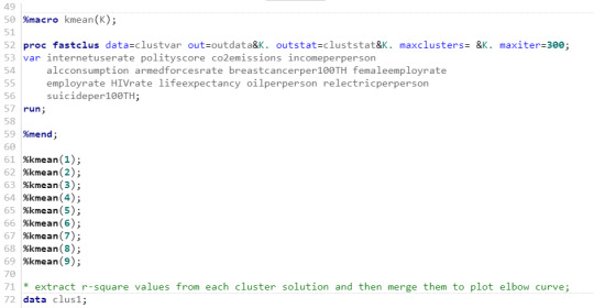
Running a k-means cluster analysis with the gapminder data set

First of all find below my syntax for the program:

Find my output here:

And my summary:

A k-means cluster analysis was conducted to identify underlying subgroups of indicators measuring social, economic and environmental statsitics based on their similarity on 13 variables that represent characteristics that could have an impact on internet use rate. Clustering variables included only quantitative variables being polity score, cumulative CO2 emission, income per person, alcohol consumption per adult (age +15), armed forces rate, breast cancer new cases per 100,000 female residents, female employ rate (female employees age +15), employ rate (total employees age +15), HIV rate (ages 15-49), life expectancy at birth (years), oil consumption per capita (tonnes per year and person), residential electricity consumption per person (kWh), suicide rate age adjusted per 100,000 and urban rate. All clustering variables were standardized to have a mean of 0 and a standard deviation of 1.

 Data were randomly split into a training set that included 70% of the observations (N=25) and a test set that included 30% of the observations (N=11). A series of k-means cluster analyses were conducted on the training data specifying k=1-9 clusters, using Euclidean distance. The variance in the clustering variables that was accounted for by the clusters (r-square) was plotted for each of the nine cluster solutions in an elbow curve to provide guidance for choosing the number of clusters to interpret.

 Figure 1. Elbow curve of r-square values for the nine cluster solutions

The elbow curve was inconclusive, suggesting that the 2, 3, 4, 7 and 8-cluster solutions might be interpreted. The results below are for an interpretation of the 4-cluster solution.

 Canonical discriminant analyses was used to reduce the 13 clustering variable down a few variables that accounted for most of the variance in the clustering variables. A scatterplot of the first two canonical variables by cluster (Figure 2 shown below) indicated that the observations in clusters 3 and 4 were densely packed with relatively low within cluster variance, and did not overlap with the other clusters. Cluster 2 was generally distinct, but the observations had greater spread suggesting higher within cluster variance. Observations in cluster 1 were spread out more than the other clusters, showing high within cluster variance. The results of this plot suggest that the best cluster solution may have fewer than 4 clusters, so it will be especially important to also evaluate the cluster solutions with fewer than 4 clusters.

 Figure 2. Plot of the first two canonical variables for the clustering variables by cluster.

The means on the clustering variables showed that, compared to the other clusters, indicators in cluster 3 had moderate levels on the clustering variables. They had a relatively low probability of employ rate (total employee age +15, but moderate levels of HIV rate (ages 15-49) and suicide rate age adjusted per 100,000. They also appeared to have fairly low levels of female employ rate (female employees age +15), armed forces rate, oil consumption per capita (tonnes per year and person) and breast cancer new cases per 100,000 female residents. With the exception of polity score, income per person, breast cancer new cases per 100,000 female residents, oil consumption per capita (tonnes per year and person, electricity consumption per person (kWh) and HIV rate (ages 15-49) cluster 2 had higher levels on the clustering variables compared to cluster 3, but moderate compared to clusters 1 and 4. On the other hand, cluster 4 included the most significant indicators. Indicators in cluster four had the highest likelihood of having a high alcohol consumption per adult (age +15), a very high likelihood of having a high oil consumption per capita (tonnes per year and person), more life expectancy at birth (years) and more oil consumption per capita (tonnes per year and person) compared to the other clusters. Cluster 2 appeared to include the least significant indicators. Compared to indicators in the other clusters, they were least likely to have a high polity score, and had the lowest CO2 emission, and armed and forces rate. They also had the lowest levels of female employ rate (female employees age +15), and lower employ rate (total employees age +15) and lower life expectancy at birth (years).

 In order to externally validate the clusters, an Analysis of Variance (ANOVA) was conducting to test for significant differences between the clusters on internet use rate. A tukey test was used for post hoc comparisons between the clusters. Results indicated significant differences between the clusters on internet use rate (F(3, 131)=111.07, p<.0001). The tukey post hoc comparisons showed significant differences between clusters on internet use rate, with the exception that clusters 1 and 4 were not significantly different from each other. Indicators in cluster 3 had the highest internet use rate (mean=19.63.99, sd=13.99), and cluster 2 had the lowest internet use rate (mean=8.79, sd=8.68).

[nicoerd-blog]

My Lasso Regression Project with the gapminder dataset

A lasso regression analysis was conducted to identify a subset of variables from a pool of 13 quantitative predictor variables that best predicted a quantitative response variable measuring the internet use rate. Quantitative predictor variables include polity score, cumulative CO2 emission, income per person, alcohol consumption per adult (age +15), armed forces rate, breast cancer new cases per 100,000 female residents, female employ rate (female employees age +15), employ rate (total employees age +15), HIV rate (ages 15-49), life expectancy at birth (years), oil consumption per capita (tonnes per year and person), residential electricity consumption per person (kWh), suicide rate age adjusted per 100,000 and urban rate. All predictor variables were standardized to have a mean of zero and a standard deviation of one.

Data were randomly split into a training set that included 70% of the observations (N= 40) and a test set that included 30% of the observations (N= 16 ). The least angle regression algorithm with k=10 fold cross validation was used to estimate the lasso regression model in the training set, and the model was validated using the test set. The change in the cross validation average (mean) squared error at each step was used to identify the best subset of predictor variables.

Figure 1. Change in the validation mean square error at each step

Of the 13 predictor variables, 4 were retained in the selected model. During the estimation process, income per person and life expectancy at birth (years) were most strongly associated with internet use rate, followed by breast cancer new cases per 100,000 female residents and alcohol consumption per adult (age +15). All aforementioned varibles were positively associated with internet use rate. These 4 variables accounted for 81.8% of the variance in the internet use rate response variable.

My code for the lasso regression:

[nicoerd-blog]

My gapminder research program using random forest

Random forest analysis was performed to evaluate the importance of a series of explanatory variables in predicting a binary, categorical response variable. The following quantitative explanatory variables were included as possible contributors to a random forest evaluating internet use rate (my response variable), polity score, cumulative CO2 emission, income per person, alcohol consumption per adult (age +15), armed forces rate, breast cancer new cases per 100,000 female residents, female employ rate (female employees age +15), employ rate (total employees age +15), HIV rate (ages 15-49), life expectancy at birth (years), oil consumption per capita (tonnes per year and person), residential electricity consumption per person (kWh), suicide rate age adjusted per 100,000 and urban rate. As all variables in the gapminder dataset are quantitative I split internet use rate into two categories, zero for rates lower than 50 and one for rates larger or equal than 50.

 The explanatory variables with the highest relative importance scores were income per person, residential electricity per person (kWh), life expectancy at birth (years) and breast cancer new cases per 100, 000 female residents. The accuracy of the random forest was 73.7%, with the subsequent growing of multiple trees rather than a single tree, adding little to the overall accuracy of the model and suggesting that interpretation of a single decision tree may be appropriate.

 My code:

My output:

[nicoerd-blog]

Running a classification tree for the gapminder dataset

Here is my final tree:

Decision tree analysis was performed to test nonlinear relationships among a series of explanatory variables and a binary, categorical response variable. As the gapminder dataset contains only quantitative varibles all cut points (quantitative) are tested. For the present analyses, the entropy “goodness of split” criterion was used to grow the tree and a cost complexity algorithm was used for pruning the full tree into a final subtree.

The following explanatory variables were included as possible contributors to a classification tree model evaluating internet use rate (my response variable), polity score, cumulative CO2 emission, income per person, alcohol consumption per adult (age +15), armed forces rate, breast cancer new cases per 100,000 female residents, female employ rate (female employees age +15), employ rate (total employees age +15), HIV rate (ages 15-49), life expectancy at birth (years), oil consumption per capita (tonnes per year and person), residential electricity consumption per person (kWh), suicide rate age adjusted per 100,000 and urban rate.

The deviance score was the first variable to separate the sample into two subgroups. People with a deviance income per person rate greater than 4893.635 were more likely to have used the internet regularly compared to people not meeting this cutoff.

Of the people with deviance income per person rate greater than or equal to 4893.635, a further subdivision was made with the dichotomous variable of residential electricity consumption per person (kWh). People who reported having a deviance residential electricity consumption per person rate greater than or equal to 583.596 were more likely to have used the internet regularly. People with a deviance score less than 583.596 who had a lower residential electricity consumption per person (kWh) were less likely to use the internet frequently. 

Of the people with deviance residential electricity per person (kWh) rate greater than or equal to 583.596, a further subdivision was made with the dichotomous variable of suicide rate age adjusted per 100,000. People who reported having a deviance suicide rate age adjusted per 100,000 greater than or equal to 7.773 were more likely to have used the internet regularly. People with a deviance rate less than 7.773 who had a lower suicide rate age adjusted per 100,000 were less likely to use the internet frequently.

The total model classified 100% of the sample correctly.

[nicoerd-blog]

Running a classification tree for the gapminder dataset

Here is my final tree:

Decision tree analysis was performed to test nonlinear relationships among a series of explanatory variables and a binary, categorical response variable. As the gapminder dataset contains only quantitative varibles all cut points (quantitative) are tested. For the present analyses, the entropy “goodness of split” criterion was used to grow the tree and a cost complexity algorithm was used for pruning the full tree into a final subtree.

The following explanatory variables were included as possible contributors to a classification tree model evaluating internet use rate (my response variable), polity score, cumulative CO2 emission, income per person, alcohol consumption per adult (age +15), armed forces rate, breast cancer new cases per 100,000 female residents, female employ rate (female employees age +15), employ rate (total employees age +15), HIV rate (ages 15-49), life expectancy at birth (years), oil consumption per capita (tonnes per year and person), residential electricity consumption per person (kWh), suicide rate age adjusted per 100,000 and urban rate.

The deviance score was the first variable to separate the sample into two subgroups. People with a deviance income per person rate greater than 4893.635 were more likely to have used the internet regularly compared to people not meeting this cutoff.

Of the people with deviance income per person rate greater than or equal to 4893.635, a further subdivision was made with the dichotomous variable of residential electricity consumption per person (kWh). People who reported having a deviance residential electricity consumption per person rate greater than or equal to 583.596 were more likely to have used the internet regularly. People with a deviance score less than 583.596 who had a lower residential electricity consumption per person (kWh) were less likely to use the internet frequently. 

Of the people with deviance residential electricity per person (kWh) rate greater than or equal to 583.596, a further subdivision was made with the dichotomous variable of suicide rate age adjusted per 100,000. People who reported having a deviance suicide rate age adjusted per 100,000 greater than or equal to 7.773 were more likely to have used the internet regularly. People with a deviance rate less than 7.773 who had a lower suicide rate age adjusted per 100,000 were less likely to use the internet frequently.

The total model classified 100% of the sample correctly.

My code:

[nicoerd-blog]

My logistic regression output

[nicoerd-blog]

Did another lurking variable confound the association between my original variables?

Yes, this is clearly the case. Income per person has an important impact on internet use rates and makes electricity per person not siginifcant any more. Interestingly the analysis revealed that having an internet use rate of 50 to 100 is indpendent of the income per person which emphasizes the importance that the internet has in our daily life irrespective of income.

[nicoerd-blog]

Did the results support my hypothesis?

My alternative hypothesis was that there is an association between electricity per person and internet use rate. That is true as long as I add no further lurking variables. However, as soon as I add income per person I cannot reject the hypothesis that there is no association. Income per person seems to have a greater impact on internet use rates.

[nicoerd-blog]

My summary

For my research I selected the internet use rate (2010 internet user (per 100 people)) as the response variable. I splitted this varible to get a binary variable so I can test a logistic regression model. Here I chose “0″ for rates from 0 to 50 and “1″ for rates from 50 to 100. I also tested several explanatory variables, namely polityscore (2009 democracy score (Polity)) that I splitted into two categories as well for better visualization, “0″ vor negative scores -10 to - 1 (less democratic), and “1″ for positive scores 0 to 10 (more democratic)), income per person  (2010 Gross Domestic Product per capita in constant 2000 US$),  urbanrate (2008 urban population (% of total)) and electricity per person (2008 residential electricity consumption, per person (kwh)). All these variables are centered quantitative explanatory variables. First I created a linear regression to test which explanatory variables contribute most to the response variable internet use rate:

This result shows clearly that only the intercept (p = 0.0016), the electricity per person (p = 0.0138) and income per person (p < 0.0001) contribute significantly to the response variable internet use rate.

In the second step I created a Logistic Regression model. I used the electricity per person  as it is significant in the Linear regression model. My hypothesis is that available electricity per person has an impact on the internet use rate.

As you can see this is true. Both the intercept with pr > ChiSq = 0.0072 and the electricity per person with Pr > ChiSq < 0.0001  are signicant. The odds ratio is 1.001 which lies in the condidence interval 1.001 to 1.002. This means that the odds of having an internet use rate from 50 to 100 is more than one time higher for those with higher electricity rates per person than those with lower electricity rates per person.

In the next step I add income per person as the second explanatory variable in the logistic regression model to get the following output:

Here we can see that income per person has a significant impact on the internet use rate and confounds the association between electricity per person and internet use rate. After controlling for electricity per person income per person is significant with Pr > ChiSq = 0.0007 and the odds ratio of 1 lies between the confidence interval 1 to 1.001. This means that the odds of having an internet use rate from 50 to 100 is equally likely for those with lower income than those with higer income per person. However electricity per person is not significant any more. After controlling for income per person Pr > ChiSq = 0.5179. So we must rule out electricity per person for the odds ratio analysis and conclude that there is no association with the internet use ratio after controlling for income per person.

[nicoerd-blog]

My multiple regression output

[nicoerd-blog]

Analysis of regression diagnostic plots

Here are both non standardized and standardized residual plots:

Especially in the standardized plot 5 observation of the distribution of residuals are significant outliers because they are not within 2 stand deviations or 60% around the mean. This might give some evidence that the normality and independency assumption which is essential for regerssion analysis might by violated. Another prove for the presence of additional lurking variables not included in the model.

 Here is the leverage plot:

The leverage plot also confirms some trouble with the data. We have 4 outliers that fortunately have only a small leverage effect on the regession association. However, which is worrying, there is one outlier in the data that has a huge lever.

Now the qq-plot:

This plot further confirm the presence of non-normality as the plots follow the straight line only between the -1 and +1 quantiles.

And the partial plots:

The partial plots show that the urbanrate has partial residual with few outliers with a quite good line fit. Even the outliers in this regression follow the straight line and are only outliers in magnitude of the regressor residual. A similar but weaker model fit can also be seen for intercept and polity score squared. Polity score however has a very bad model fit with many partial residual outliers and clustering of partial residuals in the higher magnitude region of the partial regressor residual.

[nicoerd-blog]

Was there a confounding effect?

There was a clear confounding effect. Urban rate has a significantly higher explanatory power than polity score with regard to the internet use rate. The effect was so large that is might be wise to consider other lurking variables than urban rate that might have a significant effect on the internet use rate as well. 

[nicoerd-blog]

My report after the results

My hypothesis was that the polity score has an impact on the internetuserate. However after controlling for urban rate we see that this effect is not significant any more. Due to the fact I cannot statistically prove an association between my primary explanatory variable and my response variable my hypothesis cannot be supported.

[nicoerd-blog]

My findings for my gapminder research project

My project is about exmining the association between polity score (quantitative explanatory variable) and internet use rate (quantitative response variable) if there is another variable urban rate (quantitive explanatory varible) that might confound the association between the two original variables.

Firstly we see there is no linear relationship between polity score and internet use rate as tje linear regression results show only a weak positive linear association and the polynomial regression results show a u-shaped association :

This means that the internet use rate is high for autocracies as well as for democracies however for anocracies with a score close to 0 the internet use rate is quite low.

Now let’s introduce a third variable internet use rate. As both polity score and urban rate are quantitative variables I need to center their means for the purpose of this research to created 2 new centered variables urbanrate_c and polityscore_c:

Both means now have very small values close to zero which confirms succesful centering.

Now I look at the linear association between polity score and internet use rate. I completely rule out the effect of the urbanrate:

Here we see that the intercept beta0 of 32.53 is highly significant with p<.0001 as is the regeression coefficient beta1 of 1.6 with p<.0001. In addition both regression parameters do not contain a zero value when tested ate the 5% significance level. So we can reject the assumption of no dependency under those circumstances. However, only 13.28% of the variation in the internet use rate are explained by the polity score.

Let’s have a look at the association between our third variable urban rate and internet use rate. This time we leave out polity score:

Here we see that the intercept beta0 of 32.53 is highly significant with p<.0001 as is the regeression coefficient beta1 of 0.81 with p<.0001. In addition both regression parameters do not contain a zero value when tested ate the 5% significance level. So we can reject the assumption of no dependency under those circumstances. Here 44.7% of the variation in the internet use rate are explained by the urban rate. That is quite a lot!

Lastly, let’s have a look at what happens if we take into account both explanatory variables polity score and urban rate and discuss a multiple regression output:

Here we see that the intercept beta0 of 13.03 is highly significant with p<.0001 as is the regeression coefficient beta1 of 0.35 with p<.0001 of the squared polityscore term and the regression coefficient beta1 of 0.57 with p<.0001 of the urbanrate. In addition all those regression parameters do not contain a zero value when tested ate the 5% significance level. So we can reject here the assumption of no dependency. However when incorporating the effect of urban rate the polity score with a beta1 of 0.25 is not significant any more with p=0.3335 which is greater than 0.05 and the 95% confidence level now contains 0. So after controlling for urban rate we cannot reject our independency assumption for the association between polity score and internet use rate. Here 62.65% of the variation in the internet use rate are explained by the urban rate. That is even more!