#(I can also give the raw data and/or python code | Explore Tumblr posts and blogs

hydrus · 5 years ago

Text

Version 422

youtube

windows

zip

exe

macOS

app

linux

tar.gz

🎉🎉 It was hydrus's birthday this week! 🎉🎉

I had a great week. I mostly fixed bugs and improved quality of life.

tags

It looks like when I optimised tag autocomplete around v419, I accidentally broke the advanced 'character:*'-style lookups (which you can enable under tags->manage tag display and search. I regret this is not the first time these clever queries have been broken by accident. I have fixed them this week and added several sets of unit tests to ensure I do not repeat this mistake.

These expansive searches should also work faster, cancel faster, and there are a few new neat cache optimisations to check when an expensive search's results for 'char' or 'character:' can quickly provide results for a later 'character:samus'. Overall, these queries should be a bit better all around. Let me know if you have any more trouble.

The single-tag right-click menu now always shows sibling and parent data, and for all services. Each service stacks siblings/parents into tall submenus, but the tall menu feels better to me than nested, so we'll see how that works out IRL. You can click any sibling or parent to copy to clipboard, so I have retired the 'copy' menu's older and simpler 'siblings' submenu.

misc

Some websites have a 'redirect' optimisation where if a gallery page has only one file, it moves you straight to the post page for that file. This has been a problem for hydrus for some time, and particularly affected users who were doing md5: queries on certain sites, but I believe the downloader engine can now handle it correctly, forwarding the redirect URL to the file queue. This is working on some slightly shakey tech that I want to improve more in future, but let me know how you get on with it.

The UPnPc executables (miniupnp, here https://miniupnp.tuxfamily.org/) are no longer bundled in the 'bin' directory. These files were a common cause of anti-virus false positives every few months, and are only used by a few advanced users to set up servers and hit network->data->manage upnp, so I have decided that new users will have to install it themselves going forward. Trying to perform a UPnP operation when the exe cannot be found now gives a popup message talking about the situation and pointing to the new readme in the bin directory.

After working with a user, it seems that some clients may not have certain indices that speed up sibling and parent lookups. I am not totally sure if this was due to hard drive damage or broken update logic, but the database now looks for and heals this problem on every boot.

parsing (advanced)

String converters can now encode or decode by 'unicode escape characters' ('\u0394'-to-'Δ') and 'html entities' ('&'-to-'&'). Also, when you tell a json formula to fetch 'json' rather than 'string', it no longer escapes unicode.

The hydrus downloader system no longer needs the borked 'bytes' decode for a 'file hash' content parser! These content parsers now have a 'hex'/'base64' dropdown in their UI, and you just deliver that string. This ugly situation was a legacy artifact of python2, now finally cleared up. Existing string converters now treat 'hex' or 'base64' decode steps as a no-op, and existing 'file hash' content parsers should update correctly to 'hex' or 'base64' based on what their string converters were doing previously. The help is updated to reflect this. hex/base64 encodes are still in as they are used for file lookup script hash initialisation, but they will likely get similar treatment in future.

birthday

🎉🎉🎉🎉🎉

On December 14th, 2011, the first non-experimental beta of hydrus was released. This week marks nine years. It has been a lot of work and a lot of fun.

Looking back on 2020, we converted a regularly buggy and crashy new Qt build to something much faster and nicer than we ever had with wx. Along with that came mpv and smooth video and finally audio playing out of the client. The PTR grew to a billion mappings(!), and with that came many rounds of database optimisation, speeding up many complicated tag and file searches. You can now save and load those searches, and most recently, search predicates are now editable in-place. Siblings and parents were updated to completely undoable virtual systems, resulting in much faster boot time and thumbnail load and greatly improved tag relationship logic. Subscriptions were broken into smaller objects, meaning they load and edit much faster, and several CPU-heavy routines no longer interrupt or judder browsing. And the Client API expanded to allow browsing applications and easier login solutions for difficult sites.

There are still a couple thousand things I would like to do, so I hope to keep going into 2021. I deeply appreciate the feedback, help, and support over the years. Thank you!

If you would like to further support my work and are in a position to do so, my simple no-reward Patreon is here: https://www.patreon.com/hydrus_dev

full list

advanced tags:

fixed the search code for various 'total' autocomplete searches like '*' and 'namespace:*', which were broken around v419's optimised regular tag lookups. these search types also have a round of their own search optimisations and improved cancel latency. I am sorry for the trouble here

expanded the database autocomplete fetch unit tests to handle these total lookups so I do not accidentally kill them due to typo/ignorance again

updated the autocomplete result cache object to consult a search's advanced search options (as under _tags->manage tag display and search_) to test whether a search cache for 'char' or 'character:' is able to serve results for a later 'character:samus' input

optimised file and tag search code for cases where someone might somehow sneak an unoptimised raw '*:subtag' or 'namespace:*' search text in

updated and expanded the autocomplete result cache unit tests to handle the new tested options and the various 'total' tests, so they aren't disabled by accident again

cancelling a autocomplete query with a gigantic number of results should now cancel much quicker when you have a lot of siblings

the single-tag right-click menu now shows siblings and parents info for every service, and will work on taglists in the 'all known tags' domain. clicking on any item will copy it to clipboard. this might result in megatall submenus, but we'll see. tall seems easier to use than nested per-service for now

the more primitive 'siblings' submenu on the taglist 'copy' right-click menu is now removed

right-click should no longer raise an error on esoteric taglists (such as tag filters and namespace colours). you might get some funky copy strings, which is sort of fun too

the copy string for the special namespace predicate ('namespace:*anything*') is now 'namespace:*', making it easier to copy/paste this across pages

misc:

the thumbnail right-click 'copy/open known urls by url class' commands now exclude those urls that match a more specific url class (e.g. /post/123456 vs /post/123456/image.jpg)

miniupnpc is no longer bundled in the official builds. this executable is only used by a few advanced users and was a regular cause of anti-virus false positives, so I have decided new users will have to install it manually going forward.

the client now looks for miniupnpc in more places, including the system path. when missing, its error popups have better explanation, pointing users to a new readme in the bin directory

UPnP errors now have more explanation for 'No IGD UPnP Device' errortext

the database's boot-repair function now ensures indices are created for: non-sha256 hashes, sibling and parent lookups, storage tag cache, and display tag cache. some users may be missing indices here for unknown update logic or hard drive damage reasons, and this should speed them right back up. the boot-repair function now broadcasts 'checking database for faults' to the splash, which you will see if it needs some time to work

the duplicates page once again correctly updates the potential pairs count in the 'filter' tab when potential search finishes or filtering finishes

added the --boot_debug launch switch, which for now prints additional splash screen texts to the log

the global pixmaps object is no longer initialised in client model boot, but now on first request

fixed type of --db_synchronous_override launch parameter, which was throwing type errors

updated the client file readwrite lock logic and brushed up its unit tests

improved the error when the client database is asked for the id of an invalid tag that collapses to zero characters

the qss stylesheet directory is now mapped to the static dir in a way that will follow static directory redirects

downloaders and parsing (advanced):

started on better network redirection tech. if a post or gallery URL is 3XX redirected, hydrus now recognises this, and if the redirected url is the same type and parseable, the new url and parser are swapped in. if a gallery url is redirected to a non-gallery url, it will create a new file import object for that URL and say so in its gallery log note. this tentatively solves the 'booru redirects one-file gallery pages to post url' problem, but the whole thing is held together by prayer. I now have a plan to rejigger my pipelines to deal with this situation better, ultimately I will likely expose and log all redirects so we can always see better what is going on behind the scenes

added 'unicode escape characters' and 'html entities' string converter encode/decode types. the former does '\u0394'-to-'Δ', and the latter does '&'-to-'&'

improved my string converter unit tests and added the above to them

in the parsing system, decoding from 'hex' or 'base64' is no longer needed for a 'file hash' content type. these string conversions are now no-ops and can be deleted. they converted to a non-string type, an artifact of the old way python 2 used to handle unicode, and were a sore thumb for a long time in the python 3 parsing system. 'file hash' content types now have a 'hex'/'base64' dropdown, and do decoding to raw bytes at a layer above string parsing. on update, existing file hash content parsers will default to hex and attempt to figure out if they were a base64 (however if the hex fails, base64 will be attempted as well anyway, so it is not critically important here if this update detection is imperfect). the 'hex' and 'base64' _encode_ types remain as they are still used in file lookup script hash initialisation, but they will likely be replaced similarly in future. hex or base64 conversion will return in a purely string-based form as technically needed in future

updated the make-a-downloader help and some screenshots regarding the new hash decoding

when the json parsing formula is told to get the 'json' of a parsed node, this no longer encodes unicode with escape characters (\u0394 etc...)

duplicating or importing nested gallery url generators now refreshes all internal reference ids, which should reduce the liklihood of accidentally linking with related but differently named existing GUGs

importing GUGs or NGUGs through Lain easy import does the same, ensuring the new objects 'seem' fresh to a client and should not incorrectly link up with renamed versions of related NGUGs or GUGs

added unit tests for hex and base64 string converter encoding

next week

Last week of the year. I could not find time to do the network updates I wanted to this week, so that would be nice. Otherwise I will try and clean and fix little things before my week off over Christmas. The 'big thing to work on next' poll will go up next week with the 423 release posts.

#release

1 note · View note

greenplumbboblover · 8 months ago

Text

THIS ISSUE HAS BEEN RESOLVED!

(Source: https://modthesims.info/showthread.php?t=687747 )

TL;DR: What happened?

Two creators had unfortunately been victim to their passwords being leaked. The people who are behind these types of TS4 malware issues tend to find leaked passwords and then sharing their Trojan file.

IF you downloaded any of these 4 items in the last 24 hours: 1. No Mosaic / Censor Mod for The Sims 4 - Toddler Compatibility Update! 2. AllCheats - Get your cheats back! 3. CAS FullEditMode Always On (Updated 6/26/18) 4. Full House Mod - Increase your Household Size! [Still Compatible as of 1/25/18] Just know that they were only live for 1,5 hours. The chances that you downloaded something malware are quite low due to this. However, just to be safe, it's good to delete them anyways if you did download them 24 hours before as of this reblog post.

So: Just a reminder to, well, everyone using the internet: Make sure to change your passwords periodically! (and, if possible, use an authentication app).

As far as I know, MTS is working on making it much harder to update posts when you've been inactive for a while! So in the future, the hackers would need access to your email provider to include malware in your mods. I believe this code is already live as we speak.

How to stay safe downloading anything CC related in the future:

Know that this issue is seemingly a big issue in The sims 4 community! While the other communities are certainly not ruled out to be able to have malware in them, it seems this group of hackers are really focused on The Sims 4 community as a whole.

What files are the issue?

ts4script files. Because it's raw python AND TS4 doesn't have great restrictions for script mods in place, these people can modify the python file to create a .dll file on running the game. That's how they get information if they're lucky.

.exe files or files that look like another file type but are an .exe file. (or some executable file like a bash script, etc). MTS does check these things before approving, but do be careful when downloading these things from tumblr or github. Make sure to check the comments there instead.

What files CANNOT ever get malware in them?

Simply said: .Package files. Exception for maybe the .package files that are actually ts4script files, but that's really from the ancient TS4 days.

With other words, your: CasParts, Lots, Cosmetics, Hair, Sims, Recolours, Objects CANNOT have malware in them

The only "kind of" malware we saw back in the days in Package files was the infamous TS3 Doll corruption bug. But that didn't collect your data, just corrupted your save/game 😉

What ways can I detect if something is malware at first sight?

99% of script modders, when updating their mods, WILL add WHY they updated their mod in the first place. If you do NOT see any update reasons in the description, it's probably malware.

Check the comments! If you're not sure, always check if someone left a comment (or in Tumblr's case, a Reblog).

Trust your gut feeling! Does something seem strange? A bit out of place from the usual? Give it a few days before you download the mod.

Package files SHOULD NEVER have a way of "installing your content" through an .exe file "For simplicity", because 99% of the cases, it's malware to trick you. Unless there is a excellent reason for it (and I mean REALLY good reason).

More or less a download site related thing: If a download site has a billion buttons saying "Download". Please don't press these. They are most likely Malware too, but definitely shady ads. For those pages, it would be best to leave the item alone, unless you really know what you're doing!

Conclusion

While these discord server announcements mean well, it frustrates me to see that they mention that EVERYTHING is compromised. Whereas in reality it's only TS4Scripts and .exe files that can do harm.

I know they mean well! And wanting to protect people! But at the same time, it also spreads a sense of misinformation that can harm creators, websites, you name it.

So, instead, I would love to advise them to educate their members instead on what files can be the problem! And how to detect them. The more we get this into the world, the better we will be able to protect one another from downloading bad things!

And of course, websites that share CC, should make an effort to prevent this in the future. I'm happy MTS is doing this at the moment.

Stay safe!

(Sourced from the Sims After Dark discord server)

DO NOT DOWNLOAD ANY MODS FROM MODTHESIMS! Numerous mods there (including those by TwistedMexi) are being compromised by hackers adding a malicious file with the mods

Please reblog!!

#Signal boost #please reblog #the sims 4 #ts3 #ts4 #sims 4 #mod the sims #sims 4 community #sims community #sims 2 community #ts2 community #ts4 community #the sims 2 #ts2 #sims 2 #mts

4K notes · View notes

azaleakamellia · 5 years ago

Text

zero to pandas

There are alot of Python courses out there that we can jump into and get started with. But to a certain extent in that attempt to learn the language, the process becomes unbearably long and frustratingly slow. We all know the feeling of wanting to run before we could learn how to walk; we really wanna get started with some subtantial project but we do not know enough to even call the data into the terminal for viewing.

Back in August, freeCodeCamp in collaboration with Jovian.ai, organized a very interesting 6-week MOOC called Data Analysis with Python: Zero to Pandas and as a self-proclaimed Python groupie, I pledged my allegiance!

If there are any expectation that I've managed to whizz myself through the course and obtained a certificate, nothing of that sort happened; I missed the deadline cause I was busy testing out every single code I found and work had my brain on overdrive. I can't...I just...can't. Even with the extension, I was short of 2 Pythonic answers required to earn the certificate. But don't mistake my blunders for the quality of the content this course has to offer; is worth every gratitude of its graduates!

Zero to Pandas MOOC is a course that spans over 6 weeks with one lecture webinar per week that compacts the basics of Python modules that are relevant in executing data analysis. Like the play on its name, this course assumes no prior knowledge in Python language and aims to teach prospective students the basics on Python language structure AND the steps in analyzing real data. The course does not pretend that data analytics is easy and cut-corners to simplify anything. It is a very 'honest' demonstration that effectively gives overly ambitious future data analysts a flick on the forehead about data analysis. Who are we kidding? Data analysis using programming language requires sturdy knowledge in some nifty codes clean, splice and feature engineer the raw data and real critical thinking on figuring out 'Pythonic' ways to answer analytical questions. What does it even mean by Pythonic ways? Please refer to this article by Robert Clark, How to be Pythonic and Why You Should Care. We can discuss it somewhere down the line, when I am more experienced to understand it better. But for now, Packt Hub has the more comprehensive simple answer; it simply is an adjective coined to describe a way/code/structure of a code that utilizes or take advantage of the Python idioms well and displays the natural fluency in the language.

The bottom line is, we want to be able to fully utilize Python in its context and using its idioms to analyze data.

The course is conducted at Jovian.ai platform by its founder; Aakash and it takes advantage of Jupyter-like notebook format; Binder, in addition to making the synchronization available at Kaggle and Google's Colab. Each webinar in this course spans over close to 2 hours and each week, there are assignments on the lecture given. The assignments are due in a week but given the very disproportionate ratio of students and instructors, there were some extensions on the submission dates that I truly was grateful for. Forum for students is available at Jovian to engage students into discussing their ideas and question and the teaching body also conducts office hours where students can actively ask questions.

The instructor's method of teaching is something I believe to be effective for technical learners. In each lectures, he will be teaching the codes and module requires to execute certain tasks in the thorough procedure of the data analysis task itself. From importing the .csv formatted data into Python to establishing navigation to the data repository...from explaining what the hell loops are to touching base with creating functions. All in the controlled context of two most important module for the real objective of this course; Numpy and Pandas.

My gain from this course is immensely vast and that's why I truly think that freeCodeCamp and Jovian.ai really put the word 'tea' to 'teachers'. Taking advantage of the fact that people are involuntarily quarantined in their house, this course is something that should not be placed aside in the 'LATER' basket. I managed to clear my head to understand what 'loop' is! So I do think it can solve the world's problem!

In conclusion, this is the best course I have ever completed (90%!) on data analysis using Python. I look forward to attending it again and really finish up that last coursework.

Oh. Did I not mention why I got stuck? It was the last coursework. We are required to demonstrate all the steps of data analysis on data of our choice, create 5 questions and answer them using what we've learned throughout the course. Easy eh? Well, I've always had the tendency of digging my own grave everytime I get awesome cool assignments. But I'm not saying I did not do it :). Have a look-see at this notebook and consider the possibilities you can grasp after you've completed the course. And that's just my work...I'm a standard C-grade student.

And the exciting latest news from Jovian.ai is that they have upcoming course at Jovian for Deep Learning called Deep Learning with PyTorch: Zero to GANS! That's actually yesterday's news since they organized it earlier this year...so yeah...this is an impending second cohort! Tentatively, the course will start on Nov 14th. Click the link below to sign-up and get ready to attack the nitty-gritty. Don't say I didn't warn ya.

And that's me, reporting live from the confinement of COVID pandemic somewhere in a developing country at Southeast Asia....

#studyblr #data science #python #mooc

1 note · View note

anubhavanand12qw · 5 years ago

Text

DTC Prediction & Analysis

Data from the vehicle can be very useful for predicting faults and errors in the vehicle, but most of the data which comes from the sensors is redundant data. In this paper Diagnostic Trouble Code (DTC) in a vehicle is being predicted along with, eliminating the issue of redundant data.

The data used in my project was from Eicher's heavy-duty trucks. Some of them have sensors installed in them, which sends a combination of vehicle sensor data and vehicle data. Before feeding this data to Deep Neural Network (DNN), data is divided into multiple clusters based on the requirement which will be discussed in a later section of this paper. These clusters are then pre-processed in-order to remove redundancy from the data, as much as possible. Once the dataset is clean and ready to use, the important features are extracted from the data to feed into the machine learning model.

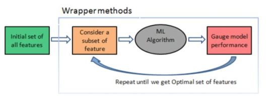
Feature extraction can be done using a method called wrapper method. Wrapper method is used to find out the number of minimum features that are most significant in predicting the output. The wrapper method takes all features as input parameters, a machine learning model for prediction, scoring technique (in this case r-square), and a significance level (default 0.05). For instance, if we are using a linear regression model, then it will calculate the p-value for each feature, which is also the null hypothesis. If we are using a backward elimination technique in the wrapper method, then it will eliminate a feature if its p-value is greater than the significance level.

Once we have all the required features, we applied 4 different models to predict the output. The models which we have used in this paper are Decision Tree, Random Forest Regressor, Logistic Regression, and Deep Neural Network. The reason behind using Decision Tree, Random Forest Regressor, and Logistic Regression along with DNN are, these models also work well on this kind of dataset and we can use it to compare results with each other.

The outcome of anything depends eventually upon the results which are generated from it. In this section, we will discuss the result for each phase of the project. Starting from data collection to model prediction. As each step is dependent on one another and gives crucial information about the data. But a certain part of each stage is independent of each other. Hence, it is important to know about the results of each stage. Starting from the data collection, we take raw data from the sensor and pre-process it in a way so that we can use it for DTC predicting and further use it for analysis of various other things as well. Therefore, the result of the initial part of the project is data, loaded with valuable information, which the organization can use as they want.

The next part was based on the prediction of DTC. As stated earlier that we used 4 different models and compared the output of each model with one another. Amongst which Deep Neural Network (DNN) was producing the best result. This is because DNN can easily identify patterns and meaningful information from the dataset if the data are sufficient.

Once the model has successfully started predicting DTCs, this information can be used in many places. For instance, if there is a critical error or fault which might occur in a vehicle, the driver can be alerted in advance. This way, any major damage to the vehicle can be avoided. Such prediction is very helpful and beneficial for the organization, customer, and the dealer.

This project has helped me in many ways. I got to learn a lot from it. Also, it provided me with a platform to test my skills in machine learning and data analytics. The main learning outcome of this project is listed below:

§ I got to learn about real-world data. How it is generated and transmitted from the vehicle to the server.

§ I learnt about the different models of vehicle and its parts.

§ Attain more clarity on data mining and data pre-processing.

§ Learnt about the different data and their relationship with each other.

§ Got a better understanding of machine learning models.

§ Learnt about the visualizing techniques in Python using Matplotlib.

§ Learnt, how to handle big data using python and techniques to work upon it.

§ Learnt more about Deep Neural Network (DNN) and its layers.

#bennett university #machine learning #Bennett University CSE Handle #Dr. Deepak Garg #Dr. Suneet Gupta #VE Commercial Vehicles Ltd.

1 note · View note

holytheoristtastemaker · 5 years ago

Quote

The coronavirus outbreak is taking over headlines. Due to the spread of COVID-19, remote work is suddenly an overnight requirement for many. You might be working from home as you are reading this article. With millions working from home for many weeks now, we should seize this opportunity to improve our skills in the domain we are focusing on. Here is my strategy to learn Data Science while working from home with few personal real life projects. "So what should we do?" "Where should we start learning?" Grab your coffee as I explain the process of how you can learn data science sitting at home. This blog is for everyone, from beginners to professionals. Photo by Nick Morrison on Unsplash Prerequisites To start this journey, you will need to cover the prerequisites. No matter which specific field you are in, you will need to learn the following prerequisites for data science. Logic/Algorithms: It’s important to know why we need a particular prerequisite before learning it. Algorithms are basically a set of instructions given to a computer to make it do a specific task. Machine learning is built from various complex algorithms. So you need to understand how algorithms and logic work on a basic level before jumping into complex algorithms needed for machine learning. If you are able to write the logic for any given puzzle with the proper steps, it will be easy for you to understand how these algorithms work and you can write one for yourself. Resources: Some awesome free resources to learn data structures and algorithms in depth. Statistics: Statistics is a collection of tools that you can use to get answers to important questions about data. Machine learning and statistics are two tightly related fields of study. So much so that statisticians refer to machine learning as “applied statistics” or “statistical learning”. Image source : http://me.me/ The following topics should be covered by aspiring data scientists before they start machine learning. Measures of Central Tendency — mean, median, mode, etc Measures of Variability — variance, standard deviation, z-score, etc Probability — probability density function, conditional probability, etc Accuracy — true positive, false positive, sensitivity, etc Hypothesis Testing and Statistical Significance — p-value, null hypothesis, etc Resources: Learn college level statistics in this free 8 hour course. Business: This depends on which domain you want to focus on. It basically involves understanding the particular domain and getting domain expertise before you get into a data science project. This is important as it helps in defining our problem accurately. Resources: Data science for business Brush up your basics This sounds pretty easy but we tend to forget some important basic concepts. It gets difficult to learn more complex concepts and the latest technologies in a specific domain without having a solid foundation in the basics. Here are few concepts you can start revising: Python programming language Python is widely used in data science. Check out this collection of great Python tutorials and these helpful code samples to get started. Image source : memecrunch.com You can also check out this Python3 Cheatsheet that will help you learn new syntax that was released in python3. It'll also help you brush up on basic syntax. And if you want a great free course, check out this Python for Everybody course from Dr. Chuck. General data science skills Want to take a great course on data science concepts? Here's a bunch of data science courses that you can take online, ranked according to thousands of data points. Resources: Data science for beginners - free 6 hour course, What languages should you learn for data science? Data Collection Now it is time for us to explore all the ways you can collect your data. You never know where your data might be hiding. Following are a few ways you can collect your data. Web scraping Web scraping helps you gather structured data from the web, select some of that data, and keep what you selected for whatever use you require. You can start learning BeautifulSoup4 which helps you scrape websites and make your own datasets. Advance Tip: You can automate browsers and get data from interactive web pages such as Firebase using Selenium. It is useful for automating web applications and automating boring web based administration Resources: Web Scraping 101 in Python Cloud servers If your data is stored on cloud servers such as S3, you might need to get familiar with how to get data from there. The following link will help you understand how to implement them using Amazon S3. Resources : Getting started with Amazon S3, How to deploy your site or app to AWS S3 with CloudFront APIs There are millions of websites that provide data through APIs such as Facebook, Twitter, etc. So it is important to learn how they are used and have a good idea on how they are implemented. Resources : What is an API? In English, please, How to build a JSON API with Python, and Getting started with Python API. Data Preprocessing This topic includes everything from data cleaning to feature engineering. It takes a lot of time and effort. So we need to dedicate a lot of time to actually learn it. Image source : https://www.pinterest.com/pin/293648838181843463/ Data cleaning involves different techniques based on the problem and data type. The data needs to be cleaned from irrelevant data, syntax erros, data inconsistencies and missing data. The following guide will get you started with data cleaning. Resources : Ultimate guide to data cleaning Data Preprocessing is an important step in which the data gets transformed, or encoded, so that the machine can easily parse it. It requires time as well as effort to preprocess different types of data which include numerical, textual and image data. Resources : Data Preprocessing: Concepts, All you need to know about text preprocessing for NLP and Machine Learning, Preprocessing for deep learning. Machine Learning Finally we reach our favourite part of data science: Machine Learning. Image source : https://in.pinterest.com/pin/536209899383255279/ My suggestion here would be to first brush up your basic algorithms. Classification — Logistic Regression, RandomForest, SVM, Naive Bayes, Decision Trees Resources : Types of classification algorithms in Machine Learning, Classification Algorithms in Machine Learning Regression — Linear Regression, RandomForest, Polynomial Regression Resources : Introduction to Linear Regression , Use Linear Regression models to predict quadratic, root, and polynomial functions, 7 Regression Techniques you should know, Selecting the best Machine Learning algorithm for your regression problem, Clustering — K-Means Clustering, DBSCAN, Agglomerative Hierarchical Clustering Resources : Clustering algorithms Gradient Boosting — XGBoost, Catboost, AdaBoost Resources : Gradient boosting from scratch, Understanding Gradient Boosting Machines I urge you all to understand the math behind these algorithms so you have a clear idea of how it actually works. You can refer to this blog where I have implemented XGBoost from scratch — Implementing XGBoost from scratch Now you can move on to Neural Networks and start your Deep Learning journey. Resources: Deep Learning for Developers, Introduction to Deep Learning with Tensorflow, How to develop neural networks with Tensorflow, Learn how deep neural networks work You can then further dive deep into how LSTM, Siamese Networks, CapsNet and BERT works. Hackathons: Image Source : https://me.me/ Now we need to implement these algorithms on a competitive level. You can start looking for online Data Science Hackathons. Here is the list of websites where I try to compete with other data scientists. Analytics Vidhya — https://datahack.analyticsvidhya.com/contest/all/ Kaggle — https://www.kaggle.com/competitions Hackerearth — https://www.hackerearth.com/challenges/ MachineHack — https://www.machinehack.com/ TechGig — https://www.techgig.com/challenge Dare2compete — https://dare2compete.com/e/competitions/latest Crowdanalytix — https://www.crowdanalytix.com/community To have a look at a winning solution, here is a link to my winning solution to one online Hackathon on Analytics Vidhya — https://github.com/Sid11/AnalyticsVidhya_DataSupremacy Projects: We see people working on dummy data and still don’t get the taste of how actual data looks like. In my opinion, working on real life data gives you a very clear idea how data in real life looks like. The amount of time and effort required in cleaning real life data takes about 70% of your project’s time. Here are the best free open data sources anyone can use Open Government Data — https://data.gov.in/ Data about real contributed by thousands of users and organizations across the world — https://data.world/datasets/real 19 public datasets for Data Science Project — https://www.springboard.com/blog/free-public-data-sets-data-science-project/ Business Intelligence After you get the results from your project, it is now time to make business decisions from those results. Business Intelligence is a suite of software and services that helps transform data into actionable intelligence and knowledge. This can be done by creating a dashboard from the output of our model. Tableau is a powerful and the fastest growing data visualization tool used in the Business Intelligence Industry. It helps in simplifying raw data into the very easily understandable format. Data analysis is very fast with Tableau and the visualizations created are in the form of dashboards and worksheets.

http://damianfallon.blogspot.com/2020/03/how-to-improve-your-data-science-skills_31.html

#SEO #Local SEO training

1 note · View note

srasamua · 6 years ago

Text

Using Python to recover SEO site traffic (Part three)

When you incorporate machine learning techniques to speed up SEO recovery, the results can be amazing.

This is the third and last installment from our series on using Python to speed SEO traffic recovery. In part one, I explained how our unique approach, that we call “winners vs losers” helps us quickly narrow down the pages losing traffic to find the main reason for the drop. In part two, we improved on our initial approach to manually group pages using regular expressions, which is very useful when you have sites with thousands or millions of pages, which is typically the case with ecommerce sites. In part three, we will learn something really exciting. We will learn to automatically group pages using machine learning.

As mentioned before, you can find the code used in part one, two and three in this Google Colab notebook.

Let’s get started.

URL matching vs content matching

When we grouped pages manually in part two, we benefited from the fact the URLs groups had clear patterns (collections, products, and the others) but it is often the case where there are no patterns in the URL. For example, Yahoo Stores’ sites use a flat URL structure with no directory paths. Our manual approach wouldn’t work in this case.

Fortunately, it is possible to group pages by their contents because most page templates have different content structures. They serve different user needs, so that needs to be the case.

How can we organize pages by their content? We can use DOM element selectors for this. We will specifically use XPaths.

For example, I can use the presence of a big product image to know the page is a product detail page. I can grab the product image address in the document (its XPath) by right-clicking on it in Chrome and choosing “Inspect,” then right-clicking to copy the XPath.

We can identify other page groups by finding page elements that are unique to them. However, note that while this would allow us to group Yahoo Store-type sites, it would still be a manual process to create the groups.

A scientist’s bottom-up approach

In order to group pages automatically, we need to use a statistical approach. In other words, we need to find patterns in the data that we can use to cluster similar pages together because they share similar statistics. This is a perfect problem for machine learning algorithms.

BloomReach, a digital experience platform vendor, shared their machine learning solution to this problem. To summarize it, they first manually selected cleaned features from the HTML tags like class IDs, CSS style sheet names, and the others. Then, they automatically grouped pages based on the presence and variability of these features. In their tests, they achieved around 90% accuracy, which is pretty good.

When you give problems like this to scientists and engineers with no domain expertise, they will generally come up with complicated, bottom-up solutions. The scientist will say, “Here is the data I have, let me try different computer science ideas I know until I find a good solution.”

One of the reasons I advocate practitioners learn programming is that you can start solving problems using your domain expertise and find shortcuts like the one I will share next.

Hamlet’s observation and a simpler solution

For most ecommerce sites, most page templates include images (and input elements), and those generally change in quantity and size.

I decided to test the quantity and size of images, and the number of input elements as my features set. We were able to achieve 97.5% accuracy in our tests. This is a much simpler and effective approach for this specific problem. All of this is possible because I didn’t start with the data I could access, but with a simpler domain-level observation.

I am not trying to say my approach is superior, as they have tested theirs in millions of pages and I’ve only tested this on a few thousand. My point is that as a practitioner you should learn this stuff so you can contribute your own expertise and creativity.

Now let’s get to the fun part and get to code some machine learning code in Python!

Collecting training data

We need training data to build a model. This training data needs to come pre-labeled with “correct” answers so that the model can learn from the correct answers and make its own predictions on unseen data.

In our case, as discussed above, we’ll use our intuition that most product pages have one or more large images on the page, and most category type pages have many smaller images on the page.

What’s more, product pages typically have more form elements than category pages (for filling in quantity, color, and more).

Unfortunately, crawling a web page for this data requires knowledge of web browser automation, and image manipulation, which are outside the scope of this post. Feel free to study this GitHub gist we put together to learn more.

Here we load the raw data already collected.

Feature engineering

Each row of the form_counts data frame above corresponds to a single URL and provides a count of both form elements, and input elements contained on that page.

Meanwhile, in the img_counts data frame, each row corresponds to a single image from a particular page. Each image has an associated file size, height, and width. Pages are more than likely to have multiple images on each page, and so there are many rows corresponding to each URL.

It is often the case that HTML documents don’t include explicit image dimensions. We are using a little trick to compensate for this. We are capturing the size of the image files, which would be proportional to the multiplication of the width and the length of the images.

We want our image counts and image file sizes to be treated as categorical features, not numerical ones. When a numerical feature, say new visitors, increases it generally implies improvement, but we don’t want bigger images to imply improvement. A common technique to do this is called one-hot encoding.

Most site pages can have an arbitrary number of images. We are going to further process our dataset by bucketing images into 50 groups. This technique is called “binning”.

Here is what our processed data set looks like.

Adding ground truth labels

As we already have correct labels from our manual regex approach, we can use them to create the correct labels to feed the model.

We also need to split our dataset randomly into a training set and a test set. This allows us to train the machine learning model on one set of data, and test it on another set that it’s never seen before. We do this to prevent our model from simply “memorizing” the training data and doing terribly on new, unseen data. You can check it out at the link given below:

Model training and grid search

Finally, the good stuff!

All the steps above, the data collection and preparation, are generally the hardest part to code. The machine learning code is generally quite simple.

We’re using the well-known Scikitlearn python library to train a number of popular models using a bunch of standard hyperparameters (settings for fine-tuning a model). Scikitlearn will run through all of them to find the best one, we simply need to feed in the X variables (our feature engineering parameters above) and the Y variables (the correct labels) to each model, and perform the .fit() function and voila!

Evaluating performance

After running the grid search, we find our winning model to be the Linear SVM (0.974) and Logistic regression (0.968) coming at a close second. Even with such high accuracy, a machine learning model will make mistakes. If it doesn’t make any mistakes, then there is definitely something wrong with the code.

In order to understand where the model performs best and worst, we will use another useful machine learning tool, the confusion matrix.

When looking at a confusion matrix, focus on the diagonal squares. The counts there are correct predictions and the counts outside are failures. In the confusion matrix above we can quickly see that the model does really well-labeling products, but terribly labeling pages that are not product or categories. Intuitively, we can assume that such pages would not have consistent image usage.

Here is the code to put together the confusion matrix:

Finally, here is the code to plot the model evaluation:

Resources to learn more

You might be thinking that this is a lot of work to just tell page groups, and you are right!

Mirko Obkircher commented in my article for part two that there is a much simpler approach, which is to have your client set up a Google Analytics data layer with the page group type. Very smart recommendation, Mirko!

I am using this example for illustration purposes. What if the issue requires a deeper exploratory investigation? If you already started the analysis using Python, your creativity and knowledge are the only limits.

If you want to jump onto the machine learning bandwagon, here are some resources I recommend to learn more:

Attend a Pydata event I got motivated to learn data science after attending the event they host in New York.

Hands-On Introduction To Scikit-learn (sklearn)

Scikit Learn Cheat Sheet

Efficiently Searching Optimal Tuning Parameters

If you are starting from scratch and want to learn fast, I’ve heard good things about Data Camp.

Got any tips or queries? Share it in the comments.

Hamlet Batista is the CEO and founder of RankSense, an agile SEO platform for online retailers and manufacturers. He can be found on Twitter @hamletbatista.

The post Using Python to recover SEO site traffic (Part three) appeared first on Search Engine Watch.

from Digtal Marketing News https://searchenginewatch.com/2019/04/17/using-python-to-recover-seo-site-traffic-part-three/

2 notes · View notes

takeoff-upskill · 2 years ago

Text

Python Training in Tirupati

Are you a student? Searching for a Python Course? “Takeoff Upskill” is the Best Python Training Institute with Internship program in both Online & Offline.

Best placement is given to students to learn. After the completion of the course within 4 months placement is provided and mock test also provided during the course

First of all, what is Python?

Python is an easy language to learn.Python is one of the best HPPL (high- position programming languages). Core design of Python is code readability & syntax - which allows programmers to express code.

For me, the first reason to learn Python was that we can use coding in Python in multiple ways: data science, web development, and machine learning all shine then.

What exactly can Python be used for?

We can use python mainly three types of application :

Web Development

Data Science ( including machine learning, data analysis, and data visualisation)

Scripting

Web development:

Python is a popular programming language that's extensively used in the development of web operations

We will also be covering classes and objects in Python.You will learn how to produce and use classes and objects in your web development PROJECTS, and how they can help you organise and structure your CODE.

In this web development

We can use python as frameworks in that Bootstrap is a CSS framework that gives you a bunch of easily customizable interface elements, and allows you to create responsive websites very quickly.

Data Science

Python for Data Science is a must- learn. With the growth in the IT industry, there's a booming demand for professed Data Scientists and Python has evolved as the most favoured programming language. how to dissect data and also produce some beautiful visualisations using Python.

Machine Learning

In simple words, Machine Learning( ML) is a type of artificial intelligence that excerpts patterns out of raw data by using an algorithm or method. The main focus of ML is to allow computer systems to learn from experience without being explicitly programmed or mortal intervention.

Python for machine learning

There are popular machine learning libraries and frameworks for Python.Two of the most popular ones are scikit-learn and TensorFlow.

1. scikit-learn comes with some of the more popular machine learning algorithms built-in. I mentioned some of them above.

2. TensorFlow is more of a low-level library that allows you to build custom machine learning algorithms.

Data Analysis

It is the technique to collect, transform, and organise data to make future predictions, and make informed data- driven opinions. It also helps to find possible results for a business problem. There are six ways for Data Analysis. They are

Ask or Specify Data Conditions

Prepare or Collect Data

Clean and Process

Analyze

Act or Report

data visualisation

Data visualisation is the discipline of trying to understand data by placing it in a visual environment so that patterns, trends, and correlations that might not else be detected can be exposed.

Python offers multiple great graphing libraries packed with lots of different features. Whether you want to produce interactive or highly customised plots, Python has an excellent library for you.

Scripting

Scripting is a veritably common practice among Python programmers. It’s used for automation of daily tasks, reporting, server operation, security, social media operation, business growth and development, financial trading, automating software and many other intelligent results.

Is Python good for scripting?

Python isn't just good for scripting, it's perfect for scripting.

1. Easy entry

2. Rich libraries

3. Community support

4. Language interoperability “Takeoff Upskill” is the Best Python Training in Tirupati - https://takeoffupskill.com

#python training #best python training #python course

1 note · View note

armadsen · 6 years ago

Text

How many apps use Swift in 2019?

Three years ago, I read a blog post by Ryan Olsen where he explored how many of the top 100 apps on the app store were using Swift. He was surprised that at the time, only 11% of the top 100 apps were using Swift (I wasn’t).

I thought it would be interesting to revisit this in early 2019. Swift has been out for going on 5 years now, Swift 5 will be released soon, and my perception is that Swift has been broadly adopted across the iOS development community. But, what do the numbers say?

I downloaded the top 110 free apps on the app store on January 15, 2019. I decrypted them, then wrote a script that does some simple analysis of their contents to determine whether or not they’re using Swift, and roughly how much of the app is written in Swift.

Results

According to this analysis, of the top 110 apps on the app store on January 15, 2019, 42% are using Swift, while 58% are not. If only the 79 non-game apps are considered, the results are that 57% are using Swift, while 43% are not.

Interestingly, of the 31 games, none are using Swift at all. My guess is that most if not all of them are written using Unity or another cross-platform game engine, and therefore don’t have much if any iOS-specific code. I did look at a few of them myself and noticed that while the games I analyzed do have Objective-C classes, they seem to be mostly code from various analytics and social media frameworks, not code that was actually written specifically for the game itself.

Methodology

The apps were analyzed using a Python script that I wrote. You can find the script in this GitHub repo. A few notes about the way the script works:

In order for an app to be considered to “use Swift”, it must include libswiftCore.dylib in its Frameworks folder, and it must have at least one Objective-C compatible Swift class in the main executable. Some apps don’t use Swift in the main executable but include dynamically linked frameworks that use Swift. For this analysis, those apps are not counted as using Swift, because I wanted to get an idea of how many apps themselves were being developed in Swift.

However, this way of doing analysis is not perfect. For one thing, it will still count an app as using Swift if that app includes a staticly linked Swift library, even if the app’s own code doesn’t use Swift. There’s no foolproof way (that I know of) to automate figuring that out.

For apps using Swift, the script also tries to determine the percentage of each app’s main executable that is written in Swift. It determines the percentage of the app written in Swift by finding all the Objective-C exposed classes, and counting those written in Swift vs. those written in Objective-C. Again, this is imperfect because it doesn’t include Swift types that are not @objc classes. But it does give you a rough ballpark figure for how heavily each app uses Swift. The values here range from a minimum of 1% for the Google Drive app, up to a maximum of 80% for the Walmart app. The average percentage of each Swift-using app written in Swift is 34%.

The determination of whether an app was a game or not was made by hand by me, and is by nature somewhat subjective. For example, I didn’t consider Bitmoji or TikTok games, despite them both being fun entertainment apps.

Takeaway

In the past 3 years, Swift has gone from being used in a small minority of the most popular apps to being used in roughly half of them, which is a huge increase and shows how well Apple has done with introducing a new language. However, even for apps using Swift, they continue to use Objective-C fairly heavily. So, Objective-C is far from dead. Games continue to be written using tools that allow for cross-platform deployment, and are therefore written in languages other than Objective-C and Swift.

Data

You can find the raw data I generated in this GitHub Gist. If you do your own analysis that turns up other interesting insights, I'd love to hear about it!

#swift #ios #objective-c #appstore #ios-development

1 note · View note

huntersc72 · 4 years ago

Text

Pandas Github

Pandas Challenge Github

Pandas Github

Github Pandas Tutorial

Panda Vpn Pro

Pandas Github Issues

Pandas Github License

Up to date remote data access for pandas, works for multiple versions of pandas.

< Data Indexing and Selection | Contents | Handling Missing Data >

Since Python 3.4, pathlib has been included in the Python standard library. Path objects provide a simple and delightful way to interact with the file system. The pandas-path package enables the Path API for pandas through a custom accessor.path.Getting just the filenames from a series of full file paths is as simple as myfiles.path.name. Dask uses existing Python APIs and data structures to make it easy to switch between NumPy, pandas, scikit-learn to their Dask-powered equivalents. You don't have to completely rewrite your code or retrain to scale up. A REST API based on Flask for serving Pandas Dataframes to Grafana. This way, a native Python application can be used to directly supply data to Grafana both easily and powerfully. It was inspired by and is compatible with the simple json datasource. Pandas is a fast, powerful, flexible and easy to use open source data analysis and manipulation tool, built on top of the Python programming language. Install pandas now!

One of the essential pieces of NumPy is the ability to perform quick element-wise operations, both with basic arithmetic (addition, subtraction, multiplication, etc.) and with more sophisticated operations (trigonometric functions, exponential and logarithmic functions, etc.).Pandas inherits much of this functionality from NumPy, and the ufuncs that we introduced in Computation on NumPy Arrays: Universal Functions are key to this.

Pandas includes a couple useful twists, however: for unary operations like negation and trigonometric functions, these ufuncs will preserve index and column labels in the output, and for binary operations such as addition and multiplication, Pandas will automatically align indices when passing the objects to the ufunc.This means that keeping the context of data and combining data from different sources–both potentially error-prone tasks with raw NumPy arrays–become essentially foolproof ones with Pandas.We will additionally see that there are well-defined operations between one-dimensional Series structures and two-dimensional DataFrame structures.

Ufuncs: Index Preservation¶

Because Pandas is designed to work with NumPy, any NumPy ufunc will work on Pandas Series and DataFrame objects.Let's start by defining a simple Series and DataFrame on which to demonstrate this:

If we apply a NumPy ufunc on either of these objects, the result will be another Pandas object with the indices preserved:

ABCD0-1.0000007.071068e-011.000000-1.000000e+001-0.7071071.224647e-160.707107-7.071068e-012-0.7071071.000000e+00-0.7071071.224647e-16

Any of the ufuncs discussed in Computation on NumPy Arrays: Universal Functions can be used in a similar manner.

UFuncs: Index Alignment¶

Pandas Challenge Github

For binary operations on two Series or DataFrame objects, Pandas will align indices in the process of performing the operation.This is very convenient when working with incomplete data, as we'll see in some of the examples that follow.

Index alignment in Series¶

As an example, suppose we are combining two different data sources, and find only the top three US states by area and the top three US states by population:

Let's see what happens when we divide these to compute the population density:

The resulting array contains the union of indices of the two input arrays, which could be determined using standard Python set arithmetic on these indices:

Pandas Github

Any item for which one or the other does not have an entry is marked with NaN, or 'Not a Number,' which is how Pandas marks missing data (see further discussion of missing data in Handling Missing Data).This index matching is implemented this way for any of Python's built-in arithmetic expressions; any missing values are filled in with NaN by default:

If using NaN values is not the desired behavior, the fill value can be modified using appropriate object methods in place of the operators.For example, calling A.add(B) is equivalent to calling A + B, but allows optional explicit specification of the fill value for any elements in A or B that might be missing:

Index alignment in DataFrame¶

A similar type of alignment takes place for both columns and indices when performing operations on DataFrames:

Notice that indices are aligned correctly irrespective of their order in the two objects, and indices in the result are sorted.As was the case with Series, we can use the associated object's arithmetic method and pass any desired fill_value to be used in place of missing entries.Here we'll fill with the mean of all values in A (computed by first stacking the rows of A):

The following table lists Python operators and their equivalent Pandas object methods:

Python OperatorPandas Method(s)+add()-sub(), subtract()*mul(), multiply()/truediv(), div(), divide()//floordiv()%mod()**pow()

Ufuncs: Operations Between DataFrame and Series¶

When performing operations between a DataFrame and a Series, the index and column alignment is similarly maintained.Operations between a DataFrame and a Series are similar to operations between a two-dimensional and one-dimensional NumPy array.Consider one common operation, where we find the difference of a two-dimensional array and one of its rows:

According to NumPy's broadcasting rules (see Computation on Arrays: Broadcasting), subtraction between a two-dimensional array and one of its rows is applied row-wise.

In Pandas, the convention similarly operates row-wise by default:

If you would instead like to operate column-wise, you can use the object methods mentioned earlier, while specifying the axis keyword:

Note that these DataFrame/Series operations, like the operations discussed above, will automatically align indices between the two elements:

This preservation and alignment of indices and columns means that operations on data in Pandas will always maintain the data context, which prevents the types of silly errors that might come up when working with heterogeneous and/or misaligned data in raw NumPy arrays.

< Data Indexing and Selection | Contents | Handling Missing Data >

Display pandas dataframes clearly and interactively in a web app using Flask.

Web apps are a great way to show your data to a larger audience. Simple tables can be a good place to start. Imagine we want to list all the details of local surfers, split by gender. This translates to a couple of pandas dataframes to display, such as the dataframe females below.

Transforming dataframes into html tables

Using the pandas function to_html we can transform a pandas dataframe into a html table. All tables have the class dataframe by default. We can add on more classes using the classes parameter. For example, writing

results in a html table with the classes dataframe female as shown below.

Prepare the file structure for flask app

The simple_tables directory will contains all the scripts, css and html needed for the web app to run. The script site_tables.py will sit in this directory, and from here we will run the app and populate the app’s pages. Any html templates must be stored in the templates directory. Any css sheets must be within the static directory.

Below is the file structure I have used for this surfing example.

Create a flask app that pulls the dataframes

We can create a page on our web app called tables. Every time this page loads, we pull the data, filter and format to get two dataframes, females and males.

The dataframes are then transformed into html tables with classes dataframe female and dataframe male respectively. These html tables are sent as a list to the template view.html, which is stored in the templates directory. We also send a list of titles to use as a heading for each table.

Running the app using debug=True allows the app to auto-update every time the code gets edited.

Define the html template using jinja2

The html template view.html pulls css from the style sheet style.css in the static directory. We will check out the css in the next section.

Next, the jinja2 language allows us to loop through the html table list tables. Using loop.index provides the index of the loop. This starts from 1 so we need to convert between python list indices and those for jinja2 loops. Then we can pull out the correct title for each table.

For each table in the list, the table title is shown, and then the table itself. safe tells jinja2 to show this parameter as a html object.

Style the tables with css

We can use the following styling to make the tables a bit more pretty. The classes male and female have been defined with different header colours. This enables us to highlight different groups of tabled data from the initial site_tables.py script.

Github Pandas Tutorial

Some nice touches include using tr:nth-child(odd) and tr:nth-child(even) to have alternate row colours. Also tr:hover gives an interactive feel to the tables.

View the web app

Panda Vpn Pro

Running the script site_tables.py from bash will serve the web app on your local host. Your web page should look like the one below.

Pandas Github Issues

Feedback

Pandas Github License

Always feel free to get in touch with other solutions, general thoughts or questions.

0 notes

hydrus · 7 years ago

Text

Version 324

youtube

windows

zip

exe

os x

app

tar.gz

linux

tar.gz

source

tar.gz

I had a great week. The downloader overhaul is almost done.

pixiv

Just as Pixiv recently moved their art pages to a new phone-friendly, dynamically drawn format, they are now moving their regular artist gallery results to the same system. If your username isn't switched over yet, it likely will be in the coming week.

The change breaks our old html parser, so I have written a new downloader and json api parser. The way their internal api works is unusual and over-complicated, so I had to write a couple of small new tools to get it to work. However, it does seem to work again.

All of your subscriptions and downloaders will try to switch over to the new downloader automatically, but some might not handle it quite right, in which case you will have to go into edit subscriptions and update their gallery manually. You'll get a popup on updating to remind you of this, and if any don't line up right automatically, the subs will notify you when they next run. The api gives all content--illustrations, manga, ugoira, everything--so there unfortunately isn't a simple way to refine to just one content type as we previously could. But it does neatly deliver everything in just one request, so artist searching is now incredibly faster.

Let me know if pixiv gives any more trouble. Now we can parse their json, we might be able to reintroduce the arbitrary tag search, which broke some time ago due to the same move to javascript galleries.

twitter

In a similar theme, given our fully developed parser and pipeline, I have now wangled a twitter username search! It should be added to your downloader list on update. It is a bit hacky and may be ultimately fragile if they change something their end, but it otherwise works great. It discounts retweets and fetches 19/20 tweets per gallery 'page' fetch. You should be able to set up subscriptions and everything, although I generally recommend you go at it slowly until we know this new parser works well. BTW: I think twitter only 'browses' 3200 tweets in the past, anyway. Note that tweets with no images will be 'ignored', so any typical twitter search will end up with a lot of 'Ig' results--this is normal. Also, if the account ever retweets more than 20 times in a row, the search will stop there, due to how the clientside pipeline works (it'll think that page is empty).

Again, let me know how this works for you. This is some fun new stuff for hydrus, and I am interested to see where it does well and badly.

misc

In order to be less annoying, the 'do you want to run idle jobs?' on shutdown dialog will now only ask at most once per day! You can edit the time unit under options->maintenance and processing.

Under options->connection, you can now change max total network jobs globally and per domain. The defaults are 15 and 3. I don't recommend you increase them unless you know what you are doing, but if you want a slower/more cautious client, please do set them lower.

The new advanced downloader ui has a bunch of quality of life improvements, mostly related to the handling of example parseable data.

full list

downloaders:

after adding some small new parser tools, wrote a new pixiv downloader that should work with their new dynamic gallery's api. it fetches all an artist's work in one page. some existing pixiv download components will be renamed and detached from your existing subs and downloaders. your existing subs may switch over to the correct pixiv downloader automatically, or you may need to manually set them (you'll get a popup to remind you).

wrote a twitter username lookup downloader. it should skip retweets. it is a bit hacky, so it may collapse if they change something small with their internal javascript api. it fetches 19-20 tweets per 'page', so if the account has 20 rts in a row, it'll likely stop searching there. also, afaik, twitter browsing only works back 3200 tweets or so. I recommend proceeding slowly.

added a simple gelbooru 0.1.11 file page parser to the defaults. it won't link to anything by default, but it is there if you want to put together some booru.org stuff

you can now set your default/favourite download source under options->downloading

misc:

the 'do idle work on shutdown' system will now only ask/run once per x time units (including if you say no to the ask dialog). x is one day by default, but can be set in 'maintenance and processing'

added 'max jobs' and 'max jobs per domain' to options->connection. defaults remain 15 and 3

the colour selection buttons across the program now have a right-click menu to import/export #FF0000 hex codes from/to the clipboard

tag namespace colours and namespace rendering options are moved from 'colours' and 'tags' options pages to 'tag summaries', which is renamed to 'tag presentation'

the Lain import dropper now supports pngs with single gugs, url classes, or parsers--not just fully packaged downloaders

fixed an issue where trying to remove a selection of files from the duplicate system (through the advanced duplicates menu) would only apply to the first pair of files

improved some error reporting related to too-long filenames on import

improved error handling for the folder-scanning stage in import folders--now, when it runs into an error, it will preserve its details better, notify the user better, and safely auto-pause the import folder

png export auto-filenames will now be sanitized of \, /, :, *-type OS-path-invalid characters as appropriate as the dialog loads

the 'loading subs' popup message should appear more reliably (after 1s delay) if the first subs are big and loading slow

fixed the 'fullscreen switch' hover window button for the duplicate filter

deleted some old hydrus session management code and db table

some other things that I lost track of. I think it was mostly some little dialog fixes :/

advanced downloader stuff:

the test panel on pageparser edit panels now has a 'post pre-parsing conversion' notebook page that shows the given example data after the pre-parsing conversion has occurred, including error information if it failed. it has a summary size/guessed type description and copy and refresh buttons.

the 'raw data' copy/fetch/paste buttons and description are moved down to the raw data page

the pageparser now passes up this post-conversion example data to sub-objects, so they now start with the correctly converted example data

the subsidiarypageparser edit panel now also has a notebook page, also with brief description and copy/refresh buttons, that summarises the raw separated data

the subsidiary page parser now passes up the first post to its sub-objects, so they now start with a single post's example data

content parsers can now sort the strings their formulae get back. you can sort strict lexicographic or the new human-friendly sort that does numbers properly, and of course you can go ascending or descending--if you can get the ids of what you want but they are in the wrong order, you can now easily fix it!

some json dict parsing code now iterates through dict keys lexicographically ascending by default. unfortunately, due to how the python json parser I use works, there isn't a way to process dict items in the original order

the json parsing formula now uses a string match when searching for dictionary keys, so you can now match multiple keys here (as in the pixiv illusts|manga fix). existing dictionary key look-ups will be converted to 'fixed' string matches

the json parsing formula can now get the content type 'dictionary keys', which will fetch all the text keys in the dictionary/Object, if the api designer happens to have put useful data in there, wew

formulae now remove newlines from their parsed texts before they are sent to the StringMatch! so, if you are grabbing some multi-line html and want to test for 'Posted: ' somewhere in that mess, it is now easy.

next week

After slaughtering my downloader overhaul megajob of redundant and completed issues (bringing my total todo from 1568 down to 1471!), I only have 15 jobs left to go. It is mostly some quality of life stuff and refreshing some out of date help. I should be able to clear most of them out next week, and the last few can be folded into normal work.

So I am now planning the login manager. After talking with several users over the past few weeks, I think it will be fundamentally very simple, supporting any basic user/pass web form, and will relegate complicated situations to some kind of improved browser cookies.txt import workflow. I suspect it will take 3-4 weeks to hash out, and then I will be taking four weeks to update to python 3, and then I am a free agent again. So, absent any big problems, please expect the 'next big thing to work on poll' to go up around the end of October, and for me to get going on that next big thing at the end of November. I don't want to finalise what goes on the poll yet, but I'll open up a full discussion as the login manager finishes.

#release

1 note · View note

paradisetechsoftsolutions · 4 years ago

Text

Sentiment Analysis: A Way To Improve Your Business

In this blog post, we are going to introduce the readers to an important field of artificial intelligence which is known as Sentiment Analysis. It’s something that is used to discover an individual's beliefs, emotions, and feelings about a product or a service. As we proceed further in this tutorial, readers and passionate individuals will come to know how such an amazing approach is implemented with the flow diagram. To help readers understand the things better and practical, live code is also inserted in one of the sections.

At the end while concluding we are presenting our approach to customize the basic sentiment analysis algorithm and will also provide an API where the users can do practical testing of customized approach.

Now, let's define sentiment analysis through a customer's reviews. As an example, if we take customer feedback, it's sentiment analysis in a form of text measures the user's attitude all towards the aspects of a product or a service which they explain in a text.

The contents of this blog post are as follows:

What is Sentiment Analysis?

Why are sentimental analysis of giant e-commerce websites important?

Generalize approach for Sentiment analysis?

Code Snippet for General Approach

Discussion on custom sentimental analysis approach

Conclusion

Appendix

Data collection via web scraping

Data Preprocessing (Cleaning)

Predicting the scores using predefined library SentimentIntensityAnalyzer

Using Regex

Using nltk

APIs to web scraping

Bags of Words

TFIDF

What is Sentiment Analysis?

Sentiment analysis is the process of using natural language processing, text analysis, and statistics to analyze customer analysis or sentiments. The most reputable businesses appreciate the sentiment of their customers—what people are saying, how they’re saying it, and what they mean.

If we look at the theory, then it is a computational study of opinions, attitudes, view, emotions, sentiments etc. expressed in the particular text. And that text can be seen in a variety of formats like reviews, news, comments or blogs.

Why are sentimental analysis of Giant E-commerce websites important?

In today's world, marketing and branding have become the strength of colossal businesses and to build a connection between the customers' such businesses leverage social media. The major aim of establishing this connection is to simply encourage two-way communication, where everyone benefits from online engagement. Simultaneously, two huge platforms are emerging in the field of marketing. In proceeding further, we’ll grasp why these two enormous platforms have become so efficient specifically for analyzing the sentiments of the customers.

Flipkart and Amazon India are emerging as the two colossal players in the swiftly expanding online retail industry in India. Although Amazon started its operations in India much later than Flipkart, it is giving tough competition to Flipkart.

Generalize approach for Sentiment analysis?

Sentiment analysis uses various Natural Language Processing (NLP) methods and algorithms. There are two processes which clarify to you how machine learning classifiers can be implemented. Take a look.

The training process: In this process (a), the model learns to associate a particular text form to the corresponding output which can be recognized as a tag in the image. Tag is based on the test samples used for training. The feature extractor simply transfers the input of the text into a feature vector. Pairs of tags and feature extractor (e.g. positive, neutral, or negative) are fed into the machine learning algorithm to generate a model.

The prediction process: The feature extractor used to transfer unseen text inputs into feature vectors. Then the feature vector fed into the model which simply generates predicted tags (positive, negative, or neutral).

This kind of representation makes it possible for words with similar meaning to have a similar representation, which can improve the performance of classifiers. In the later section, you'll get to learn the sentiment analysis with the bag-of-words model, data collection and so on.

We are explaining the general approach for implementing sentiment analysis using a predefined library. I will implement three phases of this approach such as data gathering, data cleaning and predicting with live code. Each line of the code will be explained in the respective section. General approach is also mentioned in the flowchart below.

Steps for sentiment analysis using predefined library

Data collection via web scraping

Data scraping and web scraping are similar things in which we extract the data from the specific URL. Data scraping is the technique to collect the data which extracts data with a computer program and make it human-readable content so that you can read store, and access easily.

Selenium is an open source testing tool which is simply used to testing web applications. As well as it is also used for web scraping where the unofficial documents can be checked.

Scrappy is the python framework which simply provides you a complete package for the developers. It works similarly to beautiful soup.

We’re going to use one of the best libraries “Beautifulsoup”. Let’s understand what beautiful soup is actually.

Beautiful soup is a python library used to parse html and XML files.

Here, we will import beautiful soup along with ‘urllib’ then we’ll name the source with a ‘lxml’ file.

To begin, we need to import ‘Beautiful Soup’ and ‘urllib’. And the source code would be:

In source we will mention the path of that particular url

Then we will save the scraped data in the soup variable. And if you want to read the complete file then ‘print’ action to soup variable.

If you want to check the specific tag then you can provide the ‘print’ action with a specific tag:

The scraper can then replicate or store the complete website data or content elsewhere and use it for further processing. Web scraping is also used for illegal purposes, including the undercutting of prices and the theft of copyrighted content. An online entity targeted by a scraper can suffer severe financial losses, especially if it’s a business strongly relying on competitive pricing models or deals in content distribution.

Data Preprocessing (Cleaning)

Data Preprocessing is the technique of data mining which is implemented to transform the raw data in a useful and efficient format. And if your data hasn’t been cleaned and preprocessed, your model does not work.

Using Regex

Line 1: \W stands for punctuation and \d for digits.

Line 2: Removes the link from the text.

Line 3: Values are returned by the function to the part of the program where the function is called.

Using nltk

Line 4: This function converts a string into a list based on splitter mentioned in the argument of split function. If not splitter is mentioned then space is used as a default. Join converts list into a string. One can say that joining is a reverse function for the split.

Line 5: So the first step is to convert the string into a list and then each token is iterated in the next step and if there are any stop words in the tokens they are removed.

Line 6: In the final step, the filtered tokens are again converted into a list.

Line 7: Values are returned by the function to the part of the program where the function is called.

Predicting the scores using predefined library SentimentIntensityAnalyzer

Line 8: sid is the object of the class SentimenIntensityAnalyzer(). This class is taken from nltk.sentiment.vader.

Line 9: It will return four sentiments such as (negative, neutral, positive and compound) along with their confidence score. The compound score is a metric that calculates the sum of all lexicon rating that has been normalized between -1 and 1. If the compound value is greater or equal to 0.05, then it will point to positive score and if it is less than or equal to -0.05, then sentence is positive and if it does not lies in both range then sentence is neutral.

Line 10: Function will return the output to the calling function.

Code Snippet for General Approach

Two files are used one for getting the text from the end user named as index.html and another for rendering the response result.html. This small application is built using django and this is a small code snippet to let you know how predefined approach works. In the next section we will have some discussion on how to create a custom approach to make better sentimental analysis API.

Discussion on custom sentimental analysis approach

In this approach, data gathering will remain the same as this is the basic step and is needed for any approach. Different regex patterns can be applied after data is gathered to make it clean and data is subjected to different operations of nltk such as stemming, removing stop words, lemmatizer to clean it more effectively. Here, some custom functions can be developed based on the requirement and structure of the data set. After this step one will get refined text which is applied to an mechanism which converts the text into some tensors or integer. This could be word embedding or using a bag of words or tf–idf. The benefit of using word embedding as compared to later method is former helps to maintain semantic relationship with the words and helps to understand the context better. Output of such is passed to any deep learning or ml model. I would suggest plotting the graph for the text and if graph represents some non-linear relationship then it is good to opt for deep learning else machine learning.

When the choice of model is done in the previous step it is time to feed tensor to model for training the model. Training model time depends on the amount of data you have. Once this step is complete I would recommend saving the model so that for prediction phase one needs to load the model instead of training the model again. Suppose, if you are using keras then follow the below steps to save the model.

If you are making the model using pytorch, then please execute the below code to save the model

Once the model is saved, it is time for loading the model for real time prediction. Saving the model helps to load the model from the checkpoint instead of training it again for each prediction. For the prediction phase, it is important to create the features of the real time testing data which is fed to the saved model. Output may be over fit or under fit and hence you need to tweak hyper parameters while creating the model.

Conclusion

In this short tutorial, we have seen what is sentimental analysis and why it is used. Amazon or Flipkart uses it extensively to increase their sales and productivity. We had also implemented a general approach with code and explained every line of code. In the end, there was also discussion on a custom approach which can make the code more robust.

#Sentiment Analysis #What is Sentiment Analysis #custom sentimental analysis approach

0 notes

itbeatsbookmarks · 5 years ago

Link

(Via: Lobsters)

TL;DR: This post explains portions of two protobufs used by Apple, one for the Note format itself and another for embedded objects. More importantly, it explains how you can figure out the structure of protobufs.

Background

Previous entries in this series covered how to deal with Apple Notes and the embedded objects in them, including embedded tables and galleries. Throughout these posts, I have referred to the fact that Apple uses protocol buffers (protobufs) to store the information for both notes and the embedded objects within them. What I have not yet done is actually provide the .proto file that was used to generate the Ruby output, or explained how you can develop the same on your app of interest. If you only care about the first part of that, you can view the .proto file or the config I use for protobuf-inspector. Both of these files are just a start to pull out the important parts for processing and can certainly be improved.

As with previous entries, I want to make sure I give credit where it is due. After pulling apart the Note protobuf and while I was trying to figure out the table protobuf, I came across dunhamsteve’s work. As a result, I went back and modified some of my naming to better align to what he had published and added in some fields like version which I did not have the data to discover.

What is a Protocol Buffer?

To quote directly from the source,

Protocol buffers are Google’s language-neutral, platform-neutral, extensible mechanism for serializing structured data – think XML, but smaller, faster, and simpler. You define how you want your data to be structured once, then you can use special generated source code to easily write and read your structured data to and from a variety of data streams and using a variety of languages.

What does that mean? It means a protocol buffer is a way you can write a specification for your data and use it in many projects and languages with one command. The end result is source code for whatever language you are writing in. For example, Sean Ballinger’s Alfred Search Notes App used my notestore.proto file to compile to Go instead of Ruby to interact with Notes on MacOS. When you use it in your program, the data which you save will be a raw data stream which won’t look like much, but will be intelligable to any code with that protobuf definition.

The definition is generally a .proto file which would look something like:

syntax = "proto2"; // Represents an attachment (embedded object) message AttachmentInfo { optional string attachment_identifier = 1; optional string type_uti = 2; }

This definition would have just one message type (AttachmentInfo), with two fields (attachment_identifier and type_uti), both optional. This is using the proto2 syntax.

Why Care About Protobufs

Protobufs are everywhere, especially if you happen to be working with or looking at Google-based systems, such as Android. Apple also uses a lot of them in iOS, and for people that have to support both operating systems, using a protobuf makes the pain of maintaining two different code bases slightly less annoying because you can compile the same definition to different languages. If you are in forensics, you may come across something that looks like it isn’t plaintext and discover that you’re actually looking at a protobuf. When it comes specifically to Apple Notes, protobufs are used both for the Note itself and the attachments.

How to Use a .proto file

Assuming you have a .proto file, either from building one yourself or from finding one from your favorite application, you can compile it to your target language using protoc. The resulting file can then be included in your project using whatever that language’s include statement is to create the necessary classes for the data. For example, when writing Apple Cloud Notes Parser in Ruby, I used protoc --ruby_out=. ./proto/notestore.proto to compile it and then require_relative 'notestore_pb.rb' in my code to include it.

If I wanted instead to add in support for python, I would only have to make this change: protoc --ruby_out=. --python_out=. ./proto/notestore.proto

How Can You Find a Protobuf Definition File?

If you come up against a protobuf in an application you are looking at, you might be able to find the .proto protobuf definition file in the application itself or somewhere on the forensic image. I ended up going through an iOS 13 forensic image earlier this year and found that Apple still had some of theirs on disk:

[notta@cuppa iOS13_logical]$ find | grep '\.proto$' ./System/Library/Frameworks/MultipeerConnectivity.framework/MultipeerConnectivity.proto ./System/Library/PrivateFrameworks/ActivityAchievements.framework/ActivityAchievementsBackCompat.proto ./System/Library/PrivateFrameworks/ActivityAchievements.framework/ActivityAchievements.proto ./System/Library/PrivateFrameworks/CoreLocationProtobuf.framework/Support/Harvest/CLPCollectionRequest.proto ./System/Library/PrivateFrameworks/ActivitySharing.framework/ActivitySharingDatabaseCodables.proto ./System/Library/PrivateFrameworks/ActivitySharing.framework/ActivitySharingDomainCodables.proto ./System/Library/PrivateFrameworks/ActivitySharing.framework/ActivitySharingInvitationCodables.proto ./System/Library/PrivateFrameworks/ActivitySharing.framework/ActivitySharingCloudKitCodables.proto ./System/Library/PrivateFrameworks/CloudKitCode.framework/RecordTransport.proto ./System/Library/PrivateFrameworks/RemoteMediaServices.framework/RemoteMediaServices.proto ./System/Library/PrivateFrameworks/CoreDuet.framework/knowledge.proto ./System/Library/PrivateFrameworks/HealthDaemon.framework/Statistics.proto ./System/Library/PrivateFrameworks/AVConference.framework/VCCallInfoBlob.proto ./System/Library/PrivateFrameworks/AVConference.framework/captions.proto

Some of these are really interesting when you look at them, particularly if you care about their location data and pairing. You don’t even have to have an iOS forensic image sitting around as all of the same files are included in your copy of MacOS 10.15.6, as well, if you run sudo find /System/ -iname "*.proto". I am not including any interesting snippets of those because they are copyrighted by Apple and I would explicitly note that none are related to Apple Notes or the contents of this post.

In general, you should not expect to find these definitions sitting around since the definition file isn’t needed once the code is generated. For more open source applications, you might be interested in some Google Dorks, especially when looking at Android artifacts, as you might still find them.

How Can You Rebuild The Protobuf?

But what if you can’t find the definition file, how can you rebuild it yourself? This was the most interesting part of rewriting Apple Cloud Notes Parser as I had no knowledge of how Apple typically represents data, nor protobufs, so it was a fun learning adventure.

If you have nothing else, the protoc --decode-raw command can give you an intial look at what is in the data, however this amounts to not much more than pretty printing a JSON object, it doesn’t do a great job of telling you you what might be in there. I made heavy use of mildsunrise’s protobuf-inspector which at least makes an attempt to tell you what you might be looking at. Another benefit to using this is that it lets you incrementally build up your own definition by editing a file named protobuf_config.py in the protobuf-insepctor folder.

For example, below is the output from protobuf-inspector when I ran it on the Gunzipped contents of one of the first notes in my test database.

[notta@cuppa protobuf-inspector]$ python3 main.py < ~/note_18.blob root: 1 <varint> = 0 2 <chunk> = message: 1 <varint> = 0 2 <varint> = 0 3 <chunk> = message: 2 <chunk> = "Pure blob title" 3 <chunk> = message: 1 <chunk> = message(1 <varint> = 0, 2 <varint> = 0) 2 <varint> = 0 3 <chunk> = message(1 <varint> = 0, 2 <varint> = 0) 5 <varint> = 1 3 <chunk> = message: 1 <chunk> = message(1 <varint> = 1, 2 <varint> = 0) 2 <varint> = 5 3 <chunk> = message(1 <varint> = 1, 2 <varint> = 0) 5 <varint> = 2 3 <chunk> = message: 1 <chunk> = message(1 <varint> = 1, 2 <varint> = 5) 2 <varint> = 5 3 <chunk> = message(1 <varint> = 1, 2 <varint> = 8) 4 <varint> = 1 5 <varint> = 3 3 <chunk> = message: 1 <chunk> = message(1 <varint> = 1, 2 <varint> = 10) 2 <varint> = 4 3 <chunk> = message(1 <varint> = 1, 2 <varint> = 0) 4 <varint> = 1 5 <varint> = 4 3 <chunk> = message: 1 <chunk> = message(1 <varint> = 1, 2 <varint> = 14) 2 <varint> = 10 3 <chunk> = message(1 <varint> = 1, 2 <varint> = 0) 5 <varint> = 5 3 <chunk> = message: 1 <chunk> = message: 1 <varint> = 0 2 <varint> = 4294967295 2 <varint> = 0 3 <chunk> = message: 1 <varint> = 0 2 <varint> = 4294967295 4 <chunk> = message: 1 <chunk> = message: 1 <chunk> = bytes (16) 0000 EE FE 10 DA 5A 79 43 25 88 BA 6D CA E2 E9 B7 EC ....ZyC%..m..... 2 <chunk> = message(1 <varint> = 24) 2 <chunk> = message(1 <varint> = 9) 5 <chunk> = message: 1 <varint> = 5 2 <chunk> = message(1 <varint> = 0, 3 <varint> = 1) 5 <chunk> = message: 1 <varint> = 5 2 <chunk> = message(1 <varint> = 0, 3 <varint> = 1) 5 <chunk> = message: 1 <varint> = 5 2 <chunk> = message(1 <varint> = 0, 3 <varint> = 1)

There is a lot in here for a note that just says “Pure blob title”! Because we know that protobufs are made up of messages and fields, as we look through this we are going to try to figure out what the messages are and what types of fields they have. To do that, you want to pay attention to the field types (such as “varint”) and numbers (1, 2, 3, you know what numbers are).

In a protobuf, each field number corresponds to exactly one field, so when you see many of the same field number, you know that is a repeated field. In the above example, there are a lot of repeated field 5, which is a message that contains two things, a varint and another message. You also want to pay attention to the values given and look for magic numbers that might correspond to things like timestamps, the length of a string, the length of a substring, or an index within the overall protobuf.

Breaking Down an Example

Looking at the very start of this, we see that this protobuf has one root object with in. That root object has two fields which we know about: 1 and 2. However, we don’t have enough information to say anything meaningful about them, other than that field 2 is clearly a message type that contains everything else.

root: 1 <varint> = 0 2 <chunk> = message: ...

Looking within field 2, we see a very similar issue. It has three fields, two of which (1 and 2) we don’t know enough about to deduce their purpose. Field 3, however, again is a clear message with a lot more inside of it.

... 2 <chunk> = message: 1 <varint> = 0 2 <varint> = 0 3 <chunk> = message: ...

Field 3 is where it gets interesting. We see some plaintext in field 2, which contains the entire text of this particular note. We see repeated fields 3 and 5, so those messages clearly can apply more than once. We see only one field 4, which is a message that has a 16-byte value and two integers.

... 3 <chunk> = message: 2 <chunk> = "Pure blob title" 3 <chunk> = message: 1 <chunk> = message(1 <varint> = 0, 2 <varint> = 0) 2 <varint> = 0 3 <chunk> = message(1 <varint> = 0, 2 <varint> = 0) 5 <varint> = 1 3 <chunk> = message: 1 <chunk> = message(1 <varint> = 1, 2 <varint> = 0) 2 <varint> = 5 3 <chunk> = message(1 <varint> = 1, 2 <varint> = 0) 5 <varint> = 2 ... [3 repeats a few times] 4 <chunk> = message: 1 <chunk> = message: 1 <chunk> = bytes (16) 0000 EE FE 10 DA 5A 79 43 25 88 BA 6D CA E2 E9 B7 EC ....ZyC%..m..... 2 <chunk> = message(1 <varint> = 24) 2 <chunk> = message(1 <varint> = 9) 5 <chunk> = message: 1 <varint> = 5 2 <chunk> = message(1 <varint> = 0, 3 <varint> = 1) ... [5 repeats a few times]

An Example protobuf-Inspector Config

At this point, we need more data to test against. To make that test meaningful, I would first save the information we’ve seen above into a new definition file for protobuf-inspector. That way when we run this on other notes, anything that is new will stand out. Even though we don’t know much, this could be your initial definition file, saved in the folder you run protobuf-inspector from as protobuf_config.py.

types = { # Main Note Data protobuf "root": { # 1: unknown? 2: ("document"), }, # Related to a Note "document": { # # 1: unknown? # 2: unknown? 3: ("note", "Note"), }, "note": { # 2: ("string", "Note Text"), 3: ("unknown_chunk", "Unknown Chunk"), 4: ("unknown_note_stuff", "Unknown Stuff"), 5: ("unknown_chunk2", "Unknown Chunk 2"), }, "unknown_chunk": { # 1: 2: ("varint", "Unknown Integer 1"), # 3: 5: ("varint", "Unknown Integer 2"), }, "unknown_note_stuff": { # 1: unknown message }, "unknown_chunk2": { 1: ("varint", "Unknown Integer 1"), }, }

Then when we run this against the next note in our database, we see many of the fields we have “identified”. Notice, for example, that the more complex field 3 we considered before is now clearly called a “Note” in the below output. That makes it much easier to understand as you walk through it.

notta@cuppa protobuf-inspector]$ python3 main.py < ~/note_19.blob root: 1 <varint> = 0 2 <document> = document: 1 <varint> = 0 2 <varint> = 0 3 Note = note: 2 Note Text = "Pure bold italic title" 3 Unknown Chunk = unknown_chunk: 1 <chunk> = message(1 <varint> = 0, 2 <varint> = 0) 2 Unknown Integer 1 = 0 3 <chunk> = message(1 <varint> = 0, 2 <varint> = 0) 5 Unknown Integer 2 = 1 3 Unknown Chunk = unknown_chunk: 1 <chunk> = message(1 <varint> = 1, 2 <varint> = 4) 2 Unknown Integer 1 = 1 3 <chunk> = message(1 <varint> = 1, 2 <varint> = 0) 5 Unknown Integer 2 = 2 3 Unknown Chunk = unknown_chunk: 1 <chunk> = message(1 <varint> = 1, 2 <varint> = 0) 2 Unknown Integer 1 = 4 3 <chunk> = message(1 <varint> = 1, 2 <varint> = 8) 4 <varint> = 1 5 Unknown Integer 2 = 3 3 Unknown Chunk = unknown_chunk: 1 <chunk> = message(1 <varint> = 1, 2 <varint> = 5) 2 Unknown Integer 1 = 21 3 <chunk> = message(1 <varint> = 1, 2 <varint> = 0) 5 Unknown Integer 2 = 4 3 Unknown Chunk = unknown_chunk: 1 <chunk> = message: 1 <varint> = 0 2 <varint> = 4294967295 2 Unknown Integer 1 = 0 3 <chunk> = message: 1 <varint> = 0 2 <varint> = 4294967295 4 Unknown Stuff = unknown_note_stuff: 1 <chunk> = message: 1 <chunk> = bytes (16) 0000 EE FE 10 DA 5A 79 43 25 88 BA 6D CA E2 E9 B7 EC ....ZyC%..m..... 2 <chunk> = message(1 <varint> = 26) 2 <chunk> = message(1 <varint> = 9) 5 Unknown Chunk 2 = unknown_chunk2: 1 Unknown Integer 1 = 22 2 <chunk> = message(1 <varint> = 0, 3 <varint> = 1) 5 <varint> = 3

Building Up the Config

Editing that protobuf_config.py file lets you quickly recheck the blobs you previously exported and you can build your understanding up iteratively over time. But how do you build your understanding up? In this case I looked at the fact that the plaintext string didn’t have any of the fancy bits that I saw in Notes and assumed that some parts of either the repeated 3, or the repeated 5 sections dealt with formatting.

Because there are a lot of fancy bits that could be used, I tried to generate a lot of test examples which had only one change in each. So I started with what you see above, just a title and generated notes that iteratively had each of the formatting possibilities in a title. To make it really easy on myself to recognize string offsets, I always styled the word which represented the style. For example, any time I had the word bold it was bold and if I used italics it was italics.

As I generated a lot of these, and started generating content in the body of the note, not just the title, I noticed a pattern emerging in field 5. The lengths of all of the messages in field 5 always added up to the length of the text. In the example above from Note 19, “Unknown Integer 1” is value 22, and the length of “Note Text” is 22. In the previous example from Note 18, “Unknown Integer 1” would add up to 15 (there are three enties, each with the value 5), and the length of “Note Text” is 15. Based on this, I started attacking field 5 assuming it contained the formatting information to know how to style the entire string.

Here, for example, are the relevant note texts and that unknown chunk #5 for three more notes which show interesting behavior as you compare the substrings. Play attention to the spaces between words and newlines, as compared to the assumed lengths in field 5.

[notta@cuppa protobuf-inspector]$ python3 main.py < ~/note_21.blob 3 Note = note: 2 Note Text = "Pure bold underlined strikethrough title" 5 Unknown Chunk 2 = unknown_chunk2: 1 Unknown Integer 1 = 40 2 <chunk> = message(1 <varint> = 0, 3 <varint> = 1) 5 <varint> = 3 6 <varint> = 1 7 <varint> = 1 [notta@cuppa protobuf-inspector]$ python3 main.py < ~/note_32.blob 3 Note = note: 2 Note Text = "Title\nHeading\n\nSubheading\nBody\nMono spaced\n\n" 5 Unknown Chunk 2 = unknown_chunk2: 1 Unknown Integer 1 = 6 2 <chunk> = message(1 <varint> = 0, 3 <varint> = 1) 5 Unknown Chunk 2 = unknown_chunk2: 1 Unknown Integer 1 = 8 2 <chunk> = message(1 <varint> = 1, 3 <varint> = 1) 5 Unknown Chunk 2 = unknown_chunk2: 1 Unknown Integer 1 = 1 2 <chunk> = message(3 <varint> = 1) 5 Unknown Chunk 2 = unknown_chunk2: 1 Unknown Integer 1 = 11 2 <chunk> = message(1 <varint> = 2, 3 <varint> = 1) 5 Unknown Chunk 2 = unknown_chunk2: 1 Unknown Integer 1 = 5 2 <chunk> = message(3 <varint> = 1) 5 Unknown Chunk 2 = unknown_chunk2: 1 Unknown Integer 1 = 13 2 <chunk> = message(1 <varint> = 4, 3 <varint> = 1) [notta@cuppa protobuf-inspector]$ python3 main.py < ~/note_33.blob 3 Note = note: 2 Note Text = "Not bold title\nBold title\nBold body\nBold italic body\nItalic body" 5 Unknown Chunk 2 = unknown_chunk2: 1 Unknown Integer 1 = 4 2 <chunk> = message(1 <varint> = 0, 3 <varint> = 1) 3 <chunk> = message: 1 <chunk> = ".SFUI-Regular" 5 Unknown Chunk 2 = unknown_chunk2: 1 Unknown Integer 1 = 11 2 <chunk> = message(1 <varint> = 0, 3 <varint> = 1) 3 <chunk> = message: 1 <chunk> = ".SFUI-Regular" 5 Unknown Chunk 2 = unknown_chunk2: 1 Unknown Integer 1 = 11 2 <chunk> = message(1 <varint> = 0, 3 <varint> = 1) 5 Unknown Chunk 2 = unknown_chunk2: 1 Unknown Integer 1 = 10 2 <chunk> = message(3 <varint> = 1) 5 <varint> = 1 5 Unknown Chunk 2 = unknown_chunk2: 1 Unknown Integer 1 = 17 2 <chunk> = message(3 <varint> = 1) 5 <varint> = 3 5 Unknown Chunk 2 = unknown_chunk2: 1 Unknown Integer 1 = 11 2 <chunk> = message(3 <varint> = 1) 5 <varint> = 2

Inside the “Unknown Chunk 2” message’s field #2, we see a message that has at least two fields, 1 and 3. As we compare the text in note 32, which has each of the types of headings (Title, heading, subheading, etc), to the other two notes, we see that every time there is a title, the first field in the message in field 2, is always 0. When it is a heading, the value is 1, and a subheading the value is 2. Body text has no entry in that field, but monospaced text does. This makes it seem like that field #2 tells us the style of the text.

Then when we compare note 33’s types of text (bold, bold italic, and italic), we can see that everything stays the same except for field #5. In this case, when text is bold, the value in that field is 1, and when it is italic, it is 2. When it it both bold and italic, the value is 3. In note 21, we can see that fields 6 and 7 only show up in that message when something is underlined or struck through, this would make those seem like a boolean flag.

I created many more tests like this, but the general theory is the same: try to create situations where the only change in the protobuf is as small as possible. This was a lot of different notes, using literally all of the available featues in many of the needed combinations to be able to isolate what was set when. As I thought I figured out what a field was, I would add it to the protobuf_config.py file and continue going, until something did not make sense at which point I would back out that specific change. I did not try to figure out the entire structure as my goal was purely to be able to recreate the display of the note in HTML.

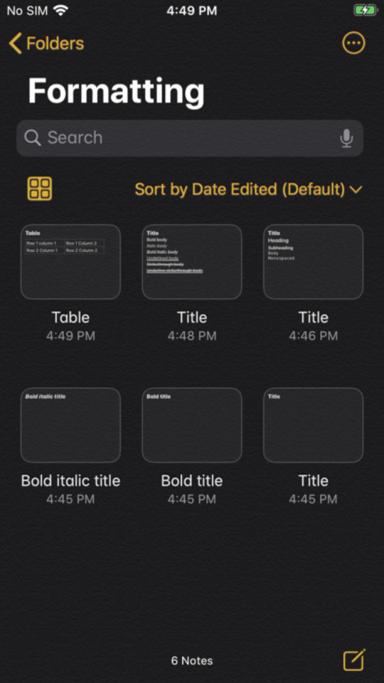
Although Apple does not directly document their Notes formats, the Developer Documents do provide insight into what you might expect to find. For example, Core Text is how text is laid out, which sounds a lot like what we were trying to find out in field 5. Reading these documents helped me understand some of the general ideas to be watching for.

What is in the Notes Protobuf Config?

Now that you know how you can iteratively build up a definition, I want to walk through the notestore.proto file which Apple Cloud Notes Parser uses. This could be easily imported to other projects in other languages besides Ruby and I am taking sections of the file out of order to build up a common understanding.

Note Protobuf

syntax = "proto2"; // // Classes related to the overall Note protobufs // // Overarching object in a ZNOTEDATA.ZDATA blob message NoteStoreProto { required Document document = 2; } // A Document has a Note within it. message Document { required int32 version = 2; required Note note = 3; } // A Note has both text, and then a lot of formatting entries. // Other fields are present and not yet included in this proto. message Note { required string note_text = 2; repeated AttributeRun attribute_run = 5; }

It seemed like what I found in poking at the protobufs fit the proto2 syntax better than the proto3 syntax, so that’s what I’m using. The NoteStoreProto, Document, and Note messages represent what we were looking at in the examples above, the highest level messages in the protobuf. As you can see, we don’t do much with the NoteStoreProto or Document and I would not be surprised to learn these have different names and a more general use in Apple. For the Note itself, the only two fields this .proto definition concerns itself with are 2 (the note text) and 5 (the attribute runs for formatting and the like).

// Represents a "run" of characters that need to be styled/displayed/etc message AttributeRun { required int32 length = 1; optional ParagraphStyle paragraph_style = 2; optional Font font = 3; optional int32 font_weight = 5; optional int32 underlined = 6; optional int32 strikethrough = 7; optional int32 superscript = 8; //Sign indicates super/sub optional string link = 9; optional Color color = 10; optional AttachmentInfo attachment_info = 12; } //Represents a color message Color { required float red = 1; required float green = 2; required float blue = 3; required float alpha = 4; } // Represents an attachment (embedded object) message AttachmentInfo { optional string attachment_identifier = 1; optional string type_uti = 2; } // Represents a font message Font { optional string font_name = 1; optional float point_size = 2; optional int32 font_hints = 3; } // Styles a "Paragraph" (any run of characters in an AttributeRun) message ParagraphStyle { optional int32 style_type = 1 [default = -1]; optional int32 alignment = 2; optional int32 indent_amount = 4; optional Checklist checklist = 5; } // Represents a checklist item message Checklist { required bytes uuid = 1; required int32 done = 2; }

Speaking of the AttributeRun, these are the messages which are needed to put it back together. Each of the AttributeRun messages have a length (field 1). They optionally have a lot of other fields, such as a ParagraphStyle (field 2), a Font (field 3), the various formatting booleans we saw above, a Color (field 10), and AttachmentInfo (field 12). The Color is pretty straight forward, taking RGB values. The AttachmentInfo is simple enough, just keeping the ZIDENTIFIER value and the ZTYPEUTI value. The Font isn’t something I actually take advantage of yet, but there are placeholders for the values which appear.

The ParagraphStyle is one of the more import messages for displaying a note as it helps to style a run of characters with information such as the indentation. It also contains within it a CheckList message, which holds the UUID of the checklist and whether or not it has been completed.

With the protobuf definition so far, you should be able to correctly render the text, although you will need a cheat sheet for the formatting found in ParagraphStyle’s first field. I originally had this in the protobuf definition, but I do not believe it is a true enum, so I moved it to the AppleNote class’ code as constants.

class AppleNote # Constants to reflect the types of styling in an AppleNote STYLE_TYPE_DEFAULT = -1 STYLE_TYPE_TITLE = 0 STYLE_TYPE_HEADING = 1 STYLE_TYPE_SUBHEADING = 2 STYLE_TYPE_MONOSPACED = 4 STYLE_TYPE_DOTTED_LIST = 100 STYLE_TYPE_DASHED_LIST = 101 STYLE_TYPE_NUMBERED_LIST = 102 STYLE_TYPE_CHECKBOX = 103 # Constants that reflect the types of font weighting FONT_TYPE_DEFAULT = 0 FONT_TYPE_BOLD = 1 FONT_TYPE_ITALIC = 2 FONT_TYPE_BOLD_ITALIC = 3 ... end

MergeableData protobuf

// // Classes related to embedded objects // // Represents the top level object in a ZMERGEABLEDATA cell message MergableDataProto { required MergableDataObject mergable_data_object = 2; } // Similar to Document for Notes, this is what holds the mergeable object message MergableDataObject { required int32 version = 2; // Asserted to be version in https://github.com/dunhamsteve/notesutils required MergeableDataObjectData mergeable_data_object_data = 3; } // This is the mergeable data object itself and has a lot of entries that are the parts of it // along with arrays of key, type, and UUID items, depending on type. message MergeableDataObjectData { repeated MergeableDataObjectEntry mergeable_data_object_entry = 3; repeated string mergeable_data_object_key_item = 4; repeated string mergeable_data_object_type_item = 5; repeated bytes mergeable_data_object_uuid_item = 6; } // Each entry is part of the pbject. For example, one entry might be identifying which // UUIDs are rows, and another might hold the text of a cell. message MergeableDataObjectEntry { required RegisterLatest register_latest = 1; optional Dictionary dictionary = 6; optional Note note = 10; optional MergeableDataObjectMap custom_map = 13; optional OrderedSet ordered_set = 16; }

Similar to the Note protobuf definition above, the MergeableDataProto and MergeableDataObject messages are likely larger objects which Notes just doesn’t have enough data to show the full understanding. MergeableDataObjectData (I know, the naming could use some work, that’s a future improvement) is really the embedded object found in the ZMERGEABLEDATA column. It is made up of a lot of MergeableDataObjectEntry messages (field 1) and the example from embedded tables is that an entry might tell the user which other entries are rows or columns. The MergeableDataObjectData also has strings which represent the key (field 4) or the type of item (field 5), and a set of 16 bytes which represent a UUID to identify this object (field 6).

MergeableDataObjectEntry is where things get more complicated. So far five of its fields seem relevant, with the Note message in field 10 already having been explained above. The RegisterLatest (field 1), Dictionary (field 6), MergeableDataObjectMap (field 13), and OrderedSet (field 16) objects are explained below, but will make the msot sense if you read about embedded tables at the same time.

// ObjectIDs are used to identify objects within the protobuf, offsets in an array, or // a simple String. message ObjectID { required uint64 unsigned_integer_value = 2; required string string_value = 4; required int32 object_index = 6; } // Register Latest is used to identify the most recent version message RegisterLatest { required ObjectID contents = 2; }

The RegisterLatest object has one ObjectID within it (field 2). This message is used to identify which ObjectID is the latest version. This is needed because Notes can have more than one source, between your local device, shared iCloud accounts, and a web editor in iCloud. As updates are merged, you can have older edits present, which you don’t want to use.

The ObjectID itself is useful in more places. It is used heavily in embedded tables and has three different possible pointers, one for unsigned integers (field 2), one for strings (field 4), and one for objects (field 6). It should point to one of those three, as way seen below.

// The Object Map uses its type to identify what you are looking at and // then a map entry to do something with that value. message MergeableDataObjectMap { required int32 type = 1; repeated MapEntry map_entry = 3; } // MapEntries have a key that maps to an array of key items and a value that points to an object. message MapEntry { required int32 key = 1; required ObjectID value = 2; }

Now that the ObjectID message is defined, we can look at the MergeableDataObjectMap. This message has a type (field 1) and potentially a lot of MapEntry messages (field 3). The type will be meaningful when looked up from another place.

The MapEntry message has an integer key (field 1) and an ObjectID value (field 2). The ObjectID will point to something that is indicated by the key, either as an integer, string, or object.

// A Dictionary holds many DictionaryElements message Dictionary { repeated DictionaryElement element = 1; } // Represents an object that has pointers to a key and a value, asserting // somehow that the key object has to do with the value object. message DictionaryElement { required ObjectID key = 1; required ObjectID value = 2; }

The Directionary message has a lot of DictionaryElement messages (field 1) within it. Each DictionaryElement has a key (field 1) and a value (field 2), both of which are ObjectIDs. For example, the key might be an ObjectID which has an ObjectIndex of 20 and the value might be an ObjectID with an ObjectIndex of 19. That would say that whatever is contained in index 20 is how we understand what we do with whatever is in index 19.

// An ordered set is used to hold structural information for embedded tables message OrderedSet { required OrderedSetOrdering ordering = 1; required Dictionary elements = 2; } // The ordered set ordering identifies rows and columns in embedded tables, with an array // of the objects and contents that map lookup values to originals. message OrderedSetOrdering { required OrderedSetOrderingArray array = 1; required Dictionary contents = 2; } // This array holds both the text to replace and the array of UUIDs to tell what // embedded rows and columns are. message OrderedSetOrderingArray { required Note contents = 1; repeated OrderedSetOrderingArrayAttachment attachment = 2; } // This array identifies the UUIDs that are embedded table rows or columns message OrderedSetOrderingArrayAttachment { required int32 index = 1; required bytes uuid = 2; }

Finally, we have a set of messages related to OrderedSets. These are really key in tables (as are most of these more complicated messages we discuss) and kind of wrap around the messages we saw above (i.e. an ObjectID is likely pointing to an index in an OrderedSet). An OrderedSet message has an OrderedSetOrdering message (field 1) and a Dictionary (field 2). The OrderedSetOrdering message has an OrderedSetOrderingArray (field 1) and another Dictionary (field 2). The OrderedSetOrderingArray interestingly has a Note (field 1) and potentially many OrderedSetOrderingArrayAttachment messages (field 2). Finally, the OrderedSetOrderingArrayAttachment has an index (field 1) and a 16-byte UUID (field 2).

I would highly recommend checking out the blog post about embedded tables to get through these last three sections of the protobuf with an example to follow along.

Conclusion

Protobufs are an efficient way to store data, particularly when you have to interact with that same data or data schema from different languages. My understanding of the Apple Notes protobuf is certainly not complete, but at this point is generally good enough to support recreating the look of a note after parsing it. Most of the protobuf is straightforward, it is really when you get into embedded tables that things get crazy. At this point, you should have a good enough understanding to compile the Cloud Note Parser’s proto file for your target language and start playing with it yourself!

#IFTTT #Feedly

0 notes

t-baba · 5 years ago

Photo

D3 6.0, easy 3D text, Electron 10, and reimplementing promises

#503 — August 28, 2020

Unsubscribe | Read on the Web

JavaScript Weekly

ztext.js: A 3D Typography Effect for the Web — While it initially has a bit of a “WordArt” feel to it, this library actually adds a pretty neat effect to any text you can provide. This is also a good example of a project homepage, complete with demos and example code.

Bennett Feely

D3 6.0: The Data-Driven Document Library — The popular data visualization library (homepage) takes a step forward by switching out a few internal dependencies for better alternatives, adopts ES2015 (a.k.a. ES6) internally, and now passes events directly to listeners. Full list of changes. There’s also a 5.x to 6.0 migration guide for existing users.

Mike Bostock

Scout APM - A Developer’s Best Friend — Scout’s intuitive UI helps you quickly track down issues so you can get back to building your product. Rest easy knowing that Scout is tracking your app’s performance and hunting down small issues before they become large issues. Get started for free.

Scout APM sponsor

Danfo.js: A Pandas-like Library for JavaScript — An introduction to a new library (homepage) that provides high-performance, intuitive, and easy-to-use data structures for manipulating and processing structured data following a similar approach to Python’s Pandas library. GitHub repo.

Rising Odegua (Tensorflow)

Electron 10.0.0 Released — The popular cross-platform desktop app development framework reaches a big milestone, though despite hitting double digits, this isn’t really a feature packed released but more an evolution of an already winning formula. v10 steps up to Chromium 85, Node 12.1.3, and V8 8.5.

Electron Team

Debug Visualizer 2.0: Visualize Data Structures Live in VS Code — We first mentioned this a few months ago but it’s seen a lot of work and a v2.0 release since then. It provides rich visualizations of watched values and can be used to visualize ASTs, results tables, graphs, and more. VS Marketplace link.

Henning Dieterichs

💻 Jobs

Sr. Engineer @ Dutchie, Remote — Dutchie is the world's largest and fastest growing cannabis marketplace. Backed by Howard Schultz, Thrive, Gron & Casa Verde Capital.

DUTCHIE

Find a Job Through Vettery — Create a profile on Vettery to connect with hiring managers at startups and Fortune 500 companies. It's free for job-seekers.

Vettery

📚 Tutorials, Opinions and Stories

Minimal React: Getting Started with the Frontend Library — Dr. Axel explains how to get started with React while using as few libraries as possible, including his state management approach.

Dr. Axel Rauschmayer

A Leap of Faith: Committing to Open Source — Babel maintainer Henry Zhu talks about how he left his role at Adobe to become a full-time open source maintainer, touching upon his faith, the humanity of such a role, and the finances of making it a reality.

The ReadME Project (GitHub)

Faster CI/CD for All Your Software Projects - Try Buildkite ✅ — See how Shopify scaled from 300 to 1800 engineers while keeping their build times under 5 minutes.

Buildkite sponsor

The Headless: Guides to Learning Puppeteer and Playwright — Puppeteer and Playwright are both fantastic high level browser control APIs you can use from Node, whether for testing, automating actions on the Web, scraping, or more. Code examples are always useful when working with such tools and these guides help a lot in this regard.

Checkly

How To Build Your Own Comment System Using Firebase — Runs through how to add a comments section to your blog with Firebase, while learning the basics of Firebase along the way.

Aman Thakur

A Guide to Six Commonly Used React Component Libraries

Max Rozen

Don't Trust Default Timeouts — “Modern applications don’t crash; they hang. One of the main reasons for it is the assumption that the network is reliable. It isn’t.”

Roberto Vitillo

Guide: Get Started with OpenTelemetry in Node.js

Lightstep sponsor

Deno Built-in Tools: An Overview and Usage Guide

Craig Buckler

How I Contributed to Angular Components — A developer shares his experience as an Angular Component contributor.

Milko Venkov

🔧 Code & Tools

fastest-levenshtein: Performance Oriented Levenshtein Distance Implementation — Levenshtein distance is a metric for measuring the differences between two strings (usually). This claims to be the fastest JS implementation, but we’ll let benchmarks be the judge of that :-)

ka-weihe

Yarn 2.2 (The Package Manager and npm Alternative) Released — As well as being smaller and faster, a dedupe command has been added to deduplicate dependencies with overlapping ranges.

Maël Nison

Light Date ⏰: Fast and Lightweight Date Formatting for Node and Browser — Comes in at 157 bytes, is well-tested, compliant with Unicode standards on dates, and written in TypeScript.

Antoni Kepinski

Barebackups: Super-Simple Database Backups — We automatically backup your databases on a schedule. You can use our storage or bring your own S3 account for unlimited backup storage.

Barebackups sponsor

Carbonium: A 1KB Library for Easy DOM Manipulation — Edwin submitted this himself, so I’ll let him explain it in his own words: “It’s for people who don’t want to use a JavaScript framework, but want more than native DOM. It might remind you of jQuery, but this library is only around one kilobyte and only supports native DOM functionality.”

Edwin Martin

DNJS: A JavaScript Subset for Configuration Languages — You might think that JSON can already work as a configuration language but this goes a step further by allowing various other JavaScript features in order to be more dynamic. CUE and Dhall are other compelling options in this space.

Oliver Russell

FullCalendar: A Full Sized JavaScript Calendar Control — An interesting option if you want a Google Calendar style control for your own apps. Has connectors for React, Vue and Angular. The base version is MIT licensed, but there’s a ‘premium’ version too. v5.3.0 just came out.

Adam Shaw

file-type: Detect The File Type of a Buffer, Uint8Array, or ArrayBuffer — For example, give it the raw data from a PNG file, and it’ll tell you it’s a PNG file. Usable from both Node and browser.

Sindre Sorhus

React-PDF: Display PDFs in a React App As Easily As If They Were Images

Wojciech Maj

Meteor 1.11 Released

Filipe Névola

🕰 ICYMI (Some older stuff that's worth checking out...)

Need to get a better understanding of arrow functions? This article from Tania Rascia will help.

Sure, strictly speaking a string in JavaScript is a sequence of UTF-16 code units... but there's more to it.

Zara Cooper explains how to take advantage of schematics in Angular Material and ng2-charts to substantially reduce the time and work that goes into building a dashboard

In this intro to memoizaition Hicham Benjelloun shares how you can optimize a function (by avoiding computing the same things several times).

by via JavaScript Weekly https://ift.tt/3jmo1hQ

#Javascript Branding #Javascript Weekly

0 notes

wemakenoclaims · 5 years ago

Text

Data Management and Visualization - Week 2 - Running My First Program

Given the option to learn SAS or Python, I chose Python.

The purpose of this week’s program (besides just learning how to do anything in Python) was to look at the distribution of values for three variables in my data set. Distribution just means what the range of values are and how often individual values appear, which can be expressed as a raw count or a percentage.

As a reminder, I’m using the GapMinder dataset for my research, and my question involves armedforcesrate and co2emissions variables. Since the assignment required a third, I also chose polityscore. I could have chosen any of course, but this one in particular helped to illustrate frequency in a way my chosen variables didn’t so well--more on that below.

OBSERVATIONS ON DISTRIBUTION

Both the armedforcesrate and co2emissions variables had values that were essentially unique--no two countries had the same value, other than blanks. This means the frequency of every non-null value is 1, and the percentage of every non-null value is identical. Of course that is correct and is a possible distribution; it just doesn’t do a lot to show you how frequency gets calculated! (Side note, it seems we’d want to do something like group these into ranges, or even just apply aggressive rounding, if we wanted to say something meaningful about the distribution).

This was why polityscore became an attractive third variable. It had a limited range of possible values so there wasn’t going to be a 1-to-1 distribution, and turned out to have clear frequency differences such that it wasn’t an even x-to-x distribution either.

armedforcesrate

-The values show a relatively narrow range, 0% to 10.6385211%, plus 49 blanks/non-responses

-No value dominates distribution; in fact, other than blanks no two rows had the same value!

co2emissions

- The values show a very broad range from 132,000 to 334,220,872,333.333 metric tons, plus 13 blanks/non-responses

-No value dominates distribution; in fact, other than blanks no two rows had the same value!

polityscore

-Prescribed range from -10 to +10 (in integers only), plus 52 blanks/non-responses

-All the possible values occur, but with unequal frequency. For example, here are the top 6 values (the first being blanks)...

...shown as count...

52 10 33 8 19 9 15 7 13 -7 12

..and shown as percentage (i.e. multiple by 100 to convert to % format)

0.244131 10 0.154930 8 0.089202 9 0.070423 7 0.061033 -7 0.056338

Now onto the program and the results from which my observations above were derived.

MY PROGRAM

Note on a program issue: As of publishing time, my data does have the potential problem that it is being misinterpreted as strings, due to the blanks, rather than numerical. The lesson’s solution for this is the “convert_objects” syntax which has since been deprecated from Pandas, and the current solution for this is, at least based on my research, the “pandas.to_numeric function” which is currently giving me errors. Thus you will see those lines, such as data["polityscore"]=pandas.to_numeric(data["polityscore"]) , commented out in my program. I do not believe it has corrupted the results; on the other hand, I’m a newbie here, plus there could be impacts to subsequent programs/projects.

In my defense I have reached out to the forums for help, see https://www.coursera.org/learn/data-visualization/peer/DwLkL/running-your-first-program/discussions/threads/K4KMcNphEeqTNgq0HQJyhQ

UPDATE (8/9/2020 1719ET) I found two solutions to this problem. I did not incorporate them into the program below since I figured I shouldn’t edit the substance of the post after submitting--for all I know someone has already reviewed and graded mine--but I did want to post the corrections.

data["polityscore"]=pandas.to_numeric(data["polityscore"]) is the same as data["polityscore"]=pandas.to_numeric(data["polityscore"],errors=“raise”) by implication, and raises an error message when data is found that doesn’t conform. In this case, the blanks were errors and the error messages I was seeing were per design; i.e. I hadn’t told pandas to do anything about them.

data["polityscore"]=pandas.to_numeric(data["polityscore"],errors=“coerce”) does what I’m looking for, replacing the blanks with NaN. Once I changed this my results showed nan rather than a blank space for those cases. Again, you won’t see that below because I didn’t make the corrections in the post itself since this was already submitted.

Also, looks like another variation of this which works is data["polityscore"] = data["polityscore"].apply(pandas.to_numeric,errors="coerce"). I am not versed enough in Python to explain the difference between it and the version I used.

# -*- coding: utf-8 -*- # import pandas module import pandas

#import numpy module (as of 8/9/2020, unused in my programs) import numpy

#statement to avoid run time error# pandas.set_option('display.float_format',lambda x:'%f'%x)

#statement to set max rows for the long lists associated with distro of two of my variables pandas.options.display.max_rows = 300

#read in the data from the GapMinder dataset, and convert the column names to lowercase data = pandas.read_csv ('_7548339a20b4e1d06571333baf47b8df_gapminder.csv', low_memory = False) data.columns = map (str.lower, data.columns)

#ensure numerical values are not misinterpreted as strings due to blanks ##disabled as of 8/9/2020 as neither the lesson syntax 'covert_objects' nor the syntax for the new command 'to_numeric' are working for me. ##posted question on forum, https://www.coursera.org/learn/data-visualization/peer/DwLkL/running-your-first-program/discussions/threads/K4KMcNphEeqTNgq0HQJyhQ ###data["polityscore"]=pandas.to_numeric(data["polityscore"]) ###data['co2emissions']=pandas.to_numeric(data['co2emissions']) ###data['armedforcesrate']=pandas.to_numeric(data['armedforcesrate'])

#display the number of rows and number of columns in the dataset print("Number of rows/observations--in this case, countries--in the dataset") print(len(data)) print("Number of columns/variables in the data set") print(len(data.columns)) print("")

#display the distribution counts for a chosen variable, with a descriptive name print("Distribution, by count, of the percent of total labor force in the armed forces") af1=data["armedforcesrate"].value_counts (dropna=False) print(af1) print("")

#display the distribution percentages for a chosen variable, with a descriptive name print("Distribution, by percentage, of the percent of total labor force in the armed forces") af2=data["armedforcesrate"].value_counts (normalize = True, dropna=False) print(af2) print("")

#display the distribution counts for a chosen variable, with a descriptive name print("Distribution, by count, of cumulative CO2 Emissions in metric tons") co1=data["co2emissions"].value_counts (dropna=False) print(co1) print("")

#display the distribution percentages for a chosen variable, with a descriptive name print("Distribution, by percentage, of cumulative CO2 Emissions in metric tons") co2=data["co2emissions"].value_counts (normalize = True, dropna=False) print(co2) print("")

#explanation slash apology print("NOTE on Armed Forces Rate and CO2 Emissions distributions") print("Other than blanks, no two countries in the dataset had the same values so the distribution is 1 (or the equivalent percentage share) for every value.") print("")

#display the distribution counts for a chosen variable, with a descriptive name print("Distribution, by count, of national polity scores, from -10 to 10, with -10 being fully autocratic and 10 being fully democratic") p1=data["polityscore"].value_counts (dropna=False) print(p1) print("")

#display the distribution percentages for a chosen variable, with a descriptive name print("Distribution, by percentage, of national polity scores, from -10 to 10, with -10 being fully autocratic and 10 being fully democratic") p2=data["polityscore"].value_counts (normalize = True, dropna=False) print(p2) print("//End of output//")

MY OUTPUT

Note on a reader attention issue: If your eyes are glazing over reading the 200+ entries for armedforcesdatarate and co2emissions, where every non-blank value was unique, you might want to skip down to polityscore!

Python 3.8.3 (default, Jul 2 2020, 17:30:36) [MSC v.1916 64 bit (AMD64)]

Type "copyright", "credits" or "license" for more information.

IPython 7.16.1 -- An enhanced Interactive Python.

runfile('C:/Users/Matt/Documents/Python Scripts/GapMinder_p2.py', wdir='C:/Users/Matt/Documents/Python Scripts') Number of rows/observations--in this case, countries--in the dataset 213 Number of columns/variables in the data set 16

Distribution, by count, of the percent of total labor force in the armed forces 49 .5235483 1 .8668624 1 .5415062 1 5.9360854 1 2.3162346 1 5.8731426 1 1.9129653 1 .5159403 1 7.7379125 1 .3976544 1 1.3342359 1 .9984276 1 2.4549129 1 .969499 1 .7502103 1 .7583556 1 2.0433877 1 .3891575 1 2.5364458 1 .5739204 1 .1299529 1 .4026995 1 1.7293464 1 .8101865 1 1.1421267 1 1.012373 1 .5758096 1 1.1319097 1 1.4507353 1 1.0247361 1 .9723782 1 1.3411144 1 1.1774157 1 .7108232 1 .8776657 1 1.1032787 1 .3713568 1 .4833248 1 2.8339665 1 1.5793413 1 .2351846 1 .6123401 1 0 1 2.306817 1 3.3116742 1 .0661 1 .2339148 1 1.9767462 1 .8358123 1 1.266624 1 .2176526 1 6.3949358 1 2.0858528 1 .5452863 1 2.2156207 1 .5157058 1 .7213964 1 2.569643 1 .3445177 1 .1345905 1 .1314868 1 .3622613 1 .2177167 1 .5080181 1 .7096295 1 2.3794147 1 .5265916 1 1.6494507 1 1.1602817 1 1.5512617 1 4.3015761 1 1.4613288 1 .1145925 1 .3880673 1 3.4515458 1 .1022692 1 1.616886 1 1.0189063 1 1.0584191 1 .3618584 1 3.2908071 1 .3269778 1 .9562696 1 .305758 1 .7268554 1 10.6385211 1 4.4659976 1 .52422 1 .4862799 1 .9040245 1 5.9558471 1 2.6182964 1 1.8124763 1 3.0932506 1 .2233986 1 .9311688 1 .1051147 1 .1486587 1 1.1772684 1 .1595738 1 .2437395 1 2.101467 1 .628381 1 1.8821978 1 .8155798 1 5.4065355 1 .4500244 1 1.9414459 1 .7313362 1 .1347296 1 1.2118685 1 .5696534 1 1.6095482 1 1.4878309 1 1.4356332 1 .8156477 1 .3429763 1 1.0853671 1 2.6184384 1 .6639555 1 .7716936 1 1.2337802 1 .6048733 1 .9314175 1 1.0179463 1 .3617085 1 1.1443188 1 1.0936515 1 1.5367663 1 9.8201265 1 .2342862 1 5.9096991 1 .3331953 1 .1629041 1 .5261262 1 1.1577498 1 1.9729132 1 .581165 1 .9301079 1 .9795374 1 1.0127322 1 .3495439 1 5.2311429 1 2.0263996 1 .4736536 1 4.683989 1 3.7119299 1 1.3164321 1 .2878915 1 1.321155 1 .628578 1 .4628471 1 .6608385 1 1.4953835 1 .3400308 1 1.0327854 1 .3520917 1 .885386 1 .3318626 1 .8377678 1 1.469369 1 .560987 1 .3413352 1 .7205279 1 Name: armedforcesrate, dtype: int64

Distribution, by percentage, of the percent of total labor force in the armed forces 0.230047 .5235483 0.004695 .8668624 0.004695 .5415062 0.004695 5.9360854 0.004695 2.3162346 0.004695 5.8731426 0.004695 1.9129653 0.004695 .5159403 0.004695 7.7379125 0.004695 .3976544 0.004695 1.3342359 0.004695 .9984276 0.004695 2.4549129 0.004695 .969499 0.004695 .7502103 0.004695 .7583556 0.004695 2.0433877 0.004695 .3891575 0.004695 2.5364458 0.004695 .5739204 0.004695 .1299529 0.004695 .4026995 0.004695 1.7293464 0.004695 .8101865 0.004695 1.1421267 0.004695 1.012373 0.004695 .5758096 0.004695 1.1319097 0.004695 1.4507353 0.004695 1.0247361 0.004695 .9723782 0.004695 1.3411144 0.004695 1.1774157 0.004695 .7108232 0.004695 .8776657 0.004695 1.1032787 0.004695 .3713568 0.004695 .4833248 0.004695 2.8339665 0.004695 1.5793413 0.004695 .2351846 0.004695 .6123401 0.004695 0 0.004695 2.306817 0.004695 3.3116742 0.004695 .0661 0.004695 .2339148 0.004695 1.9767462 0.004695 .8358123 0.004695 1.266624 0.004695 .2176526 0.004695 6.3949358 0.004695 2.0858528 0.004695 .5452863 0.004695 2.2156207 0.004695 .5157058 0.004695 .7213964 0.004695 2.569643 0.004695 .3445177 0.004695 .1345905 0.004695 .1314868 0.004695 .3622613 0.004695 .2177167 0.004695 .5080181 0.004695 .7096295 0.004695 2.3794147 0.004695 .5265916 0.004695 1.6494507 0.004695 1.1602817 0.004695 1.5512617 0.004695 4.3015761 0.004695 1.4613288 0.004695 .1145925 0.004695 .3880673 0.004695 3.4515458 0.004695 .1022692 0.004695 1.616886 0.004695 1.0189063 0.004695 1.0584191 0.004695 .3618584 0.004695 3.2908071 0.004695 .3269778 0.004695 .9562696 0.004695 .305758 0.004695 .7268554 0.004695 10.6385211 0.004695 4.4659976 0.004695 .52422 0.004695 .4862799 0.004695 .9040245 0.004695 5.9558471 0.004695 2.6182964 0.004695 1.8124763 0.004695 3.0932506 0.004695 .2233986 0.004695 .9311688 0.004695 .1051147 0.004695 .1486587 0.004695 1.1772684 0.004695 .1595738 0.004695 .2437395 0.004695 2.101467 0.004695 .628381 0.004695 1.8821978 0.004695 .8155798 0.004695 5.4065355 0.004695 .4500244 0.004695 1.9414459 0.004695 .7313362 0.004695 .1347296 0.004695 1.2118685 0.004695 .5696534 0.004695 1.6095482 0.004695 1.4878309 0.004695 1.4356332 0.004695 .8156477 0.004695 .3429763 0.004695 1.0853671 0.004695 2.6184384 0.004695 .6639555 0.004695 .7716936 0.004695 1.2337802 0.004695 .6048733 0.004695 .9314175 0.004695 1.0179463 0.004695 .3617085 0.004695 1.1443188 0.004695 1.0936515 0.004695 1.5367663 0.004695 9.8201265 0.004695 .2342862 0.004695 5.9096991 0.004695 .3331953 0.004695 .1629041 0.004695 .5261262 0.004695 1.1577498 0.004695 1.9729132 0.004695 .581165 0.004695 .9301079 0.004695 .9795374 0.004695 1.0127322 0.004695 .3495439 0.004695 5.2311429 0.004695 2.0263996 0.004695 .4736536 0.004695 4.683989 0.004695 3.7119299 0.004695 1.3164321 0.004695 .2878915 0.004695 1.321155 0.004695 .628578 0.004695 .4628471 0.004695 .6608385 0.004695 1.4953835 0.004695 .3400308 0.004695 1.0327854 0.004695 .3520917 0.004695 .885386 0.004695 .3318626 0.004695 .8377678 0.004695 1.469369 0.004695 .560987 0.004695 .3413352 0.004695 .7205279 0.004695 Name: armedforcesrate, dtype: float64

Distribution, by count, of cumulative CO2 Emissions in metric tons 13 1111000 1 7601000 1 4200940333.33333 1 100782000 1 188268666.666667 1 170404666.666667 1 283583666.666667 1 236419333.333333 1 225019666.666667 1 1436893333.33333 1 56818666.6666667 1 1414031666.66667 1 20331666.6666667 1 531303666.666667 1 2712915333.33333 1 334220872333.333 1 23635333.3333333 1 46092214666.6667 1 1045000 1 19800000 1 377303666.666667 1 2315698000 1 254206333.333333 1 2269806000 1 1206333.33333333 1 300934333.333333 1 2406741333.33333 1 20152000 1 692039333.333333 1 590674333.333333 1 125172666.666667 1 4774000 1 26125000 1 4286590000 1 1839471333.33333 1 428006333.333333 1 16379000 1 7608333.33333334 1 592012666.666667 1 23053598333.3333 1 40857666.6666667 1 52657000 1 41229554666.6667 1 143586666.666667 1 127108666.666667 1 14241333.3333333 1 24979045666.6667 1 183535000 1 35717000 1 14609848000 1 1962704333.33333 1 22704000 1 2907666.66666667 1 104170000 1 23404568000 1 1286670000 1 132000 1 88337333.3333333 1 46684000 1 3157700333.33333 1 10822529666.6667 1 340090666.666667 1 1776016000 1 125755666.666667 1 73784333.3333333 1 170804333.333333 1 9183548000 1 107096000 1 2484925666.66667 1 9580226333.33333 1 2386820333.33333 1 2670950333.33333 1 21351000 1 109681000 1 38991333.3333333 1 242594000 1 5214000 1 1026813333.33333 1 5896388666.66667 1 7355333.33333333 1 7388333.33333334 1 310024000 1 2335666.66666667 1 2932108666.66667 1 62777000 1 49793333.3333333 1 275744333.333333 1 32233666.6666667 1 95256333.3333333 1 248358000 1 14054333.3333333 1 1561079666.66667 1 4244009000 1 36160666.6666667 1 234864666.666667 1 511107666.666667 1 850666.666666667 1 953051000 1 9155666.66666667 1 14058000 1 8092333.33333333 1 35871000 1 5584766000 1 3503877666.66667 1 148470666.666667 1 6024333.33333333 1 1425435000 1 5418886000 1 137555000 1 169180000 1 2251333.33333333 1 503994333.333333 1 26209333.3333333 1 1718339333.33333 1 17515666.6666667 1 72524250333.3333 1 7315000 1 10897025333.3333 1 29758666.6666667 1 59473333.3333333 1 56162333.3333333 1 8231666.66666667 1 2420300666.66667 1 228748666.666667 1 131703000 1 2977333.33333333 1 4352333.33333334 1 253854333.333333 1 51219666.6666667 1 598774000 1 999874333.333333 1 214368000 1 1548044666.66667 1 16225000 1 9483023000 1 12970092666.6667 1 132025666.666667 1 5675629666.66667 1 86317000 1 226255333.333333 1 2368666.66666667 1 8968666.66666667 1 811965000 1 20628666.6666667 1 1633778666.66667 1 590219666.666666 1 8338000 1 1723333.33333333 1 30800000 1 55146666.6666667 1 5248815000 1 446365333.333333 1 38397333.3333333 1 5210333.33333334 1 3659333.33333333 1 1865922666.66667 1 102538333.333333 1 87970666.6666667 1 223747333.333333 1 119958666.666667 1 69329333.3333333 1 7104137333.33333 1 46306333.3333333 1 149904333.333333 1 101386215333.333 1 75944000 1 81191000 1 4814333.33333333 1 5872119000 1 4466084333.33333 1 92770333.3333334 1 45411666.6666667 1 1712755000 1 78943333.3333333 1 322960000 1 37950000 1 2329308666.66667 1 254939666.666667 1 7861553333.33333 1 525891666.666667 1 2401666.66666667 1 1146277000 1 90269666.6666667 1 2421917666.66667 1 13304503666.6667 1 6710201666.66667 1 45778333.3333333 1 277170666.666667 1 30391317000 1 1321661000 1 9666891666.66666 1 3341129000 1 7813666.66666667 1 33341634333.3333 1 168883000 1 21332666.6666667 1 487993000 1 28490000 1 19000454000 1 2008116000 1 Name: co2emissions, dtype: int64

Distribution, by percentage, of cumulative CO2 Emissions in metric tons 0.061033 1111000 0.004695 7601000 0.004695 4200940333.33333 0.004695 100782000 0.004695 188268666.666667 0.004695 170404666.666667 0.004695 283583666.666667 0.004695 236419333.333333 0.004695 225019666.666667 0.004695 1436893333.33333 0.004695 56818666.6666667 0.004695 1414031666.66667 0.004695 20331666.6666667 0.004695 531303666.666667 0.004695 2712915333.33333 0.004695 334220872333.333 0.004695 23635333.3333333 0.004695 46092214666.6667 0.004695 1045000 0.004695 19800000 0.004695 377303666.666667 0.004695 2315698000 0.004695 254206333.333333 0.004695 2269806000 0.004695 1206333.33333333 0.004695 300934333.333333 0.004695 2406741333.33333 0.004695 20152000 0.004695 692039333.333333 0.004695 590674333.333333 0.004695 125172666.666667 0.004695 4774000 0.004695 26125000 0.004695 4286590000 0.004695 1839471333.33333 0.004695 428006333.333333 0.004695 16379000 0.004695 7608333.33333334 0.004695 592012666.666667 0.004695 23053598333.3333 0.004695 40857666.6666667 0.004695 52657000 0.004695 41229554666.6667 0.004695 143586666.666667 0.004695 127108666.666667 0.004695 14241333.3333333 0.004695 24979045666.6667 0.004695 183535000 0.004695 35717000 0.004695 14609848000 0.004695 1962704333.33333 0.004695 22704000 0.004695 2907666.66666667 0.004695 104170000 0.004695 23404568000 0.004695 1286670000 0.004695 132000 0.004695 88337333.3333333 0.004695 46684000 0.004695 3157700333.33333 0.004695 10822529666.6667 0.004695 340090666.666667 0.004695 1776016000 0.004695 125755666.666667 0.004695 73784333.3333333 0.004695 170804333.333333 0.004695 9183548000 0.004695 107096000 0.004695 2484925666.66667 0.004695 9580226333.33333 0.004695 2386820333.33333 0.004695 2670950333.33333 0.004695 21351000 0.004695 109681000 0.004695 38991333.3333333 0.004695 242594000 0.004695 5214000 0.004695 1026813333.33333 0.004695 5896388666.66667 0.004695 7355333.33333333 0.004695 7388333.33333334 0.004695 310024000 0.004695 2335666.66666667 0.004695 2932108666.66667 0.004695 62777000 0.004695 49793333.3333333 0.004695 275744333.333333 0.004695 32233666.6666667 0.004695 95256333.3333333 0.004695 248358000 0.004695 14054333.3333333 0.004695 1561079666.66667 0.004695 4244009000 0.004695 36160666.6666667 0.004695 234864666.666667 0.004695 511107666.666667 0.004695 850666.666666667 0.004695 953051000 0.004695 9155666.66666667 0.004695 14058000 0.004695 8092333.33333333 0.004695 35871000 0.004695 5584766000 0.004695 3503877666.66667 0.004695 148470666.666667 0.004695 6024333.33333333 0.004695 1425435000 0.004695 5418886000 0.004695 137555000 0.004695 169180000 0.004695 2251333.33333333 0.004695 503994333.333333 0.004695 26209333.3333333 0.004695 1718339333.33333 0.004695 17515666.6666667 0.004695 72524250333.3333 0.004695 7315000 0.004695 10897025333.3333 0.004695 29758666.6666667 0.004695 59473333.3333333 0.004695 56162333.3333333 0.004695 8231666.66666667 0.004695 2420300666.66667 0.004695 228748666.666667 0.004695 131703000 0.004695 2977333.33333333 0.004695 4352333.33333334 0.004695 253854333.333333 0.004695 51219666.6666667 0.004695 598774000 0.004695 999874333.333333 0.004695 214368000 0.004695 1548044666.66667 0.004695 16225000 0.004695 9483023000 0.004695 12970092666.6667 0.004695 132025666.666667 0.004695 5675629666.66667 0.004695 86317000 0.004695 226255333.333333 0.004695 2368666.66666667 0.004695 8968666.66666667 0.004695 811965000 0.004695 20628666.6666667 0.004695 1633778666.66667 0.004695 590219666.666666 0.004695 8338000 0.004695 1723333.33333333 0.004695 30800000 0.004695 55146666.6666667 0.004695 5248815000 0.004695 446365333.333333 0.004695 38397333.3333333 0.004695 5210333.33333334 0.004695 3659333.33333333 0.004695 1865922666.66667 0.004695 102538333.333333 0.004695 87970666.6666667 0.004695 223747333.333333 0.004695 119958666.666667 0.004695 69329333.3333333 0.004695 7104137333.33333 0.004695 46306333.3333333 0.004695 149904333.333333 0.004695 101386215333.333 0.004695 75944000 0.004695 81191000 0.004695 4814333.33333333 0.004695 5872119000 0.004695 4466084333.33333 0.004695 92770333.3333334 0.004695 45411666.6666667 0.004695 1712755000 0.004695 78943333.3333333 0.004695 322960000 0.004695 37950000 0.004695 2329308666.66667 0.004695 254939666.666667 0.004695 7861553333.33333 0.004695 525891666.666667 0.004695 2401666.66666667 0.004695 1146277000 0.004695 90269666.6666667 0.004695 2421917666.66667 0.004695 13304503666.6667 0.004695 6710201666.66667 0.004695 45778333.3333333 0.004695 277170666.666667 0.004695 30391317000 0.004695 1321661000 0.004695 9666891666.66666 0.004695 3341129000 0.004695 7813666.66666667 0.004695 33341634333.3333 0.004695 168883000 0.004695 21332666.6666667 0.004695 487993000 0.004695 28490000 0.004695 19000454000 0.004695 2008116000 0.004695 Name: co2emissions, dtype: float64

NOTE on Armed Forces Rate and CO2 Emissions distributions Other than blanks, no two countries in the dataset had the same values so the distribution is 1 (or the equivalent percentage share) for every value.

Distribution, by count, of national polity scores, from -10 to 10, with -10 being fully autocratic and 10 being fully democratic 52 10 33 8 19 9 15 7 13 -7 12 6 10 5 7 -3 6 0 6 -4 6 -2 5 4 4 -9 4 -1 4 1 3 2 3 -6 3 3 2 -5 2 -8 2 -10 2 Name: polityscore, dtype: int64

Distribution, by percentage, of national polity scores, from -10 to 10, with -10 being fully autocratic and 10 being fully democratic 0.244131 10 0.154930 8 0.089202 9 0.070423 7 0.061033 -7 0.056338 6 0.046948 5 0.032864 -3 0.028169 0 0.028169 -4 0.028169 -2 0.023474 4 0.018779 -9 0.018779 -1 0.018779 1 0.014085 2 0.014085 -6 0.014085 3 0.009390 -5 0.009390 -8 0.009390 -10 0.009390 Name: polityscore, dtype: float64 //End of output//

0 notes