#DatabaseTables | Explore Tumblr posts and blogs

tototavros · 3 years ago

Note

What is Haskell used for? I can point to many languages and say, "oh, this is often used for thus and such" but I don't know what Haskell's common use cases are.

The main use of Haskell is in improving Haskell :P

Seriously, parser combinators are a great idea and easily expressed in Haskell, and so it's easy enough to write some basic parsers for a non-syntax heavy language, and a lot of the features are developed with this in mind (and has trickle down effects on serialization/deserialization libraries--Aeson is pretty good for dealing with JSON (de)serialization)

I really like it for writing backends with Servant (kind of like Flask in that it's not a batteries-included type of server library), although the errors are kind of confusing, especially if you're not used to Haskell already

There's a relatively Haskell-specific development of a thing called "monad transformers", which is an ugly term for a way to write capability-specific abstractions

For instance, if you have MonadDatabase or a DatabaseT in your type signature, then that function can call whatever functions are defined for MonadDatabase, be it get/set for some restricted types, or computing raw SQL...either way, it's obvious that if you're trying to use this to get the system time, you're using the wrong abstraction (and you can have multiple of these in your type signature, so you might have (Monad m) => AWSBucketT (TimeT (m Int)), which assuming some definitions, might say "In some monad m, I'll return an Int, and have capabilities to access our company's AWSBuckets and read the system time"

(Monad transformers as they're used often aren't great imo, but i've already gone too deep, perhaps too deep by even saying "monad")

Beyond that, a couple other useful things: you might know map from Python or Rust, but what if it was easier to automatically get a sensible definition of map? After all, there's usually only one "right answer"--apply the function to all relevant targets!

So say you have some type like data Tree e a = Leaf e | Node a [Tree e a]

(so, a Tree over e and a is either a `Leaf` that only has an `e`, or a Node, which is annotated with an `a`, and has a list of child trees over the same types)

then if you just add `derive Functor` to the end of the datatype, it'll create a map function that looks like:

map f (Leaf e) = Leaf e

map f (Node a trees) = Node (f a) [map f tree | tree <- trees]

(or in pythonish: def map(f, t): if t.isLeaf(): pass; else: t.value = f(t.value); t.children = [map(f, tree) for tree in t.children])

Say you want your map to effect the Leafs rather than the annotations of the Nodes, then all you need to do is flip the type variables, then you can just write it as data Tree a e = Leaf e | Node a [Tree a e] deriving Functor

There's similar derivings for Show (the default printing type) or JSON de/serialization among others. If you're familiar with Rust's derive macro, it's a similar thing

This isn't something one should choose a language *for* but i think it's pretty neat

Property testing is easy in Haskell, you assert some property that you think your funciton should have (say, f(f(x)) = f(x)), write a way to compare the output for equality (or derive it), write a way to generate your inputs (or derive it, you can also easily customise it thanks to the combinators), and then your computer will generate however many "unit tests" that you want, and then check them all at once against the property. (There's an extension to this where if you put an ordering of "complexity", the property testing library will often try to find the "simplest" (according to your definition) input that violates the property.)

The pattern matching/equational definition of functions is something that I like a lot, there's a case analyzer built into the compiler that tells you when you've neglected a case (or added a case to a datatype), and there's extensions for IDEs that will show this as a linting message

Some other things that Haskell's used for is HPC (supposedly the FFI isn't awful, and implementing a really basic version of Map/Reduce in Haskell is pretty trivial, thanks to the thought put into async + threaded programming (it has problems and footguns, just mostly different ones than you're used to except for "the fuck is the runtime doing"; that just happens, and the GHC RTS i hear is like an abyss of phd theses)

There's also a healthy niche of circuit design(?), thanks to the deep support for embedded dsls; I'd recommend going through https://hackage.haskell.org/package/clash-ghc or Conal Elliot's work

Finally, Haskell is a language that tries to be on the forefront of language design. This means that a lot of useless and confusing features have snuck into the language, although usually they're gatekept behind compiler extensions. However, a lot of neat things show up early on in the Haskell world, before a lot of other programming languages pick up the features! I've already mentioned the deriving feature similar to Rust, it also has a linear types extension (tho support is limited as its a recent addition), and was a breeding ground for reactive programming iirc (React makes a lot more sense than Haskell's similar libraries tho)

#long post #trying not to be too technical while also being correct #i'm bad at selling haskell because it just feels so much comfier to me than any other language for a bunch of reasons that seem minor #but stack up #capability based programming good #equational function defintions good #the freedom of expression while also being constrained to reasonableness is good #definitely rambling

12 notes · View notes

tak4hir0 · 5 years ago

Link

At the core of Tableau is data - your data. Your data can come in different formats and structures, categorized at varying levels of detail, and can have relationships with other data. This is the kind of metadata that you can expect to surface from the Metadata API using GraphQL. In order to successfully create effective GraphQL queries, you need to understand how Tableau interprets and interacts with content and assets. Understanding this can inform the most efficient way for you to access metadata at the level of detail that you need. Because the Metadata API uses GraphQL, this section describes the fundamental objects that are available to you to use in a GraphQL query. In this section Tableau content and assets Objects and their roles Object types and inherited attributes Other objects related to Tableau content and assets Tableau metadata model Example metadata model Example scenario 1: Impact analysis Example scenario 2: Lineage analysis Additional notes about the metadata model Tableau content and assets The Metadata API surfaces the content and assets that comprise your Tableau Online site or Tableau Server, the content and asset roles, and how the content and assets relate to each other. General Tableau content Tableau content is unique to the Tableau platform. Content includes the following: Data sources - both published and embedded Workbooks Sheets - including dashboards and stories Fields: calculated, column - as they relate to the data source, group, bin, set, hierarchy, combined, and combined set Filters: data source Parameters Flows Tableau Online and Tableau Server specific content Tableau content that can only be managed through Tableau Online or Tableau Server includes the following: Sites Projects Users Certifications and certifiers Data quality warnings and messages Note: Some content listed above can be managed through the Tableau Server REST API as well. External assets associated with Tableau content The Metadata API treats information about any data that comes from outside of the Tableau environment as external assets. External assets include the following: Databases - includes local files, remote connections to servers, and web data connectors (WDC) Tables - includes queries (custom SQL) Objects and their roles The GraphQL schema used by the Metadata API organizes content and assets on Tableau Online and Tableau Server by grouping them by object and role. These objects and their roles are the foundation to your GraphQL queries. Parent object and role Parent objects, a mix of both content and assets, can be managed independently of other objects and play the role of a container. Parent objects can refer to other parent objects, can refer to child objects, and can also own child objects. Parent objects Databases Tables Published data sources Workbooks Flows Sites Projects Users Child object and role Child objects, also a mix of both content and assets, cannot be managed independently of their parent object. Therefore, child objects play a dependent role on their parent object. Some child objects can own other child objects, can refer to other child objects, and in some cases, refer to certain parent objects. Child objects Columns Fields Embedded data sources Sheets Aliases Parameters Data source filters Parent/child object relationship The GraphQL schema defines the parent/child object relationship by what the objects can own or contain. In other words, an object is a parent object when it functions as a container for other (child) objects. Parent object Can own or contain objects... DatabaseServer CloudFileCustomSqlTableDatabaseTableFileWebDataConnector DatabaseTable Column PublishedDataSource DataSourceFilterAnalyticsFieldBinFieldCalculatedFieldColumnFieldCombinedFieldCombinedSetFieldDataSourceFieldGroupFieldHierarchyFieldSetField Workbook EmbeddedDataSourceDashboardSheet Sheet Field??(sheet type - e.g., calculated fields created in the Row or Column shelf) Flow FlowInputFieldFlowOutputField TableauSite - TableauProject - User - Object types and inherited attributes Parallel to parent/child object role and relationship, the GraphQL schema organizes objects by object type and the attributes that it can inherit from the object. To do this, objects are implemented in the GraphQL schema using “interfaces.” From each interface, object types inherit attributes and properties. This means that the object types that have the same interface have a logical association with each other and share common attributes and properties. In addition to the shared attributes and properties, object types can also have unique attributes and properties. Examples of object types and their inherited attributes The table below captures example objects, object types (interface), and their common and unique attributes and properties. Object Object type or interface Common attributes and properties Unique attributes and properties Database CloudFileDatabaseServerFileWebDataConnector idvizportalidluidnamehostnameportisEmbeddedconnectionTypedescriptioncontactisControlledPermissionsEnabledisCertifiedcertificationNotecertifiertablestablesConnectiondatatQualityWarninghasActiveWarningservice CloudFile providerfileExtensionmimeTypefieldrequestUrl DatabaseServer extendedConnectionTypehostNameport File filePath WebDataConnector connectorUrl Table DatabaseTableCustomSQLTable idnameisEmbeddeddescriptionisCertifiedcertificationNote CustomSQLTable query DatabaseTable luidvizportalIdschemafullNamecontact Datasource PublishedDatasourceEmbeddedDatasource idnamehasUserReferencehasExtractsextractLastRefreshTimeextractLastUpdateTimeextractLastIncrementalUpdateTimeextractLastUpdateTimefieldsfieldsConnectiondatasourceFiltersdatasourceFiltersConnection PublishedDataSource luidparametersparametersConnectionsiteprojectownerisCertifiedcertifiercertificationNotecertifierDisplayNamedescriptionurivizportalURLId EmbeddedDatasource workbook Warnable (data quality warning) CloudFileDatabaseServerFileWebDataConnectorDatabaseTablePublishedDatasourceFlow idhasActiveWarningdataQualityWarning - Other objects related to Tableau content and assets Lineage shortcut objects The Metadata API enables you to see relationships between the content and asset that you’re evaluating with other items on your Tableau Online site or Tableau Server. These items include the following: Upstream and downstream content - including data sources, workbooks, sheets, fields, flows, and owners Upstream and downstream assets - including databases, tables, and columns You can quickly access this type of information by using shortcut objects defined in the GraphQL schema. These lineage or relationship objects use the upstream or downstream prefix. For example, you can use upstreamTablesConnection to query the tables used by a data source or use downstreamSheetsConnection to query sheets used by a workbook. For an example query that uses lineage shortcut, see Filtering section in the Example Queries topic. Pagination objects The Metadata API enables you to traverse through relationships within the data that you’re querying using pagination. The GraphQL schema defines pagination objects as those objects that use the Connection suffix. For example, you can use the databasesConnection to get a list of paginated results of database assets on your Tableau Online site or Tableau Server. For an example query that uses pagination, see Pagination section in the Example Queries topic. Together, all objects, the roles they play, the relationships they have with each other and their attributes and properties define the metadata model for a particular set of objects. The metadata model is a snapshot (or in GraphQL terms, a graph) of how Tableau interprets and relates a set of objects on your Tableau Online site or Tableau Server. From the metadata model, you can understand the dependencies and relationships in your data. To see how the metadata model used by the Metadata API works, review the following example scenarios. Example metadata model Suppose you have three workbooks (parent objects) and two data sources (parent objects) published to Tableau Online or Tableau Server. For this scenario, the two published data source objects refer to the three workbook objects. The workbook objects own four sheet objects. These sheet objects in turn refer to two field objects that are owned by the published data source objects. Here’s what the metadata model for this scenario might look like. Notes: A sold line with an arrow indicates a ownership relationship. A dotted line indicates a reference relationship. Example scenario 1: Impact analysis In an impact analysis scenario, the metadata model can help you answer how data might be affected if a part of the metadata model changes. In this scenario, you might want to know what could happen if the published data source, John County - 1, is deleted. As you know now from the metadata model, sheet objects are owned by workbook objects, and sheet objects can refer to the field objects. In this scenario, the field objects are owned by the published data source objects. Published data source objects own field objects. Therefore, if John County - 1 is deleted, the child objects, F1, Hills Library, and Garden Library, are directly affected and their existence compromised because of their dependency on that data source object. The other child objects, F2, Garden Senior Center, and Cliff Senior Center, though they might be affected by the data source object being deleted, their existence is not compromised. During this analysis, you can see that because John County - 1 doesn’t own the workbook objects that connect to it, the workbook objects themselves, both Sakura District and Maple District can continue to exist in the absence of the published data source object. Example scenario 2: Lineage analysis In a lineage flow analysis scenario, you can look at particular part of the metadata model and identify where the data is coming from and how the data reacts or is affected by different parts of the metadata model. In this scenario, you might want to know where a data point from a sheet object, Garden Senior Center, in a workbook object, Maple District, is coming from. Based on what you know from the metadata model, attributes are inherited from the parent object . Therefore, if you start from Garden Senior Center sheet object, you can move to the referring field object, F2, to see that it’s owned by a published data source object. In this case, John County - 2 is the source for the data point. During this analysis, you are able to freely include or exclude parts of the metadata model in order to understand the lineage flow for Garden Senior Center. For example, you can choose to exclude Garden Library sheet object even though it’s also owned by the same workbook object, Maple District. Additional notes about the metadata model When using custom SQL The metadata model interprets customSQL queries as tables. When custom SQL queries are defined in your data source or flow, the queries have to fit a set of criteria to be recognized and interpreted by the Metadata API. For more information, see Tableau Catalog support for custom SQL in the Tableau Help. When using the databaseTable object in a query When you run a query using the databaseTable object, for some databases, the schema attribute might not return the correct schema name for the table. This issue can occur when the selected schema, while creating or editing a data source, workbook, or flow, is changed after adding the table. When the selected schema changes after adding the table, the schema attribute your query returns is the name of the last selected schema instead of the actual schema that the table is using. Databases that might return the incorrect schema in the scenario described above include Amazon Athena and Exasol.

#help.tableau.com

0 notes

datadario · 8 years ago

Text

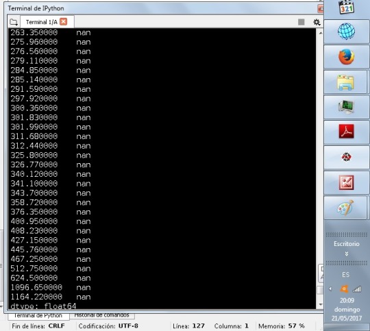
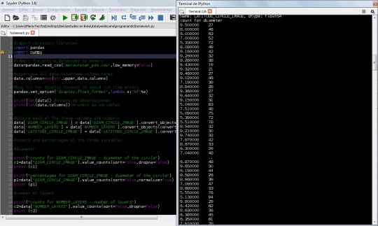
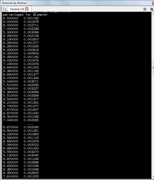
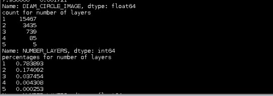
homework week 4

The program is the next

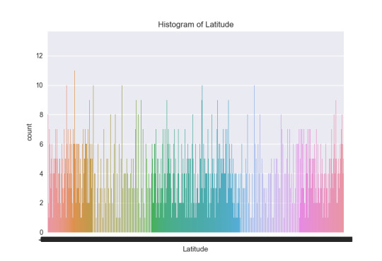
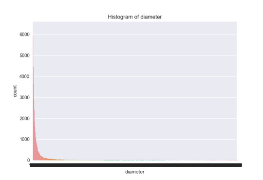
# -*- coding: utf-8 -*- """ Created on Sun May 21 15:06:26 2017 @author: Dario Suing """ #import necessary libraries import pandas import numpy import seaborn import matplotlib.pyplot as plt #import the entire databaset to memory data=pandas.read_csv('marscrater_pds.csv',low_memory=False) #uppercase all data DataFrame column names data.columns=map(str.upper,data.columns) #bug fix for display formats to avoid run time errors pandas.set_option('display.float_format',lambda x:'%f'%x) print(len(data)) #numero of observations print(len(data.columns)) #numero of variables #ensure each of the these columns are numeric data['DIAM_CIRCLE_IMAGE'] = pandas.to_numeric(data['DIAM_CIRCLE_IMAGE']) data['NUMBER_LAYERS'] = pandas.to_numeric(data['NUMBER_LAYERS']) data['LATITUDE_CIRCLE_IMAGE'] =pandas.to_numeric(data['LATITUDE_CIRCLE_IMAGE']) #counts and percentages of the three variables #diameter print("counts for DIAM_CIRCLE_IMAGE - diameter of the circle") c1=data["DIAM_CIRCLE_IMAGE"].value_counts(sort=False,dropna=False).sort_index() print (c1) print("percentages for DIAM_CIRCLE_IMAGE - diameter of the circle") p1=data["DIAM_CIRCLE_IMAGE"].value_counts(sort=False,normalize=True).sort_index() print (p1) #to store calculations from data frame print('measures for the diameter variable') desc1 = data['DIAM_CIRCLE_IMAGE'].describe() print (desc1) #number of layers print("counts for NUMBER_LAYERS - number of layers") c2=data["NUMBER_LAYERS"].value_counts(sort=False,dropna=False).sort_index() print (c2) print("percentages for NUMBER_LAYERS - number of layers") p2=data["NUMBER_LAYERS"].value_counts(sort=False,normalize=True).sort_index() print (p2) #to store calculations from data frame print('measures for the number of layers') desc2 = data['NUMBER_LAYERS'].describe() print (desc2) #latitude print("counts for LATITUDE_CIRCLE_IMAGE - latitude of the circle") c3=data["LATITUDE_CIRCLE_IMAGE"].value_counts(sort=False,dropna=False).sort_index() print (c3) print("percentages for LATITUDE_CIRCLE_IMAGE - latitude of the circle") p3=data["LATITUDE_CIRCLE_IMAGE"].value_counts(sort=False,normalize=True).sort_index() print (p3) print('measures for the latitude variable') desc3 = data['LATITUDE_CIRCLE_IMAGE'].describe() print (desc3) #For the diameter I take a subset between 6 and 9 km sub1=data[(data['DIAM_CIRCLE_IMAGE']>=6)&(data['DIAM_CIRCLE_IMAGE']<=9)] sub2=sub1.copy() print('count for diameter between 6 and 9 km') c4=sub2['DIAM_CIRCLE_IMAGE'].value_counts(sort=False).sort_index() print(c4) print('number of data for the diameter between the interval') print(len(c4)) print('percentages for diameter between 6 and 9 km') p4=sub2['DIAM_CIRCLE_IMAGE'].value_counts(sort=False,normalize=True).sort_index() print(p4) #----------------------------- #For the diameter I take a subset between 1 and 94.5 km subv=data[(data['DIAM_CIRCLE_IMAGE']>=1)&(data['DIAM_CIRCLE_IMAGE']<=94.5)] subv1=subv.copy() print('count for diameter between 1 and 94.5 km') cv=subv1['DIAM_CIRCLE_IMAGE'].value_counts(sort=False).sort_index() print(cv) print('number of data for a diameter between 1 and 94.5 km') print(len(cv)) print('percentages for valid data of diameter between 1 and 94.5 km') pcv=subv1['DIAM_CIRCLE_IMAGE'].value_counts(sort=False,normalize=True).sort_index() print(pcv) #------------------------------ #I take valid data for the number of layers between, it is between 0 and 4, 0 has a percentage high in this case sub3=data[(data['NUMBER_LAYERS']>=0)&(data['NUMBER_LAYERS']<=4)] sub4=sub3.copy() print('count for valid data number of layers between 0 and 4') c5=sub4['NUMBER_LAYERS'].value_counts(sort=False).sort_index() print(c5) print('percentages for valid data of number of layers between 0 and 4') p5=sub3['NUMBER_LAYERS'].value_counts(sort=False,normalize=True).sort_index() print(p5) print('number of data for number of layers between 1 and 4') print(len(c5)) print('measures for the number of layers subset variable') desc4 = sub4['NUMBER_LAYERS'].describe() print (desc4) #Finally I order the variable latitude before order it ct1=data.groupby('LATITUDE_CIRCLE_IMAGE').size() print(ct1) pt1=data.groupby('LATITUDE_CIRCLE_IMAGE').size()*100/len(data) print(pt1) #I take a subset of the latitude according to the range of values sub5=data[(data['LATITUDE_CIRCLE_IMAGE']>=-10)&(data['LATITUDE_CIRCLE_IMAGE']<=10)] sub6=sub5.copy() print('counts for latitude between -10 and 10') c6=sub6['LATITUDE_CIRCLE_IMAGE'].value_counts(sort=False).sort_index() print(c6) print('number of data for the latitude between -10 and 10') print(len(c6)) print('percentages for latitude between -10 and 10') p6=sub6['LATITUDE_CIRCLE_IMAGE'].value_counts(sort=False,normalize=True).sort_index() print(p6) #----------------------------- #For the latitude I take a subset between -10 and -4 subv2=data[(data['LATITUDE_CIRCLE_IMAGE']>=-10)&(data['LATITUDE_CIRCLE_IMAGE']<=-4)] subv3=subv2.copy() print('count for latitude between -10 and -4') cvl=subv3['LATITUDE_CIRCLE_IMAGE'].value_counts(sort=False).sort_index() print(cvl) print('number of data of latitude between -10 and -4') print(len(cvl)) #print(len(cv)) print('percentages for valid data of latitude between -10 and -4') pcvl=subv1['LATITUDE_CIRCLE_IMAGE'].value_counts(sort=False,normalize=True).sort_index() print(pcvl) #------------------------------ #I create a second variable, I multiply the diameter by the frecuency fo the latitude sub2['sv']=sub6['LATITUDE_CIRCLE_IMAGE']*sub2['DIAM_CIRCLE_IMAGE'] sub7=sub2[['LATITUDE_CIRCLE_IMAGE','DIAM_CIRCLE_IMAGE','sv']] print('secondary variable') sub7.head(384343) print('secondary variable') sv1=data["LATITUDE_CIRCLE_IMAGE"].value_counts(sort=False,normalize=True)*data["DIAM_CIRCLE_IMAGE"].value_counts(sort=False) print(sv1) print('measures for the secondary variable') desc5 = sv1.describe() print (desc5) #--------------------------------------------------------- #histogram for number of layers #sub2["NUMBER_LAYERS"]=sub2["NUMBER_LAYERS"].astype('category') #seaborn.countplot(x="NUMBER_LAYERS",data=sub2) #plt.xlabel('Number of layers') #plt.title('For a subset of 4 layers') #histogram for the latitude #subv3["LATITUDE_CIRCLE_IMAGE"]=subv3["LATITUDE_CIRCLE_IMAGE"].astype('category') #seaborn.countplot(x="LATITUDE_CIRCLE_IMAGE",data=subv3) #plt.xlabel('Latitude') #plt.title('Histogram of Latitude') #histogram for the diameter subv1["DIAM_CIRCLE_IMAGE"]=subv1["DIAM_CIRCLE_IMAGE"].astype('category') seaborn.countplot(x="DIAM_CIRCLE_IMAGE",data=subv1) plt.xlabel('diameter') plt.title('Histogram of diameter') #scatterplots #fit_reg=False #--------------------------------------------------------- #to get the figure diameter vs latitude #scatld = seaborn.regplot(subv3['LATITUDE_CIRCLE_IMAGE'].value_counts(sort=False).sort_index(),subv1['DIAM_CIRCLE_IMAGE'].value_counts(sort=False).sort_index(),data=data) #plt.xlabel('Latitude') #plt.ylabel('Diameter') #plt.title('Scatterplor for the association between latitude and diameter, in craters of Mars') #--------------------------------------------------------- #to get the figure number of layers vs diameter #plt.xscale('log') #scatnd = seaborn.regplot(x="DIAM_CIRCLE_IMAGE", y="NUMBER_LAYERS", fit_reg=False,data=data) #plt.xlabel('Diameter') #plt.ylabel('Number of layers') #plt.title('Scatterplor for the association between diameter and number of layers, in craters of Mars')

_______________________________________________________

I wanna repeat the research questions here:

My research question: Is the diameter (DIAM_CIRCLE_IMAGE ) associated with the number of layers (NUMBER_LAYERS)?

I have the hypotesis that there is a dependence between the diameter and number of layers, and it is a positive dependence. I think that the diameter is more large if the layers are more.

A second topic is: Is the diameter (DIAM_CIRCLE_IMAGE ) associated with the latitude (LATITUDE_CIRCLE_IMAGE)?

I do an analysis of the latitude first

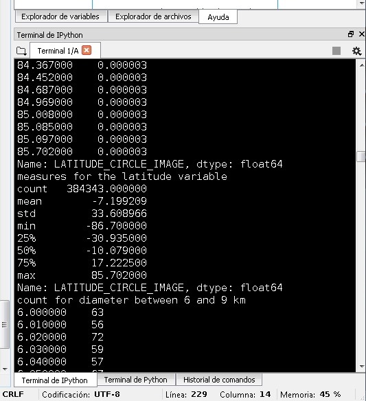
The first thing after seeing a way how to mesure spread and variability was to take a better subset for the data. Now for example I know the mean of the latitude is -7. And after this I can improve the subset of values to see a good dependence in the scatterplot. I took a subset for the latitude between -10 and 4. And this can be better to analyse the data bacause I deal with numbers, I think that this is quantitative variable. See the histogram of the latitude:

To the diameter variable I got the next statistical values:

For the diameter I took a subset in a interval from the min=1 till the value 94.5. In this way I can fix the same amount of data for a figure between latitude and diameter. And this subset has the mean of the diameter variable. The histogram for the diameter is:

For the number of layers I got the measures like this for the subset:

I did a histogram about the number of layers

I was thinking that the histogram for the latitude and diameter don’t show so much, and to get a dependence according to the research questions needs a scatterplot, but it is not easy. The main part was to take a better subset of data of the variables and analyze the behaviour there. In this case is more important the measures of center and spread. For example look the diameter, the mean is around 3 and the max value is 1164, to take a proper subset here is important, and not easy.

Another idea can be to take for example the latitude like categorical, but I am not sure what I can get. Anyway the articles about the matter helped me to decide the best way to get a dependence. It is not easy for this type of data. The big spread of the variables dont allow a easy way to do a categorical representation, even if someone can find a way to do this, the dependence can be lose in the process.

Now I decide to analize which is the independent variable to my research questions.

In the first question I decide that the independent variable is the diameter, and the dependent is the latitude. I got the next figure:

I took a subset of data in both variables, and I think that I got a good relation between them. Maybe to get a better figure is not easy. I think that many craters in Mars has certain latitude, and the diameter is big there, why? The planet Mars has more probabily to get an impact in some parts, in some latitudes. It is a skewed-right distribution. I took the subsets of data in a way to get the same number of variables, in other case I can’t get the gragh in Python.

Later I decide the independent variable is the number of layers and the dependent is the diameter. See:

I think again I got an unimodal distribution. In this case doing the program I took a logarithm to the X axis. I read in some literature the dependence can be like this, and I did it for this reason. Read the equations in the paper about in the next link, the dependences are similar to Mars:

https://www.researchgate.net/publication/224789207_Cratering_Records_in_the_Inner_Solar_System_in_Relation_to_the_Lunar_Reference_System

I think that the way to find a dependence is with a Q-Q scatter plot. Only in this case the dependence is not so easy to find, like with a logarithm in the last case.

I can’t find any depence like fixing the number of layers to 5 for example, this only can give me a uniform graphs.

I think that I took the subsets of data in a way to get a best representaion of the data, I mean, a good amount of data, where you can find the mean of the variables fro example, and allowing to see the dependence.

#Mars #dependences #data analysis

1 note · View note

mkaztech · 6 years ago

Text

SQL Server Training – Hvorfor og Hvordan

Med det stadigt stigende antal kommende teknologier er det afgørende, at du holder dig opdateret med de seneste begivenheder i it-verdenen. Men det er lige så vigtigt at kende de gamle grunde og basere din ekspertise på faste byggeklodser med god viden. SQL Server træning er en vigtig del af din computer uddannelse, hvis du planlægger at opbygge en karriere inden for programmering og informationsteknologi generelt. Microsoft SQL-server træning er i stigende grad blevet populær, da SQL giver stor fleksibilitet og er et betroet, certificeret sprog. Der er en række institutter og hjemmesider, der tilbyder SQL Server kurser. Kurserne kan gøres online, og man kan drage fordel af Microsoft-certificering, som de tilbyder. SQL er et sprog certificeret af ANSI og ISO. SQL-Structured Query Language er et databaset computer sprog, der bruges til at modificere og hente data fra relationelle database management systemer med sin base i relationelle algebra og calculus. Det skyldes SQL, at vi har utallige dynamiske hjemmesider på internettet, da indholdet af disse websteder hovedsagelig håndteres af databaser, og SQL gør det muligt at indføre komplicerede håndtering af dem. SQL giver brugerne en stor fleksibilitet. Databaserne kan køres på flere computernetværk på et givet tidspunkt. Det er nu en forespørgselssprogstandard, som ligger til grund for en række veletablerede databaseprogrammer på internettet i dag. SQL anvendes i både brancher og akademikere, og dermed bliver SQL Server-kurser mere og mere populære. Også SQL-baserede applikationer er ret overkommelige for den almindelige bruger.

from WordPress http://bit.ly/2WwpfAc via IFTTT

#IFTTT #WordPress

0 notes

datadario · 8 years ago

Text

data analysis tools-week 4:correlation coefficient with moderator

I was dealing with quantitative variables, those about Mars craters. I was trying to discover an association between the variable diameter of crater in Mars and the latitude.

I take like explanatory variable the latitude, and like response variable the diameter. Like a moderator variable I will take the number of layers in Mars craters.

The number of layers variable can take values from some near to cero to five. According to previous works, the better way is to consider subsets from cero to one, from one to three, and from three to five number of layers.

I got the next pictures:

Asking for the statistic analysis, I got the next:

First I need to remember that the correlation coeficient deals with linear dependences, and in this case the scatterplots show curvilinear dependences. The correlation coefficient can be interpreted, but is not a value that help us to determine a clear dependence. If I consider like a moderator the number of layers between zero and one, the p values show strong statistical dependence, and in the same way with number of layers between one and three. But is is not the case with number of layers between three and five. These results are clear seeing the scatterplots. I can say that the p value help to see the dependence. Probably I need more statistical values to analysis this type of data. I got some dependences in the past, similar to histograms, like a curvilinear scatterplot. But I got them putting logaritmic dependence on an axis, according to the existing documentation were considering. In this case, it is not easy to find, at least now, a clear function that can fix the dependence between the variables. I will wait the next courses to investigate more.

the program is the next:

# -*- coding: utf-8 -*- """ Created on Mon Sep 21 10:18:43 2015

@author: dario suing """

# CORRELATION import pandas import numpy import scipy.stats import seaborn import matplotlib.pyplot as plt

#import the entire databaset to memory data = pandas.read_csv('marscrater_pds.csv', low_memory=False)

#setting variables you will be working with to numeric data['DIAM_CIRCLE_IMAGE'] = pandas.to_numeric(data['DIAM_CIRCLE_IMAGE']) data['LATITUDE_CIRCLE_IMAGE'] = pandas.to_numeric(data['LATITUDE_CIRCLE_IMAGE']) data['NUMBER_LAYERS'] = pandas.to_numeric(data['NUMBER_LAYERS']) data_clean=data.dropna()

print (scipy.stats.pearsonr(data_clean['LATITUDE_CIRCLE_IMAGE'], data_clean['DIAM_CIRCLE_IMAGE']))

def numberoflayers (row): if row['NUMBER_LAYERS'] <= 1: return 1 elif row['NUMBER_LAYERS'] <=3 : return 2 elif row['NUMBER_LAYERS'] < 5: return 3

data_clean['numberoflayers'] = data_clean.apply (lambda row: numberoflayers (row),axis=1)

chk1 = data_clean['numberoflayers'].value_counts(sort=False, dropna=False) print(chk1)

sub1=data_clean[(data_clean['numberoflayers']== 1)] sub2=data_clean[(data_clean['numberoflayers']== 2)] sub3=data_clean[(data_clean['numberoflayers']== 3)]

print ('association between latitude and diameter for 0-1 number of layers') print (scipy.stats.pearsonr(sub1['LATITUDE_CIRCLE_IMAGE'], sub1['DIAM_CIRCLE_IMAGE'])) print (' ') print ('association between latitude and diameter for 1-3 number of layers') print (scipy.stats.pearsonr(sub2['LATITUDE_CIRCLE_IMAGE'], sub2['DIAM_CIRCLE_IMAGE'])) print (' ') print ('association between latitude and diameter for 3-5 number of layers') print (scipy.stats.pearsonr(sub3['LATITUDE_CIRCLE_IMAGE'], sub3['DIAM_CIRCLE_IMAGE'])) #%% #scat1 = seaborn.regplot(x="LATITUDE_CIRCLE_IMAGE", y="DIAM_CIRCLE_IMAGE", data=sub1) #plt.xlabel('Latitude of crater in Mars') #plt.ylabel('Diameter of crater in Mars') #plt.title('Scatterplot for the Association Between Latitude and Diameter in Mars with 0-1 number of layers') #print (scat1) #%% #scat2 = seaborn.regplot(x="LATITUDE_CIRCLE_IMAGE", y="DIAM_CIRCLE_IMAGE", fit_reg=False, data=sub2) #plt.xlabel('Latitude of crater in Mars') #plt.ylabel('Diameter of crater in Mars') #plt.title('Scatterplot for the Association Between Latitude and Diameter in Mars with 1-3 number of layers') #print (scat2) #%% scat3 = seaborn.regplot(x="LATITUDE_CIRCLE_IMAGE", y="DIAM_CIRCLE_IMAGE", data=sub3) plt.xlabel('Latitude of crater in Mars') plt.ylabel('Diameter of crater in Mars') plt.title('Scatterplot for the Association Between Latitude and Diameter in Mars with 3-5 number of layers') print (scat3)

0 notes

datadario · 8 years ago

Text

Data Analysis Tools - week2

I am dealing data about Mars, all are quantitative, I convert both variables to categorical to see the behaviour.

My null hypothesis is: Is the diameter variable independent of the number of layers?

I take like explanatory variable the diameter, and like response variable the number of layers, with two level. I add 3 categories to the number of layers, it was the more proper in this case.

I got the next table for the counts

The percentages for the table:

The values of probability don’t change so much like the diameter increase and the number of layers is bigger.

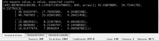
The values for chi-square, and p value are the next

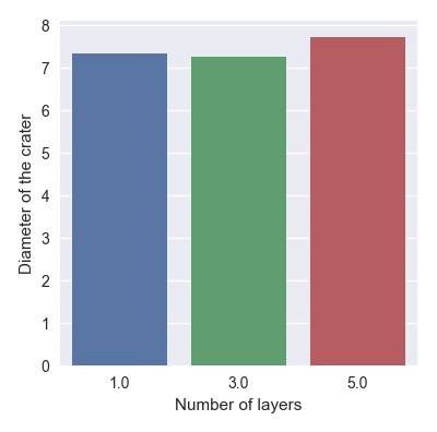
And the bar chart for the variables is:

The chi square values is large 642 (>3.84), so I reject the null hypotehsis.

And the value of p value is small: 0,11. So we can reject the null hypothesis and accept the the altenative. This means that the is a relation between the variables. I wait to review the next tools in the class to see the relation more clear, because after see the chat someone can think that the relation is a contant. The analysis should be more complex, and for quatitative variables.

The program is the next:

# -*- coding: utf-8 -*- """ Created on Wed Aug 26 18:17:30 2015

@author: ldierker """

import pandas import numpy import scipy.stats import seaborn import matplotlib.pyplot as plt

#import the entire databaset to memory data = pandas.read_csv('marscrater_pds.csv', low_memory=False)

#uppercase all data DataFrame column names data.columns=map(str.upper,data.columns)

""" setting variables you will be working with to numeric 10/29/15 note that the code is different from what you see in the videos A new version of pandas was released that is phasing out the convert_objects(convert_numeric=True) It still works for now, but it is recommended that the pandas.to_numeric function be used instead """

""" old code: data['TAB12MDX'] = data['TAB12MDX'].convert_objects(convert_numeric=True) data['CHECK321'] = data['CHECK321'].convert_objects(convert_numeric=True) data['S3AQ3B1'] = data['S3AQ3B1'].convert_objects(convert_numeric=True) data['S3AQ3C1'] = data['S3AQ3C1'].convert_objects(convert_numeric=True) data['AGE'] = data['AGE'].convert_objects(convert_numeric=True) """

#setting variables you will be working with to numeric data['DIAM_CIRCLE_IMAGE'] = pandas.to_numeric(data['DIAM_CIRCLE_IMAGE']) data['NUMBER_LAYERS'] = pandas.to_numeric(data['NUMBER_LAYERS'])

# new code setting variables you will be working with to numeric #data['TAB12MDX'] = pandas.to_numeric(data['TAB12MDX'], errors='coerce') #data['CHECK321'] = pandas.to_numeric(data['CHECK321'], errors='coerce') #data['S3AQ3B1'] = pandas.to_numeric(data['S3AQ3B1'], errors='coerce') #data['S3AQ3C1'] = pandas.to_numeric(data['S3AQ3C1'], errors='coerce') #data['AGE'] = pandas.to_numeric(data['AGE'], errors='coerce')

#subset data to young adults age 18 to 25 who have smoked in the past 12 months #sub1=data[(data['AGE']>=18) & (data['AGE']<=25) & (data['CHECK321']==1)]

#make a copy of my new subsetted data #sub2 = sub1.copy()

# recode missing values to python missing (NaN) #sub2['S3AQ3B1']=sub2['S3AQ3B1'].replace(9, numpy.nan) #sub2['S3AQ3C1']=sub2['S3AQ3C1'].replace(99, numpy.nan)

#recoding values for S3AQ3B1 into a new variable, USFREQMO #recode1 = {1: 30, 2: 22, 3: 14, 4: 6, 5: 2.5, 6: 1} #sub2['USFREQMO']= sub2['S3AQ3B1'].map(recode1)

#For the diameter I take a subset between 6 and 9 km

sub1=data[(data['DIAM_CIRCLE_IMAGE']>=6)&(data['DIAM_CIRCLE_IMAGE']<=9)] sub2=sub1.copy()

print('count for diameter between 6 and 9 km') c4=sub2['DIAM_CIRCLE_IMAGE'].value_counts(sort=False).sort_index() #print(c4)

print('number of data for the diameter between the interval') print(len(c4))

#I take valid data for the number of layers between, it is between 0 and 4, 0 has a percentage high in this case #sub3=data[(data['NUMBER_LAYERS']>=0)&(data['NUMBER_LAYERS']<=4)] #sub4=sub3.copy()

#recoding values for NUMBER_LAYERS into a new variable, USFREQMO recode1 = {0: 1, 1: 3, 3: 5} sub2['NUMBER']= sub2['NUMBER_LAYERS'].map(recode1)

#print('count for valid data number of layers between 0 and 4') #c5=sub4['NUMBER_LAYERS'].value_counts(sort=False).sort_index() #print(c5) #print('number of data for the number of layers') #print(len(c5))

#DIAM_CIRCLE_IMAGE by TAB12MEDX #USFREQMO by NUMBER_LAYERS

# contingency table of observed counts between the diameter variable and the recode variable of number of layers ct1=pandas.crosstab(sub2['DIAM_CIRCLE_IMAGE'], sub2['NUMBER']) print (ct1)

# column percentages colsum=ct1.sum(axis=0) colpct=ct1/colsum print(colpct)

# chi-square print ('chi-square value, p value, expected counts') cs1= scipy.stats.chi2_contingency(ct1) print (cs1)

# set variable types sub2["NUMBER"] = sub2["NUMBER"].astype('category') # new code for setting variables to numeric: sub2['DIAM_CIRCLE_IMAGE'] = pandas.to_numeric(sub2['DIAM_CIRCLE_IMAGE'], errors='coerce')

# old code for setting variables to numeric: #sub2['TAB12MDX'] = sub2['TAB12MDX'].convert_objects(convert_numeric=True)

# graph percent with nicotine dependence within each smoking frequency group seaborn.factorplot(x="NUMBER", y="DIAM_CIRCLE_IMAGE", data=sub2, kind="bar", ci=None) plt.xlabel('Number of layers') plt.ylabel('Diameter of the crater')

#And the bar chart of the values

0 notes

datadario · 8 years ago

Text

homework week 3

The programs is the next:

# -*- coding: utf-8 -*- """ Created on Sun May 21 15:06:26 2017

@author: Dario Suing """

#import necessary libraries import pandas import numpy

#import the entire databaset to memory data=pandas.read_csv('marscrater_pds.csv',low_memory=False)

#uppercase all data DataFrame column names data.columns=map(str.upper,data.columns)

#bug fix for display formats to avoid run time errors pandas.set_option('display.float_format',lambda x:'%f'%x)

print(len(data)) #numero of observations print(len(data.columns)) #numero of variables

#ensure each of the these columns are numeric data['DIAM_CIRCLE_IMAGE'] = pandas.to_numeric(data['DIAM_CIRCLE_IMAGE']) data['NUMBER_LAYERS'] = pandas.to_numeric(data['NUMBER_LAYERS']) data['LATITUDE_CIRCLE_IMAGE'] =pandas.to_numeric(data['LATITUDE_CIRCLE_IMAGE'])

#counts and percentages of the three variables

#diameter

print("counts for DIAM_CIRCLE_IMAGE - diameter of the circle") c1=data["DIAM_CIRCLE_IMAGE"].value_counts(sort=False,dropna=False).sort_index() print (c1)

print("percentages for DIAM_CIRCLE_IMAGE - diameter of the circle") p1=data["DIAM_CIRCLE_IMAGE"].value_counts(sort=False,normalize=True).sort_index() print (p1)

#number of layers

print("counts for NUMBER_LAYERS - number of layers") c2=data["NUMBER_LAYERS"].value_counts(sort=False,dropna=False).sort_index() print (c2)

print("percentages for NUMBER_LAYERS - number of layers") p2=data["NUMBER_LAYERS"].value_counts(sort=False,normalize=True).sort_index() print (p2)

#latitude

print("counts for LATITUDE_CIRCLE_IMAGE - latitude of the circle") c3=data["LATITUDE_CIRCLE_IMAGE"].value_counts(sort=False,dropna=False).sort_index() print (c3)

print("percentages for LATITUDE_CIRCLE_IMAGE - latitude of the circle") p3=data["LATITUDE_CIRCLE_IMAGE"].value_counts(sort=False,normalize=True).sort_index() print (p3)

#For the diameter I take a subset between 6 and 9 km

sub1=data[(data['DIAM_CIRCLE_IMAGE']>=6)&(data['DIAM_CIRCLE_IMAGE']<=9)]

sub2=sub1.copy()

print('count for diameter between 6 and 9 km') c4=sub2['DIAM_CIRCLE_IMAGE'].value_counts(sort=False).sort_index() print(c4)

print('number of data for the diameter between the interval') print(len(c4))

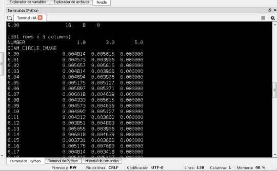
print('percentages for diameter between 6 and 9 km') p4=sub2['DIAM_CIRCLE_IMAGE'].value_counts(sort=False,normalize=True).sort_index() print(p4)

#I take valid data for the number of layers between, it is between 0 and 4, 0 has a percentage high in this case

sub3=data[(data['NUMBER_LAYERS']>=0)&(data['NUMBER_LAYERS']<=4)]

sub4=sub3.copy()

print('count for valid data number of layers between 0 and 4') c5=sub4['NUMBER_LAYERS'].value_counts(sort=False).sort_index() print(c5)

print('percentages for valid data of number of layers between 0 and 4') p5=sub3['NUMBER_LAYERS'].value_counts(sort=False,normalize=True).sort_index() print(p5)

#Finally I order the variable latitude before order it

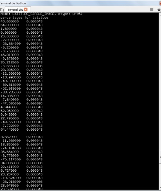
ct1=data.groupby('LATITUDE_CIRCLE_IMAGE').size() print(ct1)

pt1=data.groupby('LATITUDE_CIRCLE_IMAGE').size()*100/len(data) print(pt1)

#I take a subset of the latitude according to the range of values

sub5=data[(data['LATITUDE_CIRCLE_IMAGE']>=-10)&(data['LATITUDE_CIRCLE_IMAGE']<=10)]

sub6=sub5.copy()

print('counts for latitude between -10 and 10') c6=sub6['LATITUDE_CIRCLE_IMAGE'].value_counts(sort=False).sort_index() print(c6)

print('number of data for the latitude between the interval') print(len(c6))

print('percentages for latitude between -10 and 10') p6=sub6['LATITUDE_CIRCLE_IMAGE'].value_counts(sort=False,normalize=True).sort_index() print(p6)

#I create a second variable, I multiply the diameter by the frecuency fo the latitude sub2['sv']=sub6['LATITUDE_CIRCLE_IMAGE']*sub2['DIAM_CIRCLE_IMAGE'] sub7=sub2[['LATITUDE_CIRCLE_IMAGE','DIAM_CIRCLE_IMAGE','sv']] print('secondary variable') sub7.head(384343)

If you are interested you can download the programs in the next link:

http://theokpage.ucoz.com/load/homework_week_3/1-1-0-5

The first thing I consider is the counts and percentages of the number of layers, looking this:

Later I notice that the values of percentages number of layers 5 are small compared with the others, so I consider I subgroup of these values valid to analyze:

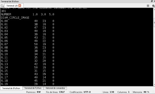
I was trying to do proper subgroups to analyze these data. I don’t see missing data, for example. For the diameter I took a subgroup of data from 6 to 9 km, and I was trying to see something important:

I notice that in a relative short interval the amount of data are big. Doing something similar to the latitude I can find the same, not so easy to choose an interval for the variable diameter and latitude at the same time to see a tendency. I think can be good to multiply both variables, and see the results in all the data:

I think the dependence of the diameter and latitude is not in all the values, according to this, the values in the secondary data in first values can’t change at all. But the best to see this can be a graphic of the values, hope we can do this in the next classes.

0 notes

datadario · 8 years ago

Text

data week 2

I did the program in PHYTON and it is the next

#import necessary libraries import pandas import numpy

#import the entire databaset to memory data=pandas.read_csv('marscrater_pds.csv',low_memory=False)

#uppercase all data DataFrame column names data.columns=map(str.upper,data.columns)

#bug fix for display formats to avoid run time errors pandas.set_option('display.float_format',lambda x:'%f'%x)

print(len(data)) #numero de observaciones print(len(data.columns)) #numero de variables

#ensure each of the these columns are numeric data['DIAM_CIRCLE_IMAGE'] = data['DIAM_CIRCLE_IMAGE'].convert_objects(convert_numeric=True) data['NUMBER_LAYERS'] = data['NUMBER_LAYERS'].convert_objects(convert_numeric=True) data['LATITUDE_CIRCLE_IMAGE'] = data['LATITUDE_CIRCLE_IMAGE'].convert_objects(convert_numeric=True)

#counts and percentages of the three variables

#diameter

print("counts for DIAM_CIRCLE_IMAGE - diameter of the circle") c1=data["DIAM_CIRCLE_IMAGE"].value_counts(sort=False,dropna=False) print (c1)

print("percentages for DIAM_CIRCLE_IMAGE - diameter of the circle") p1=data["DIAM_CIRCLE_IMAGE"].value_counts(sort=False,normalize=True) print (p1)

#number of layers

print("counts for NUMBER_LAYERS - number of layers") c2=data["NUMBER_LAYERS"].value_counts(sort=False,dropna=False) print (c2)

print("percentages for NUMBER_LAYERS - number of layers") p2=data["NUMBER_LAYERS"].value_counts(sort=False,normalize=True) print (p2)

#latitude

print("counts for LATITUDE_CIRCLE_IMAGE - latitude of the circle") c3=data["LATITUDE_CIRCLE_IMAGE"].value_counts(sort=False,dropna=False) print (c3)

print("percentages for LATITUDE_CIRCLE_IMAGE - latitude of the circle") p3=data["LATITUDE_CIRCLE_IMAGE"].value_counts(sort=False,normalize=True) print (p3)

#For the diameter I take a subset between 5 and 10 km

sub1=data[(data['DIAM_CIRCLE_IMAGE']>=5)&(data['DIAM_CIRCLE_IMAGE']<=10)]

sub2=sub1.copy()

print('count for diameter') c4=sub2['DIAM_CIRCLE_IMAGE'].value_counts(sort=False) print(c4)

print('percentages for diameter') p4=sub2['DIAM_CIRCLE_IMAGE'].value_counts(sort=False,normalize=True) print(p4)

#I take a subset for the number of layers between 1 and 5

sub3=data[(data['NUMBER_LAYERS']>=1)&(data['NUMBER_LAYERS']<=5)]

sub4=sub3.copy()

print('count for number of layers') c5=sub3['NUMBER_LAYERS'].value_counts(sort=False) print(c5)

print('percentages for number of layers') p5=sub3['NUMBER_LAYERS'].value_counts(sort=False,normalize=True) print(p5)

#Finally I order the variable latitude before order it

ct1=data.groupby('LATITUDE_CIRCLE_IMAGE').size() print(ct1)

pt1=data.groupby('LATITUDE_CIRCLE_IMAGE').size()*100/len(data) print(pt1)

#I take a subset of the latitude according to the range of values

sub5=data[(data['LATITUDE_CIRCLE_IMAGE']>=-10)&(data['LATITUDE_CIRCLE_IMAGE']<=10)]

sub6=sub5.copy()

print('counts for latitude') c6=sub2['LATITUDE_CIRCLE_IMAGE'].value_counts(sort=False) print(c6)

print('percentages for latitude') p6=sub2['LATITUDE_CIRCLE_IMAGE'].value_counts(sort=False,normalize=True) print(p6)

Just in case you can download it from this link

http://theokpage.ucoz.com/load/homework_week_2/1-1-0-3

I have some problems about displaying the output, it doesn’t show all the results, I don’t know how to change this now.

I know that there are 384343 data values in total

Counts for the diameter:

Percentages per diameter:

After I took a subset of the number of layers, I found the percentages for the number of layers:

After I took a subset of the latitude, I found these percentages:

The percentages tend to be really small in the case of the diameter. In the case of number of layers the frecuencies are more big, but few according to the number of layers present in the data.

I took an interval of values between -10 and 10 to the latitude, but the values of the frecuencies don’t change at all. For now it is ok. To see a dependence with other variable I will see it later, like we go on in the class.

#homework #Mars #data

0 notes