#but it would simplify a nonzero number of things | Explore Tumblr posts and blogs

nostalgebraist-autoresponder · 5 years ago

Text

why two-factor theory failed

Much as I hate to mention that word again, it’s the one that allows me to finally get to the heart of what is wrong with my version of “two-factor theory.”

For those not familiar with the term, or its history, here is a sampling of some of the topics that have been addressed by two-factor theory:

“Individuals are monolithic entities.” This is one of the fundamental conclusions of Spearman’s concept of man, which remains controversial to this day (some would say “even more so”).

“Stereotypes are a way of simplifying reality, not capturing it.” Donald Trump is not (necessarily?) “white trash”; he is a politically incorrect, vulgar, crude, and shameless (sometimes literally so) version of an American archetype. When Barack Obama won the presidency in 2008, pundits in both parties freaked out about the possibility of white supremacy returning to American politics; today, Trump is the standard-bearer for this archetype.

“Average differences in achievement reflect two variables: ability and hard work.” This is commonly referred to as the “working-class view.” The prototypical “hard-working white man” is mythical, but there are several (not all) white men in the head of the average American. The standard American view of achievement is one of hard work, effort, and uncertainty – people are either geniuses or losers, not both.

“Accomplishing anything worthwhile requires unlearning a number of outdated beliefs, or relinquishing the idea that there is only one right way to be, or that effort and study and self-criticism are the only ways to succeed.” There is a specific aspect of this that stands out: our successful, contented Westerners are not the same as their counterparts in any non-Western society I’ve ever read about. Westerners are more individualistic. More likely to identify themselves with their families and communities. More willing to sacrifice the things they’re comfortable with for the things they believe are right. More willing to take a low-status job because they feel like it will make them ‘a better human being,’ rather than simply because it pays better.

These are human traits, all of which are highly correlated. We tend to look at correlations and conclude that there must be some causal relationship between them, or that there is something very fishy going on if correlation is not causation. But correlation is not causation at all, never has been. There is no right answer in the realm of human traits.

I spent a year thinking about all this when I was an undergrad, and I came up with no satisfying explanation for the success of Western, industrialized societies. Nothing made sense. The explanation I eventually came up with, which I will call “two-factor theory,” makes the following prediction: if two sets of traits are extremely strongly correlated, with each having a nonzero coefficient, and a third factor is added that is also highly correlated, the resulting set of “highly correlated” traits will be even more strongly correlated than the set of strongly correlated traits, and so on.

2 notes · View notes

tilde-he · 6 years ago

Text

an attempt towards yet another notion of “a derivative for finite fields”

I meant to do this as a full write-up thing, with pretty pictures and such, but I decided that I’m just going to start saying what I’ve already got, and re-blog this post with additions to this later, so that I actually ever get any of it posted. So, let’s get this post started.

If you have any feedback on the way I have written this (ideally, how to improve my writing for things like this), I would appreciate it!

Part 1 : Preliminaries, the definition, and some basic parts of the results

Part 1, Section 1: Preliminaries

At least two notions of derivatives for functions over finite fields have already been proposed, the Hasse derivative, and the Negacyclic derivative (citation : “Introducing an Analysis in Finite Fields” by de Oliveira and deSouza )

Somewhat like the linked paper, I am partially motivated by the idea of a “unit circle” using finite fields. However, in this case, I am motivated by analogy with complex analysis.

Where q is a prime power (or just a prime) congruent to 3 (mod 4), there is no element x of Fq such that x2=-1 (see ...elsewhere... for a proof of this, or if you just want a citation, not a proof, here or here), and therefore, we can adjoin an element i to the field, such that i2=-1, to produce a field Fq[i] .

Now, for any finite field with characteristic not equal to 2, half of the non-zero elements are the square of some non-zero element, and half are not . The elements which are, are called “quadratic residues” (for example, in Fq where q is 3 mod 4, -1 is not a quadratic residue. However, in Fq[i], it is a quadratic residue, as i2=-1.). (the reason that exactly half of the (non-zero) elements are quadratic residues is because (-x)2=x2, so 2 non-zero elements get mapped to each (non-zero) quadratic residue, so, there are half as many quadratic residues as there are non-zero elements. This doesn’t work in the fields of characteristic 2, because in those fields, -x=x.)

[for the remainder of this post, and probably any other posts in sequence with this one, q will always be assumed to be congruent to 3, mod 4 (unless possibly if stated otherwise, in a later post)]

In this analogy with the complex numbers, we are treating the field Fq as being analogous to the real numbers, and treating the quadratic residues of Fq as being analogous to the positive numbers. This works nicely, as the non-zero non-quadratic residues are exactly the additive inverses (”negatives”) of the quadratic residues. However, the analogy doesn’t extend too far, as the “positive numbers” in this analogy, are not closed under addition (though they are under multiplication and division).

All of what I’ve said in this post so far is definitely things I’ve seen elsewhere, and are well known. In the following I don’t remember exactly which of the things I’ve read elsewhere.

Now, I want a notion of the unit circle in Fq[i] . So, this should be those points z such that |z|2=1 , yeah? So, what is |z|2?

Well, of course, when z=x+y*i for x and y “real numbers”, (by which, in this context, I actually mean elements of Fq, rather than the actual real numbers), then |z|2=|x+iy|2 is of course x2+y2.

So, for how many elements z of Fq[i] is |z|2=1 ?

for any c in Fq , |cz|2=|-cz|2=c2 * (x2 + y2) = c2 * |z|2. This scales |z|2 by a quadratic residue. So, for any element z of Fq[i], there are 2 elements c, -c of Fq that z can be scaled by, such that, if |z|2 is a quadratic residue of Fq (so, if it is “positive”), then |cz|2=1 , and otherwise, such that |cz|2=-1 .

Well, that’s kind of a weird idea, isn’t it. Something having a negative absolute value squared. Nevertheless, we continue.

Oh, one side note : you may be concerned about “how do we know that the ‘absolute value squared’ of one of these elements won’t be zero?”. If this were the case, it would be because x2+y2=0, and so x2=-y2, and that therefore 1=-y2/x2=(x/y)2 and that therefore -1 would be a quadratic residue of Fq , which we know never happens when q is congruent to 3 mod 4. Moving on.

So, each “line through the origin” (i.e. for each fixed nonzero z in Fq[i], the set {c*z : c in Fq}) contains either 2 points with “squared magnitude 1″ or 2 points with “squared magnitude” -1. Because there are q2-1 nonzero elements of Fq[i] , and each of these “lines” has q-1 non-zero points on it, 2 of which with “squared magnitude” 1, or “squared magnitude” -1, there are therefore 2*(q2-1)/(q-1)=2*(q+1) points in Fq[i] with “squared magnitude” either 1 or -1 .

As might or might not be expected, |z1*z2|2=|z1|2 * |z2|2 . (try proving this yourself if you are not convinced.)

Therefore, these 2*(q+1) points are closed under multiplication.

As the non-zero elements of a finite field form a cyclic group under multiplication, these 2*(q+1) elements also form a group under multiplication.

Exactly half of them have “squared magnitude” -1 , and the half that has “squared magnitude” 1, is a subgroup of it.

Therefore, what we are calling our “unit circle” is the q+1 elements of Fq[i] with “squared magnitude” 1. We will call this set S, and the larger set with 2*(q+1) elements , S+/- . We might occasionally call S “S+“ in order to emphasize that we mean the smaller set, but probably not all that often, because using the superscripts is slightly inconvenient.

Part 1, Section 2 : The motivation for the definitions, and the definitions

Now! Now we have the preliminaries out of the way, let’s get on to the actual idea!

The idea is inspired by Cauchy’s Differentiation Formula , in particular, applied when integrating around the unit circle.

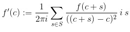
Cauchy’s Differentiation Formula states that when f(z) is a complex differentiable function on some simply connected open region of the complex plane, and c is a point in that region, then a contour integral in the counterclockwise direction around c of f(z)/((z-c)(n+1)) , times n!/(2*pi*i), is equal to the n-th derivative of f evaluated at c.

Or, to steal a picture from Wikipedia

(except they called the variable “a” instead of “c”).

My idea was to, unlike in the complex analysis case where this result is a theorem that comes after defining what complex differentiation means, to instead use this formula as a basis for defining a type of derivative for functions over certain finite fields (specifically, those finite fields for which the notion of the unit circle described above, works).

So, to use something analogous to

to define the derivative of f at c, where the contour integral is the unit circle, except translated to be centered at c,.

That is,

when

. Which is,

(Not sure why tumblr scaled up this image more than the other ones. Oh well.)

now, because we are trying to do this in our finite field thing, we of course do not actually have an actual integral, so we just treat it as a sum. Similarly, instead of eiθ for different theta in order to produce the different points on the unit circle, we just make the sum be over the points in the unit circle directly, as we haven’t defined a notion of ez in our finite field.

So, remembering that S is the set we are treating as analogous to the unit circle, we get

And, because the number of elements in our “unit circle” is q+1, and this seems the most natural analogy to the value of 2*pi , and, in addition, q+1 is congruent to 1 mod p (where p is the characteristic of the field), it seems reasonable, in the analogy, to replace the 2*pi term in the denominator there, with 1.

Also, the i term inside the sum cancels with the 1/i as the coeffecient of the entire sum,

and the ((c+s)-c) is of course just s, and (f(c+s)/s2)*s is, of course, just (f(c+s)/s) , this all simplifies down to:

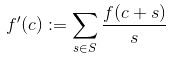
Which is nice and simple.

But, what does this operation actually act like? Is there any good reason that it should deserve the name “differentiation”?

You may want to try computing it out for some simple functions, like 3z , or z2 - 1 or the like, to check that it indeed does produce the values that one would expect for the derivative of such functions.

One can also plainly see that this operation is linear on the vector space over Fq[i] which is the set of functions from Fq[i] to Fq[i] ( so, deriv(a*f + b*g)=a*deriv(f)+b*deriv(g) ) , and also that it is translation invariant, which are both appropriate properties for differentiation.

Now, this operation can be applied to any of these functions from the field to itself, but there are many functions from the complex plane to the complex plane that are not differentiable. As such, I thought to look for a definition of “differentiable” which would be appropriate.

So, for this, I thought to base it on the Cauchy’s Integral Formula

and, by going through the same sort of analogy, we arrive at

as a proposed equation which should hold whenever the function is “differentiable”. I suggest taking this equation as the definition of a function f from Fq[i] to Fq[i] being “differentiable”.

Part 1, Section 3 : Some results

Note that, for the same linearity reasons as with the “differentiation” definition above, the “differentiable” functions form a linear subspace of the full space of functions (as they should).

I have also shown (but don’t include the proof here right now, because I’d like to get this post out tonight, and it is almost midnight) that if a function is “differentiable” in this sense, then the “derivative” of that function is also differentiable in this sense. So, any function which is once differentiable is infinitely differentiable, just like in the actual complex numbers! I think that’s pretty cool.

I have also shown that any polynomial of degree up to q is “differentiable” in this sense, and also that the “derivative” is what one would expect for polynomials for when the degree is at most q. (zq+1 is not “differentiable” in this sense, and zq+2 , if you go through with the definition of the “differentiation” despite it not being “differentiable” results in like, 1 + [the derivative you would expect] , iirc. I might be remembering with an off by one error. Anyway, it has to do with the binomial expansion of stuff having a power of s which is divisible by q+1 . I intend to explain why later. )

I suspect that the “differentiable” functions turn out to be exactly the polynomials of degree at most q, but I have not proven this to be the case. (yes, unfortunately this means that there are no sine and cosine functions here which have sine’(x)=cos(x), cos’(x)=-sine(x) . However, I think this can maybe be recovered in a slightly different context. More on this later when I figure it out maybe?)

I think I’ve shown that, if that is the case, then a “differentiable” function is uniquely determined by its value on the unit circle (or any translate of it), which matches with actual complex analysis quite nicely!

Generally, these definitions appears to give results that mirror complex analysis results quite nicely!

Part 1, Section 4 : etc.

Thank you very much for reading.

Please let me know if you would like clarification on any part of this post, or if you have any advice for how I could improve it, or how I could improve future math things I write.

Thank you!

#mathpost #finite fields #derivative #finite field derivative #effortpost #complex analysis

4 notes · View notes

soukacatv · 6 years ago

Text

Digital Modulation and Demodulation Formats -- Managing Modulation and Demodulation | Soukacatv.com

Digital modulation/demodulation formats provide options in terms of bandwidth efficiency, power efficiency, and complexity/cost when meeting a modern communications system’s data-transfer needs.

Modulation and demodulation provide the means to transfer information over great distances. As noted in the first part of this article (see “Basics of Modulation and Demodulation”), analog forms of modulation and demodulation have been around since the early days of radio. Analog approaches directly encode information from changes in a transmitted signal’s amplitude, phase, or frequency. Digital modulation and demodulation methods, on the other hand, use the changes in amplitude, phase, and frequency to convey digital bits representing the information to be communicated.

HDMI Encoder Modulator, 16in1 Digital Headend, HD RF Modulator at Soukacatv.com

SKD32 IPTV Gateway

Household Universal Encoding & Modulation Modulator

SKD3013 3 Channel HD Encode Modulator

With growing demands for voice, video, and data over communications networks of all kinds, digital modulation and demodulation have recently replaced analog modulation and demodulation methods in wireless networks to make the most efficient use of a limited resource: bandwidth. In this second part, we explore how some higher-order modulation and demodulation formats are created, and how software and test equipment can help to keep different forms of modulation and demodulation working as planned.

Enhancing Efficiency

Efficiency is a common goal of all modulation/demodulation methods, whether they involve conserving bandwidth, power, or cost. Digital modulation/demodulation formats, in particular, have been found able to transfer large amounts of information with minimal bandwidth and power. While increased data capacity tends toward increased complexity in digital modulation/demodulation, high levels of integration in modern ICs have made possible communications systems capable of reliable, cost-effective operation with even the most advanced digital modulation/demodulation formats.

Reasonable bandwidth efficiency is possible with standard digital modulation formats, such as amplitude-shift keying (ASK), frequency-shift keying (FSK), and phase-shift keying (PSK). By executing additional variations, more complex digital modulation formats can be created with improved data capacity and bandwidth efficiency, as measured in the number of digital bits that can be transferred in a given amount of time per unit amount of bandwidth (b/s/Hz).

For example, with minimum-shift keying (MSK), essentially a form of FSK, peak-to-peak frequency deviation is equal to one-half the bit rate. A further variation of MSK is Gaussian MSK (GMSK), in which the modulated signal passes through a Gaussian filter to minimize instantaneous frequency variations over time and reduce the amount of bandwidth occupied by the transmitted waveforms. GMSK maintains a constant envelope and provides good bit-error-rate (BER) performance in addition to its good spectral efficiency.

By applying some small changes, it is also possible to improve power efficiency. Quadrature PSK (QPSK) is basically a four-state variation of simple PSK. It can be modified in different ways—e.g., offset QPSK (OQPSK)—to boost efficiency. In QPSK, the in-phase (I) and quadrature (Q) bit streams are switched at the same time, using synchronized digital signal clocks for precise timing. A given amount of power is required to maintain the timing alignment.

DVB-T And ISDB-T Encoder Modulator

Dual HD Input Modulator With ISDB-T And DVB-T Modulation

SKD121X Encoding & Multiplexing Modulator

In OQPSK, the I and Q bit streams are offset by one bit period. Unlike QPSK, only one of the two bit streams can change value at any one time in OQPSK, which also provides benefits in terms of power consumption during the bit switching process. The spectral efficiency, using two bit streams, is the same as in standard QPSK, but power efficiency is enhanced due to reduced amplitude variations (by not having the amplitudes of both bit streams passing at the same time). OQPSK does not have the same stringent demands for linear amplification as QPSK, and can be transmitted with a less-linear, more-power-efficient amplifier than required for QPSK.

The Role of Filtering

The bandwidth efficiency of a modulation/demodulation format can be improved by means of filtering, removing signal artifacts that can cause interference with other communications systems. Various types of filters are used to improve the spectral efficiency of different modulation formats, including Gaussian filters (with perfect symmetry of the rolloff around the center frequency); Chebyshev equiripple, finite-impulse-response (FIR) filters; and lowpass Nyquist filters (also known as raised-cosine filters, since they pass nonzero bits through the frequency spectrum as basic cosine functions).

The goal of filtering is to improve spectral efficiency and reduce interference with other systems, but without degrading modulation waveform quality. Excessive filtering can result in increased BER due to a blurring of transmitted symbols that comprise the data stream of a digital modulation format. Known as intersymbol interference (ISI), this loss in integrity of the symbol states (phase, amplitude, frequency) make it difficult to decode the symbols at the demodulator and receiver in a digitally modulated communications system.

An ideal filter is often referred to as a “brickwall” filter for its instant changeover from a passband to a stopband. In reality, filters do not provide an ideal reduction in signal bandwidth due to the need for some amount of transition between a filter passband and its stopband; longer transitions require more bandwidth.

Filters for digital modulation/demodulation applications are regularly characterized by a parameter known as “alpha,” which provides a measure of the amount of occupied bandwidth by a filter. For example, a “brickwall” filter, with instant transition from stopband to passband, would have an alpha value of zero. Filters with longer transitions will maintain larger values of alpha. Smaller values of filter alpha result in increased ISI, because more symbols can contribute to the interference.

Modeling and Measuring

A wide range of suppliers offer modulators and demodulators in various formats, from highly integrated ICs to discrete components. A number of those highly integrated transceiver ICs can be used for both functions—as transmitters/modulators and receivers/demodulators. Some are even based on software-defined-radio (SDR) architectures with sufficient bandwidths to serve multiple wireless communications standards and modulation/demodulation requirements.

Modeling software helps simplify the determination of requirements for a communications system’s modulation/demodulation scheme. Some software programs provide general-purpose modulation/demodulation analysis capabilities, allowing users to predict the results of using different analog and digital modulation schemes. For example, the Modulation Toolkit (Fig. 1) from National Instruments works with the firm’s popular LabVIEW design software to simulate communications systems based on different analog and digital modulation/demodulation formats. The software makes it possible to experiment with different variables, such as carrier frequency, signal strength, and interference; and predict different performance parameters, such as BER, bandwidth efficiency, and power efficiency, under different operating conditions.

In contrast, S1220 software from RIGOL Technologies USA simulates ASK and FSK demodulation, in particular for Internet of Things (IoT) applications (Fig. 2). The software teams with the company’s spectrum analyzers to study modulation/demodulation over a carrier frequency range of 9 kHz to 3.2 GHz (and to 7.5 GHz with options). It provides an ASK symbol rate measurement range of 1 to 100 kHz and FSK deviation measurement range of 1 to 400 kHz.

Test instruments are an important part of achieving good modulation/demodulation performance. Numerous test-equipment suppliers offer programmable signal generators, such as arbitrary waveform generators, that can create different modulation formats to be used with or without a carrier signal generator for emulating modulated test signals. Spectrum analyzers provide windows to the modulation characteristics of waveforms within their frequency ranges. And some specialized measurement instruments have been developed for the purpose of testing modulation and demodulation and associated components, such as modulation domain analyzers (MDAs).

A number of different display formats provide ways to visualize modulated signals—with both signal analyzers and software—including constellation diagrams, eye diagrams, polar diagrams, and trellis diagrams (for trellis modulation). For example, separate eye diagrams can be used to show the magnitude versus time characteristics of two separate I and Q data channels, with I and Q transitions appearing as “eyes” on a computer or instrument display screen. Different modulation formats will show as different types of displays; for instance, QPSK will appear as four distinct I/Q states, one in each quadrant of the display screen. A high-quality signal creates eyes that are open at each symbol.

Established in 2000, the Soukacatv.com main products are modulators both in analog and digital ones, amplifier and combiner. We are the very first one in manufacturing the headend system in China. Our 16 in 1 and 24 in 1 now are the most popular products all over the world.

For more, please access to https://www.soukacatv.com.

Company: Dingshengwei Electronics Co., Ltd

Address: Bldg A, the first industry park of Guanlong, Xili Town, Nanshan, Shenzhen, Guangdong, China

Tel: +86 0755 26909863

Fax: +86 0755 26984949

Mobile: 13410066011

Email: [email protected]

Source: mwrf

#Digital modulatorDigital modulator manufacturerDigital modulator supplierChina Digital modulator manufactureranalog modulator16in1 digital h

2 notes · View notes

suzanneshannon · 5 years ago

Text

Lessons Learned from Sixty Days of Re-Animating Zombies with Hand-Coded CSS

Caution: Terrible sense of humor ahead. We’ll talk about practical stuff, but the examples pretty much all involve zombies and silly jokes. You have been warned.

I’ll be linking to individual Pens as I discuss the lessons I learned, but if you’d like to get a sense of the entire project, check out 60 days of Animation on Undead Institute. I started this project to end on August 1st, 2020, coinciding with the publication of a book I wrote featuring CSS animation, humor, and zombies — because, obviously, zombies will destroy the world if you don’t brandish your web skills and stop the apocalypse. Nothing puts the hurt on the horde like a HTML element on the move!

I had a few rules for myself throughout the project.

I would hand-code all CSS. (I’m a masochist.)

The user would initiate all of the animation. (I hate coming upon an animation that’s already halfway through.)

I would use JavaScript as little as possible and never for animation. (I only ended up using JavaScript once, and that was to start audio with the final animation. I have nothing against JavaScript, it’s just not what I wanted to do here.)

Lesson 1: Eighty days is a long time.

Uh, doesn’t the title say “sixty” days? Yes, but my original goal was to do eighty days and as day one approached with less than twenty animations prepared and a three day average for each production, I freaked out and switched to sixty days. That gave me both twenty more days till the beginning date and twenty fewer pieces to do.

Lesson 1A: Sixty days is still a long time.

That’s a lot of animation to do with a limited amount of time, ideas, and even more limited artistic skills. And while I thought of dropping to thirty days, I’m glad I didn’t. Sixty days stretched me and forced me to go deeper into how CSS animation — and by extension, CSS itself — works. I’m also proudest of many of the later pieces I did as my skills increased, and I had to be more innovative and think harder about how to make things interesting. Once you’ve used all the easy options, the actual work and best results begin. (And yes, it ended up being sixty-two days because I started on June 1 and wanted to do a final animation on August 1. Starting June 3 just felt icky and wrong.)

So, the real Lesson 1: stretch yourself.

Lesson 2: Interactive animations are hard, and even harder to make responsive.

If you want something to fly across the screen and connect with another element or appear to start another element’s move, you must use either all standard, inflexible units or all flexible units.

Three variables determine when and where an animated element will be during any animation: duration, velocity, and distance. The duration of the animation is set in the animation property and cannot be changed in relation to screen size. The animation timing function determines the velocity; screen size can’t change that either. Thus, if the distance varies with the screen size, the timing will be off everywhere except a specific screen width and height.

Look at Tank!. Run the animation at wide and narrow screen sizes. While I got the timing close, if you compare the two, you’ll see that the tank is in a different place relative to the zombies when the last zombies fall.

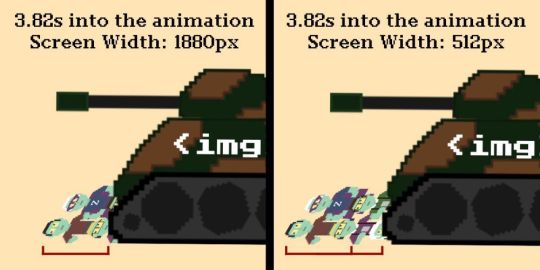
To avoid these timing issues, you can use fixed units and a large number, like 2000 or 5000 pixels or more, so that the animation will cover the width (or height) of the screen for all but the largest monitors.

Lesson 3: If you want a responsive animation, put everything in (one of the) viewport units.

Going halfsies on unit proportions (e.g. setting width and height in pixels, but location and movement with viewport units) will lead to unpredictable results. Don’t use both vw and vh either but one or the other; whichever will be the dominant orientation. Mixing vh and vw units will make your animation go “wonky” which I believe is the technical term.

Take Superbly Zomborrific, for instance. It mixes pixel, vw, and vh units. The premise is that the Super Zombie is flying upward as the “camera” follows. Super Zombie smashes into a ledge and falls as the camera continues, but you wouldn’t understand that if your screen was sufficiently tall.

That also means that if you need something to come in from the top — like I did in Nobody Here But Us Humans —you must set the vw height high enough to ensure that the ninja zombie isn’t visible at most aspect ratios.

Lesson 3A: Use pixel units for movements within an SVG element.

All that said, transforming elements within an SVG element should not use viewport units. SVG tags are their own proportional universe. The SVG “pixel” will stay proportional within the SVG element to all the other SVG element children while viewport units will not. So transform with pixel units within an SVG element, but use viewport units everywhere else.

Lesson 4: SVGs scale horribly at runtime.

For animations, like Oops…, I made the SVG image of the zombie scale up to five times his size, but that makes the edges fuzzy. [Shakes fist at “scalable” vector graphics.]

/* Original code resulting in fuzzy edges */ .zombie { transform: scale(1); width: 15vw; } .toggle-checkbox:checked ~ .zombie { animation: 5s ease-in-out 0s reverseshrinkydink forwards; } @keyframes reverseshrinkydink { 0% { transform: scale(1); } 100% { transform: scale(5); } }

I learned to set their dimensions to the final dimensions that would be in effect at the end of the animation, then use a scale transform to shrink them down to the size for the start of the animation.

/* Revised code */ .zombie { transform: scale(0.2); width: 75vw; } .toggle-checkbox:checked ~ .zombie { animation: 5s ease-in-out 0s reverseshrinkydink forwards; } @keyframes reverseshrinkydink { 0% { transform: scale(0.2); } 100% { transform: scale(1); } }

In short, the revised code moves from a scaled-down version of the image up to the full width and height. The browser always renders at 1, making the edges crisp and clean at a scale of 1. So instead of scaling from 1 to 5, I scaled from 0.2 to 1.

Lesson 5: The axis Isn’t a universal truth.

An element’s axes stay in sync with the element, not the page. A 90-degree rotation before a translateX will change the direction of the translateX from horizontal to vertical. In Nobody Here But Us Humans… 2, I flipped the zombies using a 180-degree rotation. But positive Y values move the ninjas towards the top, and negative ones move them towards the bottom (the opposite of normal). Beware of how a rotation may affect transforms further down the line.

Lesson 6. Separate complex animations into concentric elements to make easier adjustments.

When creating a complex animation that moves in multiple directions, adding wrapper divs, or rather parent elements, and animating each one individually will cut down on conflicting transforms, and prevent you from becoming a weepy mess.

For instance, in Space Cadet, I had three different transforms going on. The first is the zomb-o-naut’s moving in an up and down motion. The second is a movement across the screen. The third is a rotation. Rather than trying to do everything in a single transform, I added two wrapping elements and did one animation on each element (I also saved my hair… at least some of it.) This helped avoid the axis issues discussed in the last lesson because I performed the rotation on the innermost element, leaving its parent’s and grandparent’s axes in place.

Lesson 7: SVG and CSS transforms are the same.

Some paths and groups and other SVG elements will already have transforms defined on them. It could be from an optimization algorithm, or perhaps it’s just how the illustration software generates the code. If a path, group, or whatever element in an SVG already has an SVG transform on it, removing that transform will reset the element, often to a bizarre location or size compared to the rest of the drawing.

Since SVG and CSS transforms are the same, any CSS transform you do replaces the SVG transform, meaning your CSS transform will start from that bizarre location or size rather than the location or size that is set in the the SVG.

You can copy the transform from the SVG element to your CSS and set it as the starting position in CSS (updating it to the CSS syntax first, of course). You can then modify it in your CSS animation.

For instance, in Uhhh, Yeah…, my tribute to Office Space, Undead Lumbergh’s right upper arm (the #arm2 element) had a transform on it in the original SVG code.

Moving that transform to CSS like this:

#arm2 { transform: translate(0, -343px) scale(4, 3.55); }

…I could then create an animation that doesn’t accidentally reset the location and scale:

.toggle-checkbox:checked ~ .z #arm2 { animation: 6s ease-in-out 0.15s arm2move forwards; } @keyframes arm2move { 0%, 100% { transform: translate(0, -343px) scale(4, 3.55); } 40%, 60% { transform: translate(0, -403px) scale(4, 3.55); } 50% { transform: translate(0, -408px) scale(4, 3.55); } }

This process is harder when the tool generating the SVG code attempts to “simplify” the transform into a matrix. While you can recreate the matrix transform by copying it into the CSS, it is a difficult task to do. You’re a better developer than me — which might be true anyway — if you can take a matrix transform and manipulate it to scale, rotate, or translate in the exact way you want.

Alternatively, you can recreate the matrix transform using translation, rotation, and scaling, but if the path is complex, the likelihood that you can recreate it in a timely manner without finding yourself in a straight jacket is low.

The last and probably easiest option is to wrap the element in a group (<g>) tag. Add a class or ID to it for easy CSS access and transform the group itself, thus separating out the transforms as discussed in the last lesson.

Lesson 8: Keep your sanity by using transform-origin when transforming part of an SVG

The CSS transform-origin property moves the point around which the transform happens. If you’re trying to rotate an arm — like I did in Clubbin’ It — your animation will look more natural if you rotate the arm from the center of the shoulder, but that path’s natural transform origin is in the upper-left. Use transform-origin to fix this for smoother, more natural feel… you know that really natural pixel art look…

Transforming the origin can also be useful when scaling, like I did in Mustachioed Oops, or when rotating mouth movements, such as the dinosaur’s jaw in Super Tasty. If you don’t change the origin, the transforms will use an origin point at the upper left corner of the SVG element.

Lesson 9: Sprite animations can be responsive

I ended up doing a lot of sprite animations for this project (i.e., where you use multiple, incremental frames and switch between them fast enough that the characters seem to move). I created the images in one wide file, added them as a background image to an element the size of a single frame, used background-size to set the background image to the width of the image, and hid the overflow. Then I used background-position and the animation timing function, step(), to walk through the images; for example: Post-Apocalyptic Celebrations.

Before the project, I always used inflexible images. I’d scale things down a little so that there would be at least a little responsive give, but I didn’t think you could make it a fully flexible width. However, if you use SVG as the background image you can then use viewport units to scale the element along with the changing screen size. The only problem is the background position. However, if you use viewport units for that, it will stay in sync. Check that out in Finally, Alone with my Sandwich…

CodePen Embed Fallback

Lesson 9A: Use viewport units to set the background size of an image when creating responsive sprite animation

As I’ve learned throughout this project, using a single type of unit is almost always the way to go. Initially, I’d set my sprite’s background size using percentages. The math was easy (100% * (number of steps + 1)) and it worked fine in most cases. In longer animations, however, the exact frame tracking could be off and parts of the wrong sprite frame might display. The problem grows as more frames are added to the sprite.

I’m not sure the exact reason this causes an issue, but I believe it’s because of rounding errors that compound over the length of the sprite sheet (the amount of the shift increases with the number of frames).

For my final animation, It Ain’t Over Till the Zombie Sings, I had a dinosaur open his mouth to reveal a zombie Viking singing (while lasers fired in the background plus there was dancing, accordions playing and zombies fired from cannons, of course). Yeah, I know how to throw a party… a nerd party.

The dinosaur and viking was one of the longest sprite animations I did for the project. But when I used percentages to set the background size, the tracking would be off at certain sizes in Safari. By the end of the animation, part of the dinosaur’s nose from a different frame would appear to the right and a similar part of the nose would be missing on the left.

The dinosaur on the left is missing part of his left cheek and growing a new one next to his right cheek.

This was super frustrating to diagnose because it seemed to work fine in Chrome and I’d think I fixed it in Safari only to look at a slightly different screen size and see the frame off again. However, if I used consistent units — i.e. vw for background-size, frame width, and background-position — everything worked fine. Again, it comes down to working with consistent units!

Lesson 10: Invite people into the project.

While I learned tons of things during this process, I beat my head against the wall for most of it (often until the wall broke or my head did… I can’t tell). While that’s one way to do it, even if you’re hard-headed, you’ll still end up with a headache. Invite others into your project, be it for advice, to point out an obvious blind spot you missed, provide feedback, help with the project, or simply to encourage you to keep going when the scope is stupidly and arbitrarily large.

So let me put this lesson into practice. What are your thoughts? How will you stop the zombie hordes with CSS animation? What stupidly and arbitrarily large project will you take on to stretch yourself?

The post Lessons Learned from Sixty Days of Re-Animating Zombies with Hand-Coded CSS appeared first on CSS-Tricks.

You can support CSS-Tricks by being an MVP Supporter.

Lessons Learned from Sixty Days of Re-Animating Zombies with Hand-Coded CSS published first on https://deskbysnafu.tumblr.com/

0 notes

suzanneshannon · 5 years ago

Text

SVG, Favicons, and All the Fun Things We Can Do With Them

Favicons are the little icons you see in your browser tab. They help you understand which site is which when you’re scanning through your browser’s bookmarks and open tabs. They’re a neat part of internet history that are capable of performing some cool tricks.

One very new trick is the ability to use SVG as a favicon. It’s something that most modern browsers support, with more support on the way.

Here’s the code for how to add favicons to your site:

If a browser doesn’t support a SVG favicon, it will ignore the first link element declaration and continue on to the second. This ensures that all browsers that support favicons can enjoy the experience.

You may also notice the alternate attribute value for our rel declaration in the second line. This programmatically communicates to the browser that the favicon with a file format that uses .ico is specifically used as an alternate presentation.

Following the favicons is a line of code that loads another SVG image, one called safari-pinned-tab.svg. This is to support Safari’s pinned tab functionality, which existed before other browsers had SVG favicon support. There’s additional files you can add here to enhance your site for different apps and services, but more on that in a bit.

Here’s more detail on the current level of SVG favicon support:

This browser support data is from Caniuse, which has more detail. A number indicates that browser supports the feature at that version and up.

Desktop

ChromeFirefoxIEEdgeSafari8041No80TP

Mobile / Tablet

Android ChromeAndroid FirefoxAndroidiOS Safari80NoNo13.4

Why SVG?

You may be questioning why this is needed. The .ico file format has been around forever and can support images up to 256×256 pixels in size. Here are three answers for you.

Ease of authoring

It’s a pain to make .ico files. The file is a proprietary format used by Microsoft, meaning you’ll need specialized tools to make them. SVG is an open standard, meaning you can use them without any further tooling or platform lock-in.

Future-proofing

Retina? 5k? 6k? When we use a resolution-agnostic SVG file for a favicon, we guarantee that our favicons look crisp on future devices, regardless of how large their displays get.

Performance

SVGs are usually very small files, especially when compared to their raster image counterparts — even more-so if you optimize them beforehand. By only using a 16×16 pixel favicon as a fallback for browsers that don’t support SVG, we provide a combination that enjoys a high degree of support with a smaller file size to boot.

This might seem a bit extreme, but when it comes to web performance, every byte counts!

Tricks

Another cool thing about SVG is we can embed CSS directly in it. This means we can do fun things like dynamically adjust them with JavaScript, provided the SVG is declared inline and not embedded using an img element.

Since SVG favicons are embedded using the link element, they can’t really be modified using JavaScript. We can, however, use things like emoji and media queries.

Emoji

Lea Verou had a genius idea about using emoji inside of SVG’s text element to make a quick favicon with a transparent background that holds up at small sizes.

Now that all modern browsers support SVG favicons, here's how to turn any emoji into a favicon.svg: <svg xmlns="https://t.co/TJalgdayix" viewBox="0 0 100 100"> <text y=".9em" font-size="90">💩</text> </svg> Useful for quick apps when you can't be bothered to design a favicon! pic.twitter.com/S2F8IQXaZU

— Lea Verou (@LeaVerou) March 22, 2020

In response, Chris Coyier whipped up a neat little demo that lets you play around with the concept.

Dark Mode support

Both Thomas Steiner and Mathias Bynens independently stumbled across the idea that you can use the prefers-color-scheme media query to provide support for dark mode. This work is built off of Jake Archibald’s exploration of SVG and media queries.

For supporting browsers, this code means our star-shaped SVG favicon will change its fill color from black to white when dark mode is activated. Pretty neat!

Other media queries

Dark mode support got me thinking: if SVGs can support prefers-color-scheme, what other things can we do with them? While the support for Level 5 Media Queries may not be there yet, here’s some ideas to consider:

Use light-level to desaturate favicon colors in a low-light environment.

Use inverted-colors to “flip” inverted colors to preserve branding, or to ensure a photorealistic favicon looks as intended.

Use prefers-reduced-motion to remove favicon animation. Ideally, we’d avoid animating favicons in the first place, as they can be a trigger for ADHD and other related disabilities.

Use forced-colors and/or a Windows High Contrast Mode media query to make sure the favicon holds up visually in a high contrast color context. Remember to use color keywords to keep the favicon’s colors dynamic!

A mockup of how these media query-based adjustments could work.

Keep it crisp

Another important aspect of good favicon design is making sure they look good in the small browser tab area. The secret to this is making the paths of the vector image line up to the pixel grid, the guide a computer uses to turn SVG math into the bitmap we see on a screen.

Here’s a simplified example using a square shape:

When the vector points of the square align to the pixel grid of the artboard, the antialiasing effect a computer uses to smooth out the shapes isn’t needed. When the vector points aren’t aligned, we get a “smearing” effect:

A vector point’s position can be adjusted on the pixel grid by using a vector editing program such as Figma, Sketch, Inkscape, or Illustrator. These programs export SVGs as well. To adjust a vector point’s location, select each node with a precision selection tool and drag it into position.

Some more complicated icons may need to be simplified, in order to look good at such a small size. If you’re looking for a good primer on this, Jeremy Frank wrote a really good two-part article over at Vidget.

Go the extra mile

In addition to favicons, there are a bunch of different (and unfortunately proprietary) ways to use icons to enhance its experience. These include things like the aforementioned pinned tab icon for Safari¹, chat app unfurls, a pinned Windows start menu tile, social media previews, and homescreen launchers.

If you’re looking for a great place to get started with these kinds of enhancements, I really like realfavicongenerator.net.

It’s a lot, but it guarantees robust support.

A funny thing about the history of the favicon: Internet Explorer was the first browser to support them and they were snuck in at the 11th hour by a developer named Bharat Shyam:

As the story goes, late one night, Shyam was working on his new favicon feature. He called over junior project manager Ray Sun to take a look.

Shyam commented, “This is good, right? Check it in?”, requesting permission to check the code into the Internet Explorer codebase so it could be released in the next version. Sun didn’t think too much of it, the feature was cool and would clearly give IE an edge. So he told Shyam to go ahead and add it. And just like that, the favicon made its way into Internet Explorer 5, which would go on to become one of the largest browser releases the web has ever seen.

The next day, Sun was reprimanded by his manager for letting the feature get by so quickly. As it turns out, Shyam had specifically waited until later in the day, knowing that a less experienced Program Manager would give him a pass. But by then, the code had been merged in. Incidentally, you’d be surprised just how many relatively major browser features have snuck their way into releases like this.

From How We Got the Favicon by Jay Hoffmann

I’m happy to see the platform throw a little love at favicons. They’ve long been one of my favorite little design details, and I’m excited that they’re becoming more reactive to user’s needs. If you have a moment, why not sneak a SVG favicon into your project the same way Bharat Shyam did way back in 1999.

¹ I haven’t been able to determine if Safari is going to implement SVG favicon support, but I hope they do. Has anyone heard anything?

The post SVG, Favicons, and All the Fun Things We Can Do With Them appeared first on CSS-Tricks.

SVG, Favicons, and All the Fun Things We Can Do With Them published first on https://deskbysnafu.tumblr.com/

0 notes

soukacatv · 6 years ago

Text

Digital modulation/demodulation formats provide options in terms of bandwidth efficiency, power efficiency, and complexity/cost when meeting a modern communications system’s data-transfer needs.

HDMI Encoder Modulator, 16in1 Digital Headend, HD RF Modulator at Soukacatv.com

SKD32 IPTV Gateway

Household Universal Encoding & Modulation Modulator

SKD3013 3 Channel HD Encode Modulator

Enhancing Efficiency

DVB-T And ISDB-T Encoder Modulator

Dual HD Input Modulator With ISDB-T And DVB-T Modulation

SKD121X Encoding & Multiplexing Modulator

The Role of Filtering

Modeling and Measuring

For more, please access to https://www.soukacatv.com.

Company: Dingshengwei Electronics Co., Ltd

Address: Bldg A, the first industry park of Guanlong, Xili Town, Nanshan, Shenzhen, Guangdong, China

Tel: +86 0755 26909863

Fax: +86 0755 26984949

Mobile: 13410066011

Email: [email protected]

Source: mwrf

Digital Modulation and Demodulation Formats — Managing Modulation and Demodulation | Soukacatv.com Digital modulation/demodulation formats provide options in terms of bandwidth efficiency, power efficiency, and complexity/cost when meeting a modern communications system’s data-transfer needs.

0 notes