#component_2

[thekailomasworld-blog]

#Orientation #MB6 #Component_1 #Ltk #Component_2 #ASubdivisionSomewhere #2019 #lastlap #herewego ✌❤☕🎓📚 https://www.instagram.com/p/BtMzu1DHlfp/?utm_source=ig_tumblr_share&igshid=pa18dl8uil6y

[unnatikoppikar]

Building a K-Means Clustering Pipeline

What Is Clustering?

Clustering is a set of techniques used to partition data into groups, or clusters. Clusters are loosely defined as groups of data objects that are more similar to other objects in their cluster than they are to data objects in other clusters. In practice, clustering helps identify two qualities of data:

Meaningfulness

Usefulness

There  are three popular categories of clustering algorithms:

Partitional clustering

Hierarchical clustering

Density-based clustering

In [1]: import tarfile

  ...: import urllib   ...:   ...: import numpy as np   ...: import matplotlib.pyplot as plt   ...: import pandas as pd   ...: import seaborn as sns   ...:   ...: from sklearn.cluster import KMeans   ...: from sklearn.decomposition import PCA   ...: from sklearn.metrics import silhouette_score, adjusted_rand_score   ...: from sklearn.pipeline import Pipeline   ...: from sklearn.preprocessing import LabelEncoder, MinMaxScaler In [2]: uci_tcga_url = "https://archive.ics.uci.edu/ml/machine-learning-databases/00401/"   ...: archive_name = "TCGA-PANCAN-HiSeq-801x20531.tar.gz"   ...: # Build the url   ...: full_download_url = urllib.parse.urljoin(uci_tcga_url, archive_name)   ...:   ...: # Download the file   ...: r = urllib.request.urlretrieve (full_download_url, archive_name)   ...: # Extract the data from the archive   ...: tar = tarfile.open(archive_name, "r:gz")   ...: tar.extractall()   ...: tar.close()

In [3]: datafile = "TCGA-PANCAN-HiSeq-801x20531/data.csv"   ...: labels_file = "TCGA-PANCAN-HiSeq-801x20531/labels.csv"   ...:   ...: data = np.genfromtxt(   ...:     datafile,   ...:     delimiter=",",   ...:     usecols=range(1, 20532),   ...:     skip_header=1   ...: )   ...:   ...: true_label_names = np.genfromtxt(   ...:     labels_file,   ...:     delimiter=",",   ...:     usecols=(1,),   ...:     skip_header=1,   ...:     dtype="str"   ...: )

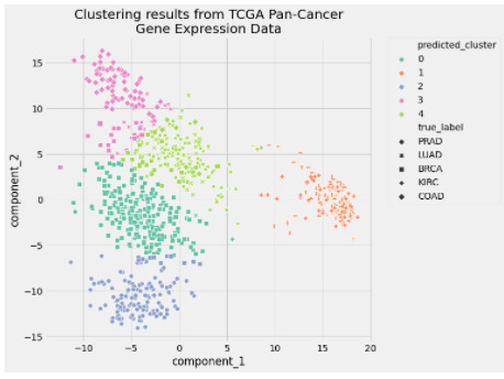
In [4]: data[:5, :3] Out[4]: array([[0.        , 2.01720929, 3.26552691],       [0.        , 0.59273209, 1.58842082],       [0.        , 3.51175898, 4.32719872],       [0.        , 3.66361787, 4.50764878],       [0.        , 2.65574107, 2.82154696]]) In [5]: true_label_names[:5] Out[5]: array(['PRAD', 'LUAD', 'PRAD', 'PRAD', 'BRCA'], dtype='<U4') In [6]: label_encoder = LabelEncoder() In [7]: true_labels = label_encoder.fit_transform(true_label_names) In [8]: true_labels[:5] Out[8]: array([4, 3, 4, 4, 0]) In [9]: label_encoder.classes_ Out[9]: array(['BRCA', 'COAD', 'KIRC', 'LUAD', 'PRAD'], dtype='<U4') In [10]: n_clusters = len(label_encoder.classes_)

In [11]: preprocessor = Pipeline(   ...:     [   ...:         ("scaler", MinMaxScaler()),   ...:         ("pca", PCA(n_components=2, random_state=42)),   ...:     ]   ...: ) In [12]: clusterer = Pipeline(   ...:    [   ...:        (   ...:            "kmeans",   ...:            KMeans(   ...:                n_clusters=n_clusters,   ...:                init="k-means++",   ...:                n_init=50,   ...:                max_iter=500,   ...:                random_state=42,   ...:            ),   ...:        ),   ...:    ]   ...: )

In [13]: pipe = Pipeline(   ...:     [   ...:         ("preprocessor", preprocessor),   ...:         ("clusterer", clusterer)   ...:     ]   ...: ) In [14]: pipe.fit(data) Out[14]: Pipeline(steps=[('preprocessor',                 Pipeline(steps=[('scaler', MinMaxScaler()),                                 ('pca',                                  PCA(n_components=2, random_state=42))])),                ('clusterer',                 Pipeline(steps=[('kmeans',                                  KMeans(max_iter=500, n_clusters=5, n_init=50,                                         random_state=42))]))])

In [15]: preprocessed_data = pipe["preprocessor"].transform(data) In [16]: predicted_labels = pipe["clusterer"]["kmeans"].labels_ In [17]: silhouette_score(preprocessed_data, predicted_labels) Out[17]: 0.5118775528450304 In [18]: adjusted_rand_score(true_labels, predicted_labels) Out[18]: 0.722276752060253 In [19]: pcadf = pd.DataFrame(   ...:     pipe["preprocessor"].transform(data),   ...:     columns=["component_1", "component_2"],   ...: )   ...:   ...: pcadf["predicted_cluster"] = pipe["clusterer"]["kmeans"].labels_   ...: pcadf["true_label"] = label_encoder.inverse_transform(true_labels) In [20]: plt.style.use("fivethirtyeight")   ...: plt.figure(figsize=(8, 8))   ...:   ...: scat = sns.scatterplot(   ...:     "component_1",   ...:     "component_2",   ...:     s=50,   ...:     data=pcadf,   ...:     hue="predicted_cluster",   ...:     style="true_label",   ...:     palette="Set2",   ...: )   ...:   ...: scat.set_title(   ...:     "Clustering results from TCGA Pan-Cancer\nGene Expression Data"   ...: )   ...: plt.legend(bbox_to_anchor=(1.05, 1), loc=2, borderaxespad=0.0)   ...:   ...: plt.show()

[thinzarsaw-blog]

Assignment 4 k-mean cluster

from pandas import Series, DataFrame import pandas as pd import numpy as np import seaborn as sns import matplotlib.pylab as plt from sklearn.model_selection import train_test_split from sklearn import preprocessing from sklearn.metrics import silhouette_score, adjusted_rand_score from sklearn.decomposition import PCA from sklearn.cluster import KMeans from sklearn.pipeline import Pipeline from sklearn.preprocessing import LabelEncoder, MinMaxScaler   #Load the dataset data = pd.read_csv('C:\\Users\\saw\\Documents\\Breast Cancer Wisconsin_Diagnostic.csv') data_clean = data.dropna() data_clean.dtypes data_clean.describe() datafile = "C:\\Users\\saw\\Documents\\Breast Cancer Wisconsin_Diagnostic.csv" labels_file = "C:\\Users\\saw\\Documents\\Breast Cancer Wisconsin_Diagnostic_label.csv" data = np.genfromtxt(     datafile,     delimiter=",",     usecols=range(1, 30),     skip_header=1 ) true_label_names = np.genfromtxt(     labels_file,     delimiter=",",     usecols=(1,),     skip_header=1,     dtype=str ) data[:5, :3] true_label_names[:5] #Encode target label label_encoder = LabelEncoder() true_labels = label_encoder.fit_transform(true_label_names) true_labels[:5] label_encoder.classes_ n_clusters = len(label_encoder.classes_) preprocessor = Pipeline(     [         ("scaler", MinMaxScaler()),         ("pca", PCA(n_components=2, random_state=42)),     ] ) clusterer = Pipeline(    [        (            "kmeans",            KMeans(                n_clusters=n_clusters,                init="k-means++",                n_init=50,                max_iter=500,                random_state=42,            ),        ),    ] ) pipe = Pipeline(     [         ("preprocessor", preprocessor),         ("clusterer", clusterer)     ] ) pipe.fit(data) #Predict the data preprocessed_data = pipe["preprocessor"].transform(data) predicted_labels = pipe["clusterer"]["kmeans"].labels_ silhouette_score(preprocessed_data, predicted_labels) adjusted_rand_score(true_labels, predicted_labels) pcadf = pd.DataFrame(     pipe["preprocessor"].transform(data),     columns=["component_1", "component_2"], ) pcadf["predicted_cluster"] = pipe["clusterer"]["kmeans"].labels_ pcadf["true_label"] = label_encoder.inverse_transform(true_labels) #plot plt.style.use("fivethirtyeight") plt.figure(figsize=(8, 8)) scat = sns.scatterplot(     "component_1",     "component_2",     s=50,     data=pcadf,     hue="predicted_cluster",     style="true_label",     palette="Set2", ) scat.set_title(     "Clustering results from Breast cancer Data" ) plt.legend(bbox_to_anchor=(1.05, 1), loc=2, borderaxespad=0.0)

plt.show()

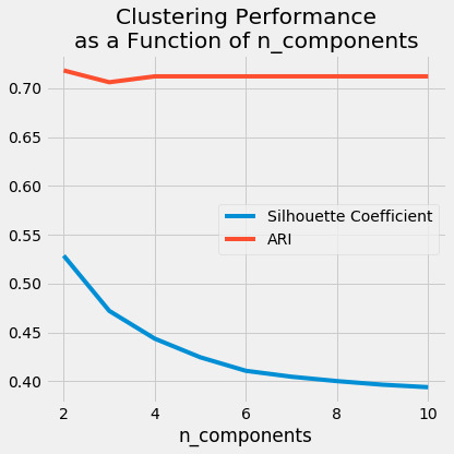
Tuning a K-Means Clustering Pipeline

# Empty lists to hold evaluation metrics silhouette_scores = [] ari_scores = [] for n in range(2, 11):    # This set the number of components for pca,    # but leaves other steps unchanged    pipe["preprocessor"]["pca"].n_components = n    pipe.fit(data)    silhouette_coef = silhouette_score(        pipe["preprocessor"].transform(data),        pipe["clusterer"]["kmeans"].labels_,    )    ari = adjusted_rand_score(        true_labels,        pipe["clusterer"]["kmeans"].labels_,    )    # Add metrics to their lists    silhouette_scores.append(silhouette_coef)    ari_scores.append(ari)

plt.style.use("fivethirtyeight") plt.figure(figsize=(6, 6)) plt.plot(    range(2, 11),    silhouette_scores,    c="#008fd5",    label="Silhouette Coefficient", ) plt.plot(range(2, 11), ari_scores, c="#fc4f30", label="ARI")plt.xlabel("n_components") plt.legend() plt.title("Clustering Performance\nas a Function of n_components") plt.tight_layout() plt.show()

  A k-means cluster analysis was conducted to identify underlying subgroups  based on their similarity of responses on 30 variables that represent characteristics that could have an impact on achievement.  All clustering variables were standardized to have a mean of 0 and a standard deviation of 1.

Data were randomly split into a training set that included 70% of the observations and a test set that included 30% of the observations. A series of k-means cluster analyses were conducted on the training data specifying k=1-9 clusters, using Euclidean distance. The variance in the clustering variables that was accounted for by the clusters (r-square) was plotted for each of the nine cluster solutions in an elbow curve to provide guidance for choosing the number of clusters to interpret.

[livefreeshop]

Abstract: The February 2003 loss of the Space Shuttle Columbia resulted in NASA Management revisiting every critical system onboard this very complex, reusable space vehicle in a an effort to Return to Flight. Many months after the disaster, contact between NASA Johnson Space Center and NASA Glenn Research Center evolved into an in-depth assessment of the actuator drive systems for the Rudder Speed Brake and Body Flap Systems. The actuators are CRIT 1-1 systems that classifies them as failure of any of... from New NASA STI Report Series https://go.nasa.gov/2ompDjk