#spherical polar coordinates

[peeterjoot]

A new version of my book is now published.  The free PDF and the leanpub versions are available now.  The paperback and hardcover versions should be available on Amazon within the week. What has changed: V0.3.2 (Dec 8, 2023) Add to helpful formulas: Determinant form of triple wedge. Add figure showing the spherical polar conventions picked. Add a problem showing that \( (e^x)’ = x’ e^x \) only…

[ltwilliammowett]

Today we're heading into the eternal ice of Antarctica and keeping a special lady company. The beautiful Endurance is waiting for us in door no. 7

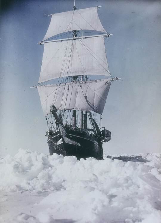
More about her here:

The three-masted schooner barque designed by Ole Aanderud Larsen (1884-1964) was built by the Framnæs shipyard in Sandefjord, Norway. When she was launched on 17 December 1912, she was named Polaris. She was 43.8 m long, 7.62 m wide and weighed 350 tonnes. In addition to square sails on the foremast and gaff sails on the main and mizzen masts, she had a 260 kW steam engine, which allowed a maximum speed of 10 knots (19 km/h). The ship was designed for polar conditions and constructed to minimise the pressure of the ice masses. With a thickness of 28 cm, the frames were made of greenheart wood, a particularly stable type of tropical wood, and were twice as thick as on conventional sailing ships of this size. The hull of the Endurance was designed to be relatively straight-sided, as it was only intended to sail in loose pack ice. She was therefore calmer in the sea than ships with a spherical hull, such as the Fram; however, this came at the cost of not being lifted significantly out of the pressure line in ice pressures and was therefore unsuitable for encasements in pack ice.

The ship was commissioned by the Belgian polar explorer Adrien de Gerlache and the Norwegian whaling magnate Lars Christensen, who actually wanted to use it for polar cruises of a more touristic nature. However, due to financial problems, Christensen was happy to sell his ship to Shackleton for 11,600 pounds sterling (approx. 934,000 euros, as of 2010) - an amount that was less than the original construction costs. Shackleton renamed her Endurance after his family's motto ‘Fortitudine vincimus’ (‘Through endurance we shall conquer’).

The Endurance left the port of Plymouth on 8 August 1914, around a week after Great Britain's entry into the First World War, and completed the journey to Antarctica with a stopover in Buenos Aires without any problems.

Before the crew of the Endurance could cross to the Antarctic mainland to cross the Antarctic as planned, the ship was trapped by the pack ice of the Weddell Sea in January 1915 like ‘an almond in a piece of chocolate’ - as the much-used comparison goes. After resisting the force of the pack ice for 281 days, the Endurance was crushed by the ice on 21 November 1915. The expedition team had previously saved themselves on a safe ice floe. Thanks to a masterly feat of seamanship and navigation, Shackleton and his crew managed to get out of this desolate situation without any losses with the help of three lifeboats that were salvaged from the Endurance.

Initially continuing with the pack ice and later on ice floes, the castaways drifted northwards in their camps along the Antarctic Peninsula until the floes broke into small pieces. They finally reached Elephant Island in their lifeboats. There, one of the boats was converted and set off for South Georgia with 6 men to fetch help, which was successful. Months later, the remaining men who were still stuck on Elephant Island were rescued by a Chilean navy guard boat.

In 2019, a private expedition attempted to locate the wreck of the Endurance, but was unsuccessful.

In January 2022, the Endurance 22 expedition began the search. The S. A. Agulhas II brought the expedition, in which marine physicist Stefanie Arndt from the Alfred Wegener Institute took part,[3] to the last coordinates of the Endurance mentioned. From the historical records, the expedition members knew that the ship must have sunk at ♁68° 39′ 30″ S, 52° 26′ 30″ W. According to the rules of the Antarctic Treaty, the wreck is a protected historical site that may not be touched.

On 5 March 2022, the expedition found the ship with a diving robot at a depth of 3008 m, 7.7 km from the recorded position. Photographs showed the wreck standing upright in excellent condition.

[enetarch-quantum-physics]

Topics to study for Quantum Physics

Calculus

Taylor Series

Sequences of Functions

Transcendental Equations

Differential Equations

Linear Algebra

Separation of Variables

Scalars

Vectors

Matrixes

Operators

Basis

Vector Operators

Inner Products

Identity Matrix

Unitary Matrix

Unitary Operators

Evolution Operator

Transformation

Rotational Matrix

Eigen Values

Coefficients

Linear Combinations

Matrix Elements

Delta Sequences

Vectors

Basics

Derivatives

Cartesian

Polar Coordinates

Cylindrical

Spherical

LaPlacian

Generalized Coordinate Systems

Waves

Components of Equations

Versions of the equation

Amplitudes

Time Dependent

Time Independent

Position Dependent

Complex Waves

Standing Waves

Nodes

AntiNodes

Traveling Waves

Plane Waves

Incident

Transmission

Reflection

Boundary Conditions

Probability

Probability

Probability Densities

Statistical Interpretation

Discrete Variables

Continuous Variables

Normalization

Probability Distribution

Conservation of Probability

Continuum Limit

Classical Mechanics

Position

Momentum

Center of Mass

Reduce Mass

Action Principle

Elastic and Inelastic Collisions

Physical State

Waves vs Particles

Probability Waves

Quantum Physics

Schroedinger Equation

Uncertainty Principle

Complex Conjugates

Continuity Equation

Quantization Rules

Heisenburg's Uncertianty Principle

Schroedinger Equation

TISE

Seperation from Time

Stationary States

Infinite Square Well

Harmonic Oscillator

Free Particle

Kronecker Delta Functions

Delta Function Potentials

Bound States

Finite Square Well

Scattering States

Incident Particles

Reflected Particles

Transmitted Particles

Motion

Quantum States

Group Velocity

Phase Velocity

Probabilities from Inner Products

Born Interpretation

Hilbert Space

Observables

Operators

Hermitian Operators

Determinate States

Degenerate States

Non-Degenerate States

n-Fold Degenerate States

Symetric States

State Function

State of the System

Eigen States

Eigen States of Position

Eigen States of Momentum

Eigen States of Zero Uncertainty

Eigen Energies

Eigen Energy Values

Eigen Energy States

Eigen Functions

Required properties

Eigen Energy States

Quantification

Negative Energy

Eigen Value Equations

Energy Gaps

Band Gaps

Atomic Spectra

Discrete Spectra

Continuous Spectra

Generalized Statistical Interpretation

Atomic Energy States

Sommerfels Model

The correspondence Principle

Wave Packet

Minimum Uncertainty

Energy Time Uncertainty

Bases of Hilbert Space

Fermi Dirac Notation

Changing Bases

Coordinate Systems

Cartesian

Cylindrical

Spherical - radii, azmithal, angle

Angular Equation

Radial Equation

Hydrogen Atom

Radial Wave Equation

Spectrum of Hydrogen

Angular Momentum

Total Angular Momentum

Orbital Angular Momentum

Angular Momentum Cones

Spin

Spin 1/2

Spin Orbital Interaction Energy

Electron in a Magnetic Field

ElectroMagnetic Interactions

Minimal Coupling

Orbital magnetic dipole moments

Two particle systems

Bosons

Fermions

Exchange Forces

Symmetry

Atoms

Helium

Periodic Table

Solids

Free Electron Gas

Band Structure

Transformations

Transformation in Space

Translation Operator

Translational Symmetry

Conservation Laws

Conservation of Probability

Parity

Parity In 1D

Parity In 2D

Parity In 3D

Even Parity

Odd Parity

Parity selection rules

Rotational Symmetry

Rotations about the z-axis

Rotations in 3D

Degeneracy

Selection rules for Scalars

Translations in time

Time Dependent Equations

Time Translation Invariance

Reflection Symmetry

Periodicity

Stern Gerlach experiment

Dynamic Variables

Kets, Bras and Operators

Multiplication

Measurements

Simultaneous measurements

Compatible Observable

Incompatible Observable

Transformation Matrix

Unitary Equivalent Observable

Position and Momentum Measurements

Wave Functions in Position and Momentum Space

Position space wave functions

momentum operator in position basis

Momentum Space wave functions

Wave Packets

Localized Wave Packets

Gaussian Wave Packets

Motion of Wave Packets

Potentials

Zero Potential

Potential Wells

Potentials in 1D

Potentials in 2D

Potentials in 3D

Linear Potential

Rectangular Potentials

Step Potentials

Central Potential

Bound States

UnBound States

Scattering States

Tunneling

Double Well

Square Barrier

Infinite Square Well Potential

Simple Harmonic Oscillator Potential

Binding Potentials

Non Binding Potentials

Forbidden domains

Forbidden regions

Quantum corral

Classically Allowed Regions

Classically Forbidden Regions

Regions

Landau Levels

Quantum Hall Effect

Molecular Binding

Quantum Numbers

Magnetic

Withal

Principle

Transformations

Gauge Transformations

Commutators

Commuting Operators

Non-Commuting Operators

Commutator Relations of Angular Momentum

Pauli Exclusion Principle

Orbitals

Multiplets

Excited States

Ground State

Spherical Bessel equations

Spherical Bessel Functions

Orthonormal

Orthogonal

Orthogonality

Polarized and UnPolarized Beams

Ladder Operators

Raising and Lowering Operators

Spherical harmonics

Isotropic Harmonic Oscillator

Coulomb Potential

Identical particles

Distinguishable particles

Expectation Values

Ehrenfests Theorem

Simple Harmonic Oscillator

Euler Lagrange Equations

Principle of Least Time

Principle of Least Action

Hamilton's Equation

Hamiltonian Equation

Classical Mechanics

Transition States

Selection Rules

Coherent State

Hydrogen Atom

Electron orbital velocity

principal quantum number

Spectroscopic Notation

=====

Common Equations

Energy (E) .. KE + V

Kinetic Energy (KE) .. KE = 1/2 m v^2

Potential Energy (V)

Momentum (p) is mass times velocity

Force equals mass times acceleration (f = m a)

Newtons' Law of Motion

Wave Length (λ) .. λ = h / p

Wave number (k) ..

k = 2 PI / λ

= p / h-bar

Frequency (f) .. f = 1 / period

Period (T) .. T = 1 / frequency

Density (λ) .. mass / volume

Reduced Mass (m) .. m = (m1 m2) / (m1 + m2)

Angular momentum (L)

Waves (w) ..

w = A sin (kx - wt + o)

w = A exp (i (kx - wt) ) + B exp (-i (kx - wt) )

Angular Frequency (w) ..

w = 2 PI f

= E / h-bar

Schroedinger's Equation

-p^2 [d/dx]^2 w (x, t) + V (x) w (x, t) = i h-bar [d/dt] w(x, t)

-p^2 [d/dx]^2 w (x) T (t) + V (x) w (x) T (t) = i h-bar [d/dt] w(x) T (t)

Time Dependent Schroedinger Equation

[ -p^2 [d/dx]^2 w (x) + V (x) w (x) ] / w (x) = i h-bar [d/dt] T (t) / T (t)

E w (x) = -p^2 [d/dx]^2 w (x) + V (x) w (x)

E i h-bar T (t) = [d/dt] T (t)

TISE - Time Independent

H w = E w

H w = -p^2 [d/dx]^2 w (x) + V (x) w (x)

H = -p^2 [d/dx]^2 + V (x)

-p^2 [d/dx]^2 w (x) + V (x) w (x) = E w (x)

Conversions

Energy / wave length ..

E = h f

E [n] = n h f

= (h-bar k[n])^2 / 2m

= (h-bar n PI)^2 / 2m

= sqr (p^2 c^2 + m^2 c^4)

Kinetic Energy (KE)

KE = 1/2 m v^2

= p^2 / 2m

Momentum (p)

p = h / λ

= sqr (2 m K)

= E / c

= h f / c

Angular momentum ..

p = n h / r, n = [1 .. oo] integers

Wave Length ..

λ = h / p

= h r / n (h / 2 PI)

= 2 PI r / n

= h / sqr (2 m K)

Constants

Planks constant (h)

Rydberg's constant (R)

Avogadro's number (Na)

Planks reduced constant (h-bar) .. h-bar = h / 2 PI

Speed of light (c)

electron mass (me)

proton mass (mp)

Boltzmann's constant (K)

Coulomb's constant

Bohr radius

Electron Volts to Jules

Meter Scale

Gravitational Constant is 6.7e-11 m^3 / kg s^2

History of Experiments

Light

Interference

Diffraction

Diffraction Gratings

Black body radiation

Planks formula

Compton Effect

Photo Electric Effect

Heisenberg's Microscope

Rutherford Planetary Model

Bohr Atom

de Broglie Waves

Double slit experiment

Light

Electrons

Casmir Effect

Pair Production

Superposition

Schroedinger's Cat

EPR Paradox

Examples

Tossing a ball into the air

Stability of the Atom

2 Beads on a wire

Plane Pendulum

Wave Like Behavior of Electrons

Constrained movement between two concentric impermeable spheres

Rigid Rod

Rigid Rotator

Spring Oscillator

Balls rolling down Hill

Balls Tossed in Air

Multiple Pullys and Weights

Particle in a Box

Particle in a Circle

Experiments

Particle in a Tube

Particle in a 2D Box

Particle in a 3D Box

Simple Harmonic Oscillator

Scattering Experiments

Diffraction Experiments

Stern Gerlach Experiment

Rayleigh Scattering

Ramsauer Effect

Davisson–Germer experiment

Theorems

Cauchy Schwarz inequality

Fourier Transformation

Inverse Fourier Transformation

Integration by Parts

Terminology

Levi Civita symbol

Laplace Runge Lenz vector

[bad-dagon]

riemann spheres as a fundamental type, pt.1 basics

ive been thinking on and off about riemann spheres for a while now, a couple weeks really, and so far i think there's some utility to them as a building block of a type system of some kind for a joke/toy computer language

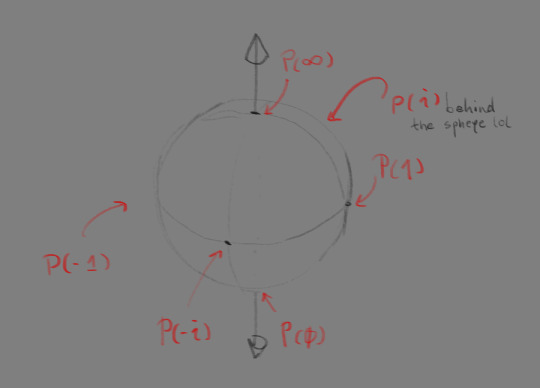
background: riemann spheres are a neat tool in complex analysis where we imagine a sphere whose equator intersects the complex plane, and every number on the complex plane is representable by a point on the sphere such that a line is projected from the north pole and through that point onto the complex plane. naturally, this means that the north pole is P(∞) and the south pole is P(0). see below how that would look like with other unit points of the complex numbers

a neat thing the riemann sphere allows us is to define meaningful division by zero so now z/0 = ∞ clean and simple! and also its inverse, z/∞ = 0 is well behaved as well. this simplifies doing complex analysis but stereographic projection is an absolute bitch to work with turns out, and doing arithmetic on points on the sphere is a mess because it's not a linear mapping (it's continuous though so that's fine)

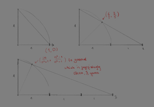
if we're dealing with ONLY real numbers in relation to a circular slice of the riemann sphere, it already starts looking like a mess; for any number n∈R its projective cognate on the circle is located at (2n/n²+1, n²-1/n²+1). on the real riemann sphere though? zoo wee mamma

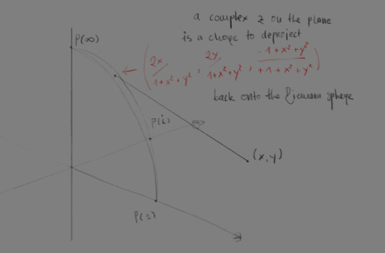
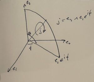
an arbitrary z∈C, represented as a point (x,y) on the complex plane, has to walk through a rather ugly mapping (related to the previous one) to find its point on the sphere; more accurately, given the coordinates (x,y) of the point on the plane, the point on the sphere is located at (2x/1+x²+y², 2y/1+x²+y², -1+x²+y²/1+x²+y²), which is godawful in spherical-to-polar coordinate terms, this is much simpler; for a polar pair (r,θ) the point on the unit sphere representing it is (φ,ξ) = (2*arctg 1/r, θ); and conversely projecting from the riemann sphere is also dead simple, given the zenith-azimuth pair (φ,ξ), (r,θ) = (ctg φ/2, ξ). of course, translating from polar to real coordinates is ALSO dead simple; x = r * cos θ, y = r * sin θ. if a computer system were to store complex numbers (or any coordinate on a 2d plane really), it makes sense to store them in terms of spherical coordinates of a riemann sphere, since this makes infinity well-behaved as a unit (zenith = 0, azimuth = literally who gives a fuck) and is surprisingly efficient. knowing that the zenith is ∈[0,π] and azimuth ∈[0, 2π] can allow for some formidably dumb optimisations that can save on space and ensure granularity. compared to storing them as 2d cartesian or polar coordinates, this provides the benefit of having neither number be larger than like 6.3, so an underlying/backing type that can offer great precision in this small range would be more efficient numerically than, say, floating points which have insane baggage and gaps

or iunno i'll look into that one a bit later, i'm just kind of furious right now that i rederived stereographic projection on my own when the formulas were right fucking there if id only just googled for them

[theohonohan]

Loxodromes, Part 1

Loxodromes (also known as rhumb lines) are a family of curves on the sphere . The family includes meridians (lines of constant longitude) and parallels (lines of constant latitude). The general loxodrome is a spherical spiral which intersects every meridian at the same angle. These curves are useful for navigation, because they describe the idealised course followed by a ship that maintains a constant compass bearing.

The navigator and scientist Thomas Harriot was an early investigator of the loxodrome; he was the first to rectify it (find a mathematical expression for its length) and among the first to rectify any curve. I'm planning to make another post about his method (based on a description in Robin Arianrhod's biography of him). First, though, I'm going to try to give an account of the loxodrome using modern calculus. (I'm leaning on a pretty good treatment on the atractor.pt website.)

The task of deriving the formula for the loxodrome is made much easier by having the right mathematical tools. In this case, the tools are the notion of a parameterised space curve, a vector-valued function, spherical polar coordinates, Cartesian coordinates, and basic differential and integral calculus.

A space curve, parameterised by the variable \(t\), is a function \(\gamma:\,I\rightarrow\mathbb{R}^{3}\), where \(I\subseteq\mathbb{R}\) is an interval, that associates a point \(\gamma\left(t\right)\in\mathbb{R}^{3}\) to each value of a parameter \(t\in I\).

As a first example, consider a meridian as a space curve. We'll use spherical polar coordinates with radius \(r\), longitude \(\theta\) and colatitude \(\varphi\). (Colatitude is latitude \(- \frac{\pi}{2}\): latitude measured from the North Pole.)

The equation of a meridian at longitude \(\theta_p\), as a function of \(\varphi\), is

\[m(\varphi) = (r\cos(\theta_p)\sin(\varphi),r\sin(\theta_p)\sin(\varphi),r\cos(\varphi))\]

The range of \(\varphi\) is \(]0,\pi[\).

Consider a loxodrome \(\ell_\alpha\) that intersects the meridians at angle \(\alpha\).

A fixed point \(P\) on \(\ell_\alpha\) has coordinates \((r, \theta_p, \varphi_p)\).

The fine article on atractor.pt starts with the case of \(\alpha = \frac{\pi}{2} + n+n\pi\), for some \(n\in\mathbb{Z}\). This example covers the loxodromes that coincide with parallels of latitude, and it's a fine warm-up, but not very revealing. Such loxodromes are most straightfordwardly thought of as being parameterized by longitude, \(\theta\).

The general loxodrome, with a spherical spiral form, corresponds to the case \(\alpha \neq \frac{\pi}{2} + n\pi, n\in\mathbb{Z}\).

In this case, the parameterisation of \(\ell_{\alpha}\) is given as a function of colatitude. Because of the nature of the spherical spiral, there is a just one point of the curve at each (co)latitude. Longitude would not work as a parameterisation for a spherical spiral, or at least longitude conventionally limited to the range \(-\pi\) to \(\pi\) would not.

We define a function

\[\begin{array}{ccll} \ell_{\alpha}: & ]0\,,\pi[ & \longrightarrow & \mathbb{S}^{2} \\\\ & \varphi & \mapsto & \left(r\cos\left(\theta_\alpha\left(\varphi\right)\right) \sin\varphi, r\sin\left(\theta_\alpha\left(\varphi\right)\right), r\cos\varphi\right),\end{array}\]

The next step is to find the formulas of the tangents to both the loxodrome \(\ell_\alpha\(\varphi)\) and the meridian \(m(\varphi)\). This is achieved by componentwise differentiation.

\[\begin{array}{rccl}\ell_{\alpha}^{\prime}(\varphi_{P}) & = & & r\,\theta'_\alpha\left(\varphi_{P}\right)\left(-\sin\left(\theta_{P}\right)\sin\left(\varphi_{P}\right)\,,\,\cos\left(\theta_{P}\right)\sin\left(\varphi_{P}\right),0\right)\\\\ & & + & r\left(\cos\left(\varphi_{P}\right)\cos\left(\theta_{P}\right)\,,\,\cos\left(\varphi_{P}\right)\,\sin\left(\theta_{P}\right)\,,\,-\sin\left(\varphi_{P}\right)\right)\end{array}\] and \[m'(\varphi_{P})=r\left(\cos\left(\varphi_{P}\right)\cos\left(\theta_{P}\right)\,,\,\cos\left(\varphi_{P}\right)\,\sin\left(\theta_{P}\right)\,,\,-\sin\left(\varphi_{P}\right)\right)\,.\]

These angle between these two tangents is \(\alpha\). Thus

\[\cos\alpha=\frac{\ell_{\alpha}^{\prime}\left(\varphi_{P}\right)\,|\,m'\left(\varphi_{P}\right)}{\Vert\ell_{\alpha}^{\prime}\left(\varphi_{P}\right)\Vert\times\Vert m'\left(\varphi_{P}\right)\Vert}\,.\]

After some calculating, we get

\[\cos\alpha=\frac{1}{\sqrt{1+[\theta_{\alpha}^{\prime}(\varphi_{P})]^2sin^2(\varphi_{P})}}\]

Isolating \(\theta_{\alpha}^\prime(\varphi_{P})\), we have

\[\theta'_\alpha(\varphi_{P}) = \pm\frac{\tan\alpha}{\sin\left(\varphi_{P}\right)}\]

(This solution is only possible because \(\cos\alpha\) is not \(0\) and \(\varphi\in\ ]0, \pi[\).)

It is now possible to integrate this expression with respect to \(\varphi\) to get a formula for \(\theta_\alpha(\varphi)\): choosing to integrate \(-\frac{\tan\alpha}{\sin\left(\varphi_{P}\right)}\), the formula is \(\theta_\alpha(\varphi)=\tan\alpha\ln\left(\cot\frac{\varphi}{2}\right)+k\), for some constant \(k\in\mathbb{R}\). Since \(\theta_\alpha(\varphi_{P})=\theta_{P}\), we get \(k=\theta_{P}-\tan\alpha\ln\left(\cot\frac{\varphi_{P}}{2}\right)\).

Therefore, if \(\alpha\neq\frac{\pi}{2}+n\pi\), with \(n\in\mathbb{Z}\), then a parametrisation of \(\ell_{\alpha}\) is given by:

\[\begin{array}{ccll}\ell_{\alpha}: & ]0\,,\pi[ & \longrightarrow & \mathbb{S}^{2}\\\\ & \varphi & \mapsto & \left(r\cos\left(\theta_\alpha\left(\varphi\right)\right)\sin\varphi\,,\,r\sin\left(\theta_\alpha\left(\varphi\right)\right)\sin\varphi\,,\, r\cos\varphi\right)\end{array}\,,\] with \(\theta_\alpha(\varphi)=\theta_{P}+\tan\alpha\left[\ln\left(\cot\frac{\varphi}{2}\right)-\ln\left(\cot\frac{\varphi_{P}}{2}\right)\right]\).

This result is less advanced than the formula for the loxodrome that Wikipedia gives. The calculation is "elementary" in the sense that it avoids hyperbolic trig functions and the Gudermannian function (whatever that is). Elementary doesn't mean simple.

[stuart-boehmer]

APROPOS KERR METRIC AND INTERIOR SOLUTION

APROPOS THE VACUUM KERR METRIC AND INTERIOR KERR SOLUTION

Stuart Boehmer

            According to a formula of Tolman (“Relativity, Thermodynamics and Cosmology,” Clarendon Press, 1934), with which apparently most authors are unfamiliar, and which can easily be reproduced with a little careful thought, the relationship between the spatial metric, gmn, and the space-time metric, Gmn, is not gmn = Gmn, but gmn = Gmn – G0mG0n/G00.

            Therefore, a singularity coincident with the ergosphere is found to occur in the g33 component of the spatial metric (where u3 is the longitude), thereby rendering the standard vacuum Kerr metric theoretically useless as a practical model of a rotating black hole (see my prior missive, “Theory of Black Holes,” apropos my thought on singularities occurring in nature—the mathematical trick I used there to render impotent the singularity in g11 at the Schwarzschild radius doesn’t seem to work here).

            Thus, in order to find a practical working model, there seems to be no shortcut except to do the hard work of solving the full, interior problem, including the consequent vacuum solution for the region of space exterior to the rotating dead star. This remains an open problem, but with the assistance of machine computation it is conceptually trivial, as we shall describe presently.

            Define the problem in this way for specificity: use spherical polar coordinates where r is the radial distance from the center along a path of constant co-latitude and longitude (therefore g11 := 1).  I see no reason to complicate matters by using the hyperbolic elliptic coordinate system chosen by Kerr.  The black hole or dead star is assumed to be spherical (density a nonzero constant inside a sphere of radius r = R) and rotating with constant angular velocity w := du3/dt.  Because, as we are about to describe, the solution is in terms of Taylor series, there is no a priori reason we cannot use general functions d(r,u2) and w(r,u2) expanded as Taylor series with known coefficients).

            At this point, allow me to parenthetically describe the process of “Involution” (W. Seiler, Springer, 2009) for solving any differential equation or system of differential equations in terms of Taylor series and justify it as being just as good (and, for purposes of practical calculation in no way inferior to) finding a solution in terms of “elementary” functions—the obsession for which no doubt contributes to the fact that this conceptually trivial problem has remained open so long.  Indeed, this method could be used to solve any problem in any theory of physics and no “open problems” should remain anywhere in the entire discipline of physics, conceptually.

            The method is this: expand all known and unknown functions in terms of Taylor series; the known functions have known coefficients, and the unknown functions have unknown coefficients which can be derived recursively by equating the coefficients of like powers of the coordinates, by the standard procedure.  See what I mean by “trivial?”

            Now some old-fashioned people may object that any sound theory must be construed in terms of “elementary” functions, which are in some sense “known.”  Of course, the only elementary functions except for polynomials are the trigonometric, hyperbolic trigonometric and exponential functions—all of which can be reduced to the exponential function, which in turn can be accurately calculated in terms of—guess what?—Taylor series or some equivalent infinite recursive process.

            These days, we might regard elliptic integrals as elementary functions and there is an elaborate algebraic theory reducing the evaluation of an arbitrary elliptic function to those of the first, second and third kinds, but no one is interested in this theory any longer—it is simpler to just evaluate in terms of Taylor series by machine computation (the “NI” in UNIAC and ENIAC stand for “Numerical Integrator”—that is why computers were invented!).

            Conclusion: computation by machine is just as respectable as any reduction to elementary functions—and there is no escaping the use of machine computation when calculating numerical values of “elementary” functions anyway!

            The method of involution is often described as reducing calculus to algebra, because, of course, machine computation must terminate in a finite number of steps and the Taylor series just turns out to be polynomials of high degree.  Polynomials are, ultimately, the only functions whose numerical values can be computed in a finite number of steps.

[brickwall2]

APROPOS KERR METRIC AND INTERIOR SOLUTION

APROPOS THE VACUUM KERR METRIC AND INTERIOR KERR SOLUTION

Stuart Boehmer

            According to a formula of Tolman (“Relativity, Thermodynamics and Cosmology,” Clarendon Press, 1934), with which apparently most authors are unfamiliar, and which can easily be reproduced with a little careful thought, the relationship between the spatial metric, gmn, and the space-time metric, Gmn, is not gmn = Gmn, but gmn = Gmn – G0mG0n/G00.

            Therefore, a singularity coincident with the ergosphere is found to occur in the g33 component of the spatial metric (where u3 is the longitude), thereby rendering the standard vacuum Kerr metric theoretically useless as a practical model of a rotating black hole (see my prior missive, “Theory of Black Holes,” apropos my thought on singularities occurring in nature—the mathematical trick I used there to render impotent the singularity in g11 at the Schwarzschild radius doesn’t seem to work here).

            Thus, in order to find a practical working model, there seems to be no shortcut except to do the hard work of solving the full, interior problem, including the consequent vacuum solution for the region of space exterior to the rotating dead star. This remains an open problem, but with the assistance of machine computation it is conceptually trivial, as we shall describe presently.

            Define the problem in this way for specificity: use spherical polar coordinates where r is the radial distance from the center along a path of constant co-latitude and longitude (therefore g11 := 1).  I see no reason to complicate matters by using the hyperbolic elliptic coordinate system chosen by Kerr.  The black hole or dead star is assumed to be spherical (density a nonzero constant inside a sphere of radius r = R) and rotating with constant angular velocity w := du3/dt.  Because, as we are about to describe, the solution is in terms of Taylor series, there is no a priori reason we cannot use general functions d(r,u2) and w(r,u2) expanded as Taylor series with known coefficients).

            At this point, allow me to parenthetically describe the process of “Involution” (W. Seiler, Springer, 2009) for solving any differential equation or system of differential equations in terms of Taylor series and justify it as being just as good (and, for purposes of practical calculation in no way inferior to) finding a solution in terms of “elementary” functions—the obsession for which no doubt contributes to the fact that this conceptually trivial problem has remained open so long.  Indeed, this method could be used to solve any problem in any theory of physics and no “open problems” should remain anywhere in the entire discipline of physics, conceptually.

            The method is this: expand all known and unknown functions in terms of Taylor series; the known functions have known coefficients, and the unknown functions have unknown coefficients which can be derived recursively by equating the coefficients of like powers of the coordinates, by the standard procedure.  See what I mean by “trivial?”

            Now some old-fashioned people may object that any sound theory must be construed in terms of “elementary” functions, which are in some sense “known.”  Of course, the only elementary functions except for polynomials are the trigonometric, hyperbolic trigonometric and exponential functions—all of which can be reduced to the exponential function, which in turn can be accurately calculated in terms of—guess what?—Taylor series or some equivalent infinite recursive process.

            These days, we might regard elliptic integrals as elementary functions and there is an elaborate algebraic theory reducing the evaluation of an arbitrary elliptic function to those of the first, second and third kinds, but no one is interested in this theory any longer—it is simpler to just evaluate in terms of Taylor series by machine computation (the “NI” in UNIAC and ENIAC stand for “Numerical Integrator”—that is why computers were invented!).

            Conclusion: computation by machine is just as respectable as any reduction to elementary functions—and there is no escaping the use of machine computation when calculating numerical values of “elementary” functions anyway!

            The method of involution is often described as reducing calculus to algebra, because, of course, machine computation must terminate in a finite number of steps and the Taylor series just turns out to be polynomials of high degree.  Polynomials are, ultimately, the only functions whose numerical values can be computed in a finite number of steps.

[jarviscodinghub]

[SOLUTION] Physics 396 Homework Set 7

1. In spherical-polar coordinates, the line element on the surface of the two-sphere takes the form dS2 = a2 (d✓2 + sin2 ✓d2 ), (1) where a is the constant radius of the sphere. The Christo↵el symbols can be computed from the metric and derivatives of the metric through the expression g↵ = 1 2 ✓@g↵ @x + @g↵ @x @g @x↵ ◆ , (2) where a repeated index implies a sum over that index. For diagonal line…

[codeshive]

Physics 396 Homework Set 7 solved

1. In spherical-polar coordinates, the line element on the surface of the two-sphere takes the form dS2 = a2 (d✓2 + sin2 ✓d2 ), (1) where a is the constant radius of the sphere. The Christo↵el symbols can be computed from the metric and derivatives of the metric through the expression g↵ = 1 2 ✓@g↵ @x + @g↵ @x @g @x↵ ◆ , (2) where a repeated index implies a sum over that index. For diagonal line…

[codingprolab]

Physics 396 Homework Set 7 solved

1. In spherical-polar coordinates, the line element on the surface of the two-sphere takes the form dS2 = a2 (d✓2 + sin2 ✓d2 ), (1) where a is the constant radius of the sphere. The Christo↵el symbols can be computed from the metric and derivatives of the metric through the expression g↵ = 1 2 ✓@g↵ @x + @g↵ @x @g @x↵ ◆ , (2) where a repeated index implies a sum over that index. For diagonal line…

[peeterjoot]

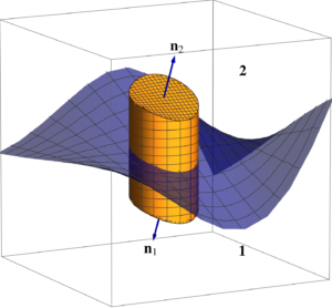
Derivatives of spherical polar vector representation.

[Click here for a PDF version of this post] On discord, on the bivector server, ‘not a good username’ asked a question that I really liked. It’s a question that nagged me before too, but I hadn’t taken the time to puzzle through it properly. The main character in this question is the spherical polar form of a radial vector, which has the…

[10051112x]

WhatsApp +8615146602893howellmed@outlook.comNEUROSURGERY STEREOTACTIC SYSTEM . EASY TO INSTALLON THE OPERATING BED.INDEPENDENT PACKAGING DESIGN, COMPLETEACCESSORIES,EASY TO CARRY. PROFESSIONAL FOCUS ON PROVIDING SKULL SURGERY FRAMECLEAR SCALE LINESALSO EQUIPPED WITH SOFTWARE SYSTEM.The cranial cavity is a limited space. There is a relationship between the position of any structure in the brain and the space of the brain, which can be determined by using the principle of analytic geometric coordinate system. The Cartesian coordinate system is based on the Cartesian principle. Three mutually perpendicular planes are set in the cranial cavity. The x y and z axes of the horizontal, coronal, and sagittal planes intersect at one point. The coordinates of the y and z axes are established; the polar coordinate system is also called the spherical coordinate system, which takes the center of the orientation instrument as the center of the sphere, and any point on the surface of the sphere can be determined by the radius of the sphere and the two angles between the vertical plane and the horizontal plane.

[ferbtv]

even when they talk about the same thing it can be different

genuine warning to anyone taking both physics and math classes:

both mathematicians and physicists use the variables (r, theta, phi) for spherical coordinates. but physicists usually use (r, theta, phi) = (radial, polar, azimuthal) and mathematicians usually use (r, theta, phi) = (radial, azimuthal, polar). the definitions of theta and phi are swapped.

Me in high school: yeah physics and math have a crazy amount of overlap and, you know, in a lot of ways, they talk about the same thing.

Me now, a physics major asking a math major something: I'm sorry what the actual fuck did you just say? What are those words? Why are you speaking like this? Can't you just explain it with numbers?

[thisiswash]

AHA

MY PROFESSOR SAID IT

MY PROFESSOR SAID ROTATION ISNT INTUITIVE

I AM VALIDATED

[undusmundus]

Whoever invented Spherical Coordinates had no reason to go that hard.