akshatkumar01

[akshatkumar01]

Week-4 (Creating graphs)

Variables used :

Explanatory variables - urbanrate, relectricperperson, incomeperperson

Response variable - co2emissions

Since both of my explanatory as well as response variable are quantitative, I have used a scatterplot to examine the association between two variables.

Centre and spread of my variables

d = data['co2emissions'].describe()

print(d)

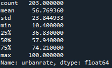
d1 = data['urbanrate'].describe()

print(d1)

d2 = data['relectricperperson'].describe()

print(d2)

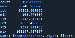
d3 = data['incomeperperson'].describe()

print(d3)

Univariate graph

In the above univariate graph we can see a left skewed distribution.

Basic scatterplot to examine relation between variables

1. Association between urban-rate and CO2 emissions.

scat1 = seaborn.regplot(x = "urbanrate", y = "co2emissions", fit_reg = False, data = data)

plt.xlabel('Urban rate')

plt.ylabel('CO2 emissions')

plt.title('Scatterplot for the association between urbanization rate and co2 emissions.')

The above scatter plot shows that there is strong increasing relationship between urbanization rate and cumulative co2 emissions.

2. Association between residential electric consumption per person and co2 emissions

scat2 = seaborn.regplot(x = "relectricperperson", y = "co2emissions", fit_reg = False, data = data)

plt.xlabel('Electric consumption per person')

plt.ylabel('CO2 emissions')

plt.title('Scatterplot for the association between electric consumption per person and CO2 emission')

In the above plot, we can see a decreasing relation between electric consumption per person and the co2 emissions. So we can say there is an inverse relation between the two variables.

Bivariate graph (categorical to quantitative bar chart)

Firstly using data management, I have converted the numerical values of urbanrate into categorical values.

data['urbanrategrp'] = pandas.qcut(data.urbanrate, 4, labels = ["0-25%", "26-50%", "51-74%", "75-100%"])

u1 = data['urbanrategrp'].value_counts(sort = False, dropna = True)

In the above graph, we can see that it is left skewed and depicts an increasing relation between the Mean CO2 emission and the urbanization rate.

Summary

I can conclude now, that I have successfully examined the association between co2 emissions and urbanization rate. I have found out that countries having a lower urban rate have lower co2 emissions when compared to countries with a higher urban rate.

[akshatkumar01]

Data Management

1. Program

import pandas

import numpy

#bug fix for display formats to avoid runtime errors

pandas.set_option('display.float_format', lambda x : '%f' %x)

data = pandas.read_csv('gapminder.csv', low_memory = False)

sub1 = data[(data["country"] == "India" )]

sub2 = sub1.copy()

d = sub2["polityscore"] = sub2["polityscore"].replace(9, numpy.nan)

sub2["polityscore"] = sub2["polityscore"] + sub2["urbanrate"]

2. Output

3. Summary

Here, we consider the variables for the country "India". This helps in localizing the problem and I can study the relation between co2emissions and urbanrate in India.

[akshatkumar01]

First Program

1. Program

import pandas

import numpy

pandas.set_option('display.float_format', lambda x : '%f' %x)

data = pandas.read_csv('gapminder.csv', low_memory = False)

print(len(data))

print(len(data.columns))

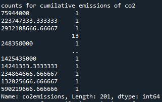
print("counts for cumilative emissions of co2")

c1 = data['co2emissions'].value_counts(sort = False, dropna = False)

print(c1)

print("percentage for cumilative emissions of co2")

p1 = data['co2emissions'].value_counts(sort = False, normalize = True)

print(p1)

print("counts for urbanrate")

c2 = data['urbanrate'].value_counts(sort = False, dropna = False)

print(c2)

print("percentage for urbanrate")

p2 = data['urbanrate'].value_counts(sort = False, normalize = True)

print(p2)

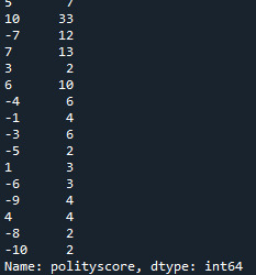
print("counts for polityscore")

c3 = data['polityscore'].value_counts(sort = False, dropna = False)

print(c3)

print("percentage for polityscore")

p3 = data['polityscore'].value_counts(sort = False, normalize = True)

print(p3)

2. Output:

213 (number of rows in the data set)

16 (number of columns in the data set)

3. Summary

I have taken frequency distributions for three variables from the gapminder data set. Missing data is also considered by using "dropna".

The first distribution is of the co2emissions. It is a quantitative variable and it takes integer values which indicate co2 emissions of each country in metric tonnes.

The second distribution is of the urbanrate. It indicates what proportion of a country's population is urbanized. It takes integer values of how many countries have a particular urbanization rate.

The third distribution is of the polityscore. It is a measure of a country's democratic and free measure. It takes integer values ranging from -10 to 10, where -10 indicates lowest polity score and 10 the highest. It is also listed in the output how many countries have a specific polity score.

[akshatkumar01]

PROJECT

After going through the gapminder codebook, I have decided that I am interested in carbon dioxide emissions globally and how they are correlated with the rate of increase in urbanization in various countries. Therefore, I have selected the gapminder data set.

Research question: Are the cumulative CO2 emissions globally affected by the urban ratio of various countries?

Hypotheses:

1. Urbanization has lead to an increase in consumption of fossil fuels such as oil, natural gas etc. consequently increasing the emissions of CO2.

2. Economic growth in developing countries demands for a higher consumption of energy subsequently increasing electricity generation.

3. Countries having a higher GDP per capita tends to an increase in CO2 emissions.

For this I intend to use variables of: CO2emissions, urbanrate, incomeperperson, polityscore, oilperperson, relectricperperson.

Literature review:

Cycling of carbon (C) is essential to processes that provide food, fiber, and fuel for all of the Earth's inhabitants. On one hand, carbon dioxide is the second most abundant greenhouse gas after water vapor in the Earth's atmosphere. Together with other greenhouse gases it keeps our planet warm, with a danger to overheat if the concentrations of the greenhouse gases become too high. On the other hand, photosynthetic organisms such as plants and algae take up atmospheric CO2 in the presence of light to produce organic matter that eventually becomes the basic food source for all microbes, animals, and humans. Carbon-based molecules are the main component of biological compounds as well as of many minerals. Carbon containing compounds also exist in various forms in the atmosphere. Availability of all these different forms of carbon makes our planet suitable for humans to survive.

Although our planet offers a vast amount of space, humans prefer to live in cities, which occupy a small area of the total land surface (~0.5% Schneider et al., 2009). Given the tendency to consider it a local phenomenon, urbanization has been excluded from global studies of the carbon cycle. Yet urbanization trends and emerging evidence of urban pressure on the environment present persuasive arguments for reconsidering this view. The share of the urban population has already increased by 40% over one century (1913–2013) and will increase by another 15% in the next 50 years (FAO, 2015). Land area occupied by cites increases disproportionally faster to the population increase (Seto et al., 2011). Population pressure on the environment is especially high in the tropics. Urban expansion in the tropics contributes ~5% of global emissions from deforestation and land use change (Seto et al., 2012). In addition to that it is widely known that approximately 75% of global CO2 emissions originate in urban areas (Seto et al., 2014). Carbon storage in human settlements of the conterminous US was ~10% of the total carbon stored in the US ecosystems (Churkina et al., 2010a). In China, this fraction was substantially smaller—only 0.74% and this did not include C stored in landfills (Zhao et al., 2013). Although carbon budget assessments are in progress for several cities (e.g., Mohareb and Kennedy, 2012; Hutyra et al., 2014), the overall effect of urbanization on the global carbon cycle has not been estimated.

The IPCC (2014) reveals that CO2 emission from industrial processes and fossil fuel combustion shared 78% increase in overall Greenhouse gas emission from 1970 to 2010. The CO2 emission since seventies has more than doubled and increased by 40% since 2000. Despite of having stability during 2013 to 2016, the CO2 emission have increased by 1.5% in 2017 and continue to increase led by China, India and EU [7]. The lack of policy measures, the emission trends are expected to increase profoundly due to increased global energy demand and fossil fuels being the main drivers of greenhouse gas emissions which will ultimately have negative effects on public health.

Countries in Far East Asia such as Japan, China, South Korea, Malaysia, Singapore, Thailand and Hong Kong have achieved rapid economic growth in last few decades due to division of labor and development of non-agricultural sectors has resulted into an increased urbanization. These countries are among the largest economies of the world with majority of their population lives in urban areas (i.e., 91%, 57.96%, 81.50%, 75.44%, 100%, 49.2% and 100% respectively). These economies with high level of growth and urbanization have contributed enormously to CO2 emissions in recent times. Japan, China and South Korea were responsible for 12 percent of the total CO2 emissions in 1980 and 18 percent in 2013. Despite having high level of economic growth, urbanization and CO2 emission, limited cross country studies have examined the association among urbanization, economic growth and CO2 emission in these Far East Asian countries.

References:

The Role of Urbanization in the Global Carbon Cycle : https://doi.org/10.3389/fevo.2015.00144

Impact of Urbanization and Economic Growth on CO2 Emission: A Case of Far East Asian Countries: https://www.researchgate.net/publication/340510260_Impact_of_Urbanization_and_Economic_Growth_on_CO2_Emission_A_Case_of_Far_East_Asian_Countries