allthingsverification

[allthingsverification]

Metadata register checks

Metadata means usually anything (something like residue) that we need to check post packet transmission or reception

[allthingsverification]

Difference between Dynamic Array and Assosicate Array in SystemVerilog

With a regular array, you must specify its size when you declare it bit my_array[10]; With a dynamic array you can allocate the size of the array during runtime (hence the term "dynamic"). bit my_dynamic_array[];  // Note size is not specified ... my_dynamic_array = new[size];  // size is determined at run-time Also, the array can be "re-sized" at a later point: my_dynamic_array = new[new_size](my_dynamic_array); In this case, new memory is allocated, and the old array values are copied into the new memory, giving the effect of resizing the array. The main characteristic of an associative array is that the index type can be any type - you are not restricted to just integer values. For example, you can use a string as the index to look up an "associated" value. bit my_assoc_array[string];  // Array stores bits, using a string as an index ... my_assoc_array["testname"] = 1;  //Stores a 1 into the array element indexed by the value "testname" $display(my_assoc_array["testname"]); // Displays 1 An associative array is also "dynamic", in the sense that it does not have a pre-determined size. However, you do not have to allocate the size - it grows as you add more elements into it. Another answer is:    Dynamic arrays are useful for dealing with contiguous collections of variables whose number changes dynamically.    e.g.            int array[];    When the size of the collection is unknown or the data space is sparse (scattered-throw in various random directions.), an associative array is a better option. In associative array, it uses the transaction names as the keys in associative array.   e.g.            int array[string];

[allthingsverification]

Pass by ref and pass by value #SV

Difference between pass by ref and pass by value?

Pass by value is the default method through which arguments are passed into functions and tasks. Each subroutine retains a local copy of the argument. If the arguments are changed within the subroutine declaration, the changes do not affect the caller. In pass by reference functions and tasks directly access the specified variables passed as arguments.Its like passing pointer of the variable. In verilog,method arguments takes as pass by value.The inputs are copyed when the method is called and the outputs are assigned to outputs when exiting the method.In SystemVerilog ,methods can have pass by reference.Arguments passed by reference are not copied into the subroutine area, rather, a reference to the original argument is passed to the subroutine. The subroutine can then access the argument data via the reference. In the following example, variable a is changed at time 10,20 and 30. The method pass_by_val , copies only the value of the variable a, so the changes in variable a which are occurred after the task pass_by_val call, are not visible to pass_by_val. Method pass_by_ref is directly referring to the variable a. So the changes in variable a are visible inside pass_by_ref. EXAMPLE: program main();  int a;  initial begin    #10 a = 10;    #10 a = 20;    #10 a = 30;    #10 $finish;  end  task pass_by_val(int i);    forever      @i $display("pass_by_val: I is %0d",i);  endtask  task pass_by_ref(ref int i);    forever begin      @i $display("pass_by_ref: I is %0d",i);    end  endtask  initial begin    pass_by_val(a);  end  initial begin    pass_by_ref(a);  end endprogram RESULT: pass_by_ref: I is 10 pass_by_ref: I is 20 pass_by_ref: I is 30 By default, SystemVerilog passes arrays by value, copying the entire array. It is recommended to pass arrays by reference whenever possible for performance reasons. If you want your function to modify the array, use ref. If you want your function to read the array, use const ref. Example: module automatic test;  initial run();  function void run();    // Create some SystemVerilog arrays and populate them    int array[5];    int queue[$];    int assoc[int];    for (int i = 0; i < 5; i++) begin      array[i] = i;      queue[i] = i;      assoc[i] = i;    end        pass_by_value(array, queue, assoc);    $display("After pass by value:");    for (int i = 0; i < 5; i++) begin      $display("array[%0d]:%0d", i, array[i]);      $display("queue[%0d]:%0d", i, queue[i]);      $display("assoc[%0d]:%0d", i, assoc[i]);    end      pass_by_ref(array, queue, assoc);    $display("After pass by reference:");    for (int i = 0; i < 5; i++) begin      $display("array[%0d]:%0d", i, array[i]);      $display("queue[%0d]:%0d", i, queue[i]);      $display("assoc[%0d]:%0d", i, assoc[i]);    end      endfunction   // These functions try to modify the arrays.   // Default.   // A copy of the arrays is made in this function   function void pass_by_value(int array[5], int queue[$], int assoc[int]);    array[2] = 100;    queue[2] = 100;    assoc[2] = 100;  endfunction   // Original arrays are being referenced   function void pass_by_ref(ref int array[5], ref int queue[$], ref int assoc[int]);    array[3] = 100;    queue[3] = 100;    assoc[3] = 100;    endfunction     // Original arrays are being referenced   // And they can be read but cannot be modified in this function   function void pass_by_const_ref(const ref int array[5],                                  const ref int queue[$],                                  const ref int assoc[int]);    // Arrays cannot be modified in this function    // array[3] = 100;    // queue[3] = 100;    // assoc[3] = 100;    endfunction endmodule

[allthingsverification]

UVM command line

The growing complexity of ASIC/FPGA designs in recent era has caused simulation times to increase drastically. This is because there is a growing need to ensure that the simulation matches the expectations of a business outcome-driven verification environment. In any case, the compilation of complex designs and test bench remains the single biggest concern for any verification engineer. The more flexibility you have in your VE to simulate design again and again without compiling the bulky complex design, the more time you can save which can be used in other important tasks during design verification phase. Such flexibility includes simulating designs with Test bench reconfigurations, applying effective constraints to important control knobs (like altering the lower or upper cap of control variables) etc.

The ability to change the configuration or parameters without being forced to recompile can result in significant time savings. UVM (Universal Verification Methodology) is the most powerful methodology that has become the most cutting-edge and popular SV methodology in the verification world. At eInfochips, we have been successfully leveraging complex projects in networking, consumer devices, automotive, smartphones, camera equipment, multimedia, aerospace, servers, automated test equipment, and MEMS. As per one of our clients, have perfected the art, so as to speak.

As such, there are many things recommended for a user to follow in various UVM manuals but in this article, we will discuss one of the most powerful – no, THE most powerful feature of UVM which is “uvm_cmdline_processor”. Effective usage of “uvm_cmdline_processor” can lead to remarkable time savings in any design verification project.

What is UVM COMMANDLINE PROCESSOR?

The class of “uvm_cmdline_processor” provides a general interface to command line arguments that were provided for any given simulation. The “uvm_cmdline_processor” class also provides support for setting up various UVM variables from the command line such as components’ verbosities and configuration settings for integral types and strings. With a same compiled database, it allows more flexible and useful controls to run tests with different values of many control variables and ultimately, it can help cover more scenarios with less number of tests.

“uvm_cmdline_processor” has various in-built methods like get_args(), get_plusargs(), get_uvm_args() and get_arg_matches() to retrieve command line arguments. The “get_arg_values” can be used to retrieve the suffix values of an argument. Based on any given scenario needed, the required constraints can be applied to other variables of a test. Let’s talk of one of the methods “get_arg_value()” in more detail to understand possible usage with few examples.

get_arg_value (arg, value)

This function is used to get the value of specific command line argument(s). For a VE having multiple possible configurations, the “get_arg_value” function can be used to run the same test with all different configurations, without re-compiling test bench again and again. That too without changing test(s) or sequence(s).

Example 1:

VE with PCIe as an interface protocol, taking into account the operating speed and number of lanes for which there are multiple configurations possible. VE can have multiple APIs targeted to configure specific speeds and number of lanes. Based on command line arguments like +link_speed and +lanes, a same set of test sequences can be run with all possible configurations. If user wants to run a test with PCIe speed = Gen2 and lanes = x2, then this can be achieved simply by having +link_speed=gen2 and +lanes=2 on command line arguments, and in verification environment fetching them by calling methods like get_arg_value(“+link_speed=”,link_speed) and get_arg_value(“+lanes=”, lanes) while using local variables (link_speed and lanes) in respective APIs.

Example 2:

User can control address range randomization through command line arguments. Such a control would really help in functional coverage closure where a set of tests can be run with desired control value(s) to hit functional coverage holes. Example codes in below snippet shows how one can control the generation of addresses using this method.

Figure 1: CLA to control address randomization

Example 3:

To verify the HDMI transmitter and receiver, there are many possible test cases based on proposed framework. Instead of developing many tests, multiple scenarios can be generates if the height and width information is controlled from the command line. If user wants to run a test with width=640 and height=480, then on the command line, all he needs to do is pass +width=640 and +height=480. The verification environment fetches these values by calling methods as get_arg_value(“+width=”,width) and get_arg_value(“+height=”, height).

So, as explained in above examples, any desired VE field can be controlled from command line itself to simulate more scenarios using same set of tests/sequences.

In addition, the “uvm_cmdline_processor” class has in-built UVM aware commands for better simulation control. Following are a few use cases.

Changing test configuration

For a complex design where compilation as well as simulation consumes lots of time (lengthy simulations), one can change any variable to desired value without recompile using UVM-aware commands like “+uvm_set_config_int=” and “+uvm_set_config_string=”.

As shown in below snippet, if the need is to override a variable “scb_en” in an environment class, then it is achieved by adding command line option as,

+uvm_set_config_int=uvm_test_top.env,scb_en,1

Figure 2: Overriding configuration control variable

Using above method, ”scb_en” variable is set to value 1 that overrides the initial value.

Additional Built-in UVM Aware Command Line Arguments

+UVM_TESTNAME

It allows the user to specify which uvm_test should be created via the factory and run through the UVM phases. Desired selected tests can be run using this option without recompiling test bench and design.

Example:

+UVM_TESTNAME=write_read_rst_read_test

+UVM_TESTNAME=fifo_ovfl_err_test

+UVM_VERBOSITY

It allows the user to specify initial verbosity for all UVM components. By default, it is set to UVM_MEDIUM OR UVM_LOW based on the EDA tool in use.

Example:

+UVM_VERBOSITY=UVM_HIGH

+UVM_VERBOSITY=UVM_LOW

Using “+uvm_set_verbosity“, the user can also change the verbosity of specific component at specific phases of the simulation.

Example:

+uvm_set_verbosity=uvm_test_top.env.agent_A.*,_ALL_,UVM_FULL,time,800

+UVM_TIMEOUT:

It allows the user to change the global timeout of the UVM framework.

Syntax is +UVM_TIMEOUT=<timeout>,<overridable>

The <overridable> argument (‘YES’ or ‘NO’) specifies whether user code can subsequently change this value

Example:

+UVM_TIMEOUT=2000000,NO

Changing Max Quit Count

Using in built +UVM_MAX_QUIT_COUNT command line option, user can change the max quit count for the report server to any desired value.

Example:

By adding “+UVM_MAX_QUIT_COUNT=5” in command line the test simulation ends when it encounters total 5 errors.

Summary:

To summarize, the effective usage of in-built methods of “uvm_cmdline_processor” can result in huge time savings to meet the verification deadlines and for timely completion of a verification project. Same set of test cases and sequences can be reused to make more meaningful scenarios by controlling various configurations and control knobs using in-built methods of uvm_cmdline_processor.

eInfochips has been working with hundreds of clients on V&V projects, of which UVM methodology has been a real value addition.

[allthingsverification]

https://blog.verificationgentleman.com/2014/03/10/a-subtle-gotcha-when-using-forkjoin.html

A Subtle Gotcha When Using fork…join

March 10, 2014

I want to start things out light with a recent experience I've had using fork...join statements.

My intention was to start several parallel threads inside a for loop and have them take the loop parameter as an input. I naively assumed the following code would do the job:

module top;  initial begin    for (int i = 0; i < 3; i++)      fork        some_task(i);      join_none  end  task some_task(int i);    $display("i = %d", i);  endtask endmodule

Do you see the problem with this code? If not, don't worry as I didn't at first either. Here is the output if you run it:

# i =           3 # i =           3 # i =           3

It seems that the for loop executed completely and only then did the spawned processes start, but they were given the latest value of i.

After digging around on the Internet I discovered the answer. The SystemVerilog LRM mentions that "spawned processes do not start executing until the parent thread executes a blocking statement". This explains why the for loop finished executing and why by the time the processes were spawned i had already reached the value '3'.

The LRM also shows exactly how to fix our problem: "Automatic variables declared in the scope of the fork...join block shall be initialized to the initialization value whenever execution enters their scope, and before any processes are spawned". Applying this to our code yields:

module top;  initial begin    for (int i = 0; i < 3; i++)      fork        automatic int j = i;        some_task(j);      join_none  end  task some_task(int i);    $display("i = %d", i);  endtask endmodule

Now, for every loop iteration a new variable is allocated, which is then passed to the respective task. Running this example does indeed give the desired result:

# i =           2 # i =           1 # i =           0

I've been playing with parallel processes for quite some time now, but I didn't know about this until recently. I've mostly learned SystemVerilog from online tutorials, but I see that a quick read of the LRM might be of real use. Who knows what other tricks are in there?

I'll keep you updated with any more subtleties I find.

[allthingsverification]

Important to remember

1K (KILO) = 2^10

1M (MEGA) = 2^20

1G (GIGA) = 2^30 

1T (TERRA) = 2^40 

[allthingsverification]

Interface SV

An interface is a named bundle of wires, the interfaces aim is to encapsulate communication. 

It also specifies: Directional information i.e modports, timing information i.e clocking blocks

An interface can have parameters, constants, variables, functions and tasks. 

[allthingsverification]

Performance Basics

Utilization: The percentage of time that a device is busy servicing requests

Utilization = (Device Busy Time/Total Time) * 100

The remaining percentage of time is idle time

Idle Time = 100 - Utilization 

Throughput: The amount of work completed by the system per unit of time 

There is an upper bound on how much work a system can complete per unit of time. 

Observed bandwidth is one measure of throughput

ex: MB/sec, ops/sec, tpmc, WIPs, frames/sec 

Choose an appropriate throughput metric

Path length & CPI(Cycles per instruction) determines throughput

-> Lower pathlength( with same or lower CPI) - Better throughput

-> Lower CPI with same or lower pathlength - Better throughput

Note: In Industry we use IPC (Instructions per cycle) instead of CPI. IPC should be high for better throughput 

Latency/Response Time

Loosely speaking: 

Latency is the time interval between when any request for data is made and when the data transfer completes. 

Latency is also referred to as Response Time

Technically speaking:

Latency = Request to first data 

Response time = Request to transfer complete

Response time = Latency + Transfer time

Response time can be viewed as a cumulative sum of several response time of subtasks. {Except they sometimes overlap}

There is a queuing relationship between response time and throughput. Optimizing for one may hurt the other. 

Concurrency: 

Number of work items that can be completed simultaneously (threads, executables etc)

Concurrency can be used to reduce effective latency and/or increase observed total throughput

Some problems parallelism friendly: If 1 painter takes 10 hrs, 10 painters take 1 hr. 

Some aren’t: If 1 boat crosses ocean in 10 days, 10 boats cross in 10 days 

But you get 10 boats every 10 days. If you pipeline, you can get 1 boat per day. Bandwidth increase, no latency drop. 

Some need new algorithms 

Bottlenecks: 

Bottlenecks are the slowest parts of a system. Often called hotspots. 

Points of serialization exist when work must wait for other work to be finished. 

The bottleneck eventually determines how much work a system can do per unit time. 

The primary bottleneck determines the maximum throughput in a system 

Removing one bottleneck may expose another. 

Multi-Processing

The ability to execute multiple processes or programs on a single system 

On systems with multiple processors, multi-processing may improve throughput. 

- Remember, processors aren’t the only resource. 

-The processor may not be a bottleneck 

Multi-Threading 

The number of execution paths in a program that can execute simultaneously 

Systems that support multi-threading can improve individual application performance by overlapping a high latency request from one thread with low latency requests from another thread for e.g. doing computations for thread 2 while thread 1 is waiting for a memory request. 

Useful for improving latency of a single task 

Scalability

The ability to increase performance by increasing numbers of resources, for example adding CPUs 

Commonly used with SMP systems to indicate the ability to take advantage of the multiple CPUs { SMP is symmetric multiple processing} 

Many possible measures of scalability

- On a fixed workload, the relative improvement in performance with increasing CPUs

- With a scalable workload, the ability to maintain performance with increasing workload and CPUs 

Core Scaling: Performance scaling as we add more cores to each socket

Frequency Scaling: Performance scaling as processors get faster

Cache Scaling: Performance scaling with cache size

Memory Scaling: Performance scaling with memory size

System Scaling: Performance scaling in balanced system 

Not all applications benefit with more resources

[allthingsverification]

AMBA Basics

[allthingsverification]

Clocking Block

A clocking block specifies timing and synchronization for a group of signals. 

The clocking block specifies:

1. The clock event that provides a synchronization reference for DUT and testbench

2. The set of signals that will be sampled and driven by the testbench

3. The timing, relative to the clock event, that the testbench uses to drive and sample those signals

Clocking block can be declared in interface, module or program block. 

clocking cb @(posedge clk);

  default input #1 output #2;

  input from_Dut;

  outut to_Dut;

endclocking

Clocking block terminologies

Clocking event

The event specification used to synchronize the clocking block, @(posedge clk) is the clocking event.

Clocking signal

Signals sampled and driven by the clocking block, from_DUT and to_DUT are the clocking signals,

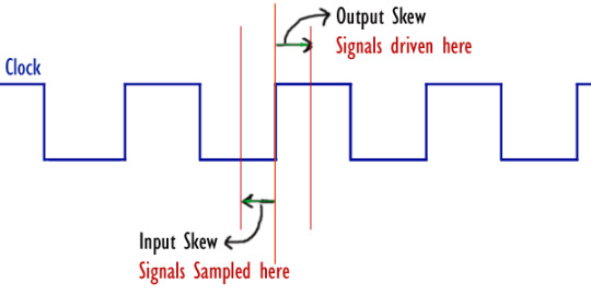
Clocking skew

Clocking skew specifies the moment (w.r.t clock edge) at which input and output clocking signals are to be sampled or driven respectively. A skew must be a constant expression and can be specified as a parameter.

In the above example, the delay values #1 and #2 are clocking skews.

Input and Output skews

Input (or inout) signals are sampled at the designated clock event. If an input skew is specified then the signal is sampled at skew time units before the clock event. Similarly, output (or inout) signals are driven skew simulation time units after the corresponding clock event.

A skew must be a constant expression and can be specified as a parameter. In case if the skew does not specify a time unit, the current time unit is used.

clocking cb @(posedge clk);

 default input #1ps output #2;

 input from_Dut;

 output to_Dut;

endclocking

clocking cb @(clk);

 input #4ps from_Dut;

 output #6 to_Dut;

endclocking

Clocking Block events: 

The clocking event of a clocking block is available directly by using the clocking block name, regardless of the actual clocking event used to declare the clocking block. 

For instance for clocking block cb we can have :

@(cb); 

Which would mean @(clk) {Look last definition of cb} 

Cycle Delay : ##

## operator can be used to delay execution by a specified number of cloking events, or clock cycles. 

Example: ##8;  // Wait 8 clock cycles

## (a +1); // Wait a+1 clock cycles 

[allthingsverification]

System Verilog Mailbox Example

In the example,

Mailbox is used for communication between generator and driver. 

Process 1 (Generator class) will generate (created and randomize) the packet and put it into the mailbox 

Process 2 (Driver class) gets the generated packer from the mailbox and display the fields

/////////// Packet ////////////////

class packet;

   rand bit[7:0] addr;

   rand bit[7:0] data;

 function void post_randomize();

     $display(”Packet::Packet Generated”);

     $display(”Packet::Addr=%0d, Data=%0d”, addr, data);

  endfunction

endclass

///////////Generator - Generates the transaction packet and send to driver//////

class generator;

  packet pkt;

  mailbox m_box;

function new(mailbox m_box);

   this.m_box = m_box; 

endfunction

task run;

   repeat(2) begin

     pkt = new();

     pkt.randomize();

     m_box.put(pkt);

     $display(”Generator:: Packet put into Mailbox”);

    #5;

   end

endtask

endclass

/////////Driver - Gets the packet from generator and display’s the packet items///////

class driver;

  packet pkt;

   mail_box m_box;

    function new(mail_box m_box);

     this.m_box = m_box;

     endfunction

task run;

  repeat(2) begin

   m_box.get(pkt);

   $display(”Driver::Packet Received”);

   $display(”Driver::Addr=%0d, Data=%0d\n”, pkt.addr, pkt.data);

   end

endtask

endclass

/////////////////Test bench Top//////////////////////////////////

module mailbox_ex;

  generator gen;

  driver dri;

  mailbox m_box;

initial begin

m_box = new();

gen =new(m_box);

dri = new(m_box);

$display(”---------------------------------------”);

fork 

  gen.run();

  dri.run();

join

$display(”--------------------------------------”);

end

endmodule

Output : 

------------------------------------------ Packet::Packet Generated Packet::Addr=3,Data=38 Generator::Packet Put into Mailbox Driver::Packet Recived Driver::Addr=3,Data=38 Packet::Packet Generated Packet::Addr=118,Data=92 Generator::Packet Put into Mailbox Driver::Packet Recived Driver::Addr=118,Data=92 ------------------------------------------

[allthingsverification]

Mailbox

A mailbox is a communication mechanism that allows messages to be exchanged between processes. The process which wants to talk to another process posts the message to a mailbox, which stores the messages temporarily in a system defined memory object, to pass it to the desired process.

Based on the sizes mailboxes are categorized as,

bounded mailbox

unbounded mailbox

A bounded mailbox is with the size defined. mailbox becomes full when on storing a bounded number of messages. A process that attempts to place a message into a full mailbox shall be suspended until enough space becomes available in the mailbox queue.

Unbounded mailboxes are with unlimited size.

Mailbox types

There are two types of mailboxes,

Generic Mailbox

Parameterized mailbox

Generic Mailbox (type-less mailbox)

The default mailbox is type-less. that is, a single mailbox can send and receive data of any type.

mailbox mailbox_name;

Parameterized mailbox (mailbox with particular type)

Parameterized mailbox is used to transfer a data of particular type.

mailbox#(type) mailbox_name;

Mailbox Methods

SystemVerilog Mailbox is a built-in class that provides the following methods. these are applicable for both Generic and Parameterized mailboxes

new();Createa mailbox

put(); Place a message in a mailbox

try_put(); Try to place a message in a mailbox without blocking

get(); or peek(); Retrieve a message from a mailbox

num(); Returns the number of messages in the mailbox

try_get(); or try_peek(); Try to retrieve a message from a mailbox without blocking

new( ); 

Mailboxes are created with the new() method.

mailbox_name=new(); // Creates unbounded mailbox and returns mailbox handle

mailbox_name=new(m_size); //Creates bounded mailbox with size m_size and returns mailbox handle ,where m_size is integer  variable

[allthingsverification]

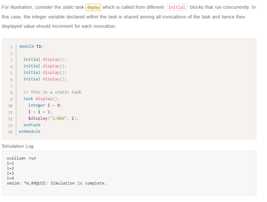
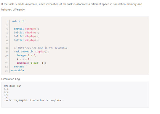
Automatic Task

sniThe keyword automatic will make the task reentrant, otherwise it will be static by default. All items inside automatic tasks are allocated dynamically for each invocation and not shared between invocations of the same task running concurrently. 

Note: Automatic task items cannot be accessed by hierarchical references. 

[allthingsverification]

Semaphores

Semaphore is a SystemVerilog built-in class, used for access control to shared resources, and for basic synchronization.

A semaphore is like a bucket with the number of keys. Processes using semaphores must first procure a key from the bucket before they can continue to execute, All other processes must wait until a sufficient number of keys are returned to the bucket.

Imagine a situation where two processes try to access a shared memory area. where one process tries to write and the other process is trying to read the same memory location. This leads to an unexpected result. A semaphore can be used to overcome this situation.

Semaphore syntax

semaphore semaphore_name;

Semaphore methods

Semaphore is a built-in class that provides the following methods,

new(); Create a semaphore with a specified number of keys

get();   Obtain one or more keys from the bucket

put();   Return one or more keys into the bucket

try_get(); Try to obtain one or more keys without blocking

new( );

The new() method is used to create the Semaphore.

semaphore_name = new(numbers_of_keys);

the new method will create the semaphore with number_of_keys keys in a bucket; where number_of_keys is integer variable.

the default number of keys is ‘0’

the new() method will return the semaphore handle or null if the semaphore cannot be created

put( );

The semaphore put() method is used to return key/keys to a semaphore.

semaphore_name.put(number_of_keys);

or

semaphore_name.put();

When the semaphore_name.put() method is called, the specified number of keys are returned to the semaphore. The default number of keys returned is 1.

get( );

The semaphore get() method is used to get key/keys from a semaphore.

semaphore_name.get(number_of_keys);

or

semaphore_name.get();

When the semaphore_name.get() method is called,

If the specified number of keys are available, then the method returns and execution continues

If the specified number of keys are not available, then the process blocks until the keys become available

The default number of keys requested is 1

try_get();

The semaphore try_get() method is used to procure a specified number of keys from a semaphore, but without blocking.

semaphore_name.try_get(number_of_keys);

or

semaphore_name.try_get();

When the semaphore_name.try_get() method is called,

If the specified number of keys are available, the method returns 1 and execution continues

If the specified number of keys are not available, the method returns 0 and execution continues

The default number of keys requested is 1

Semaphore examples

two processes accessing the same resource

In the example below, semaphore sema is created with the 1 key, two processes are accessing the display method at the same time, but only one process will get the semaphore key and the other process will wait till it gets the key.

module semaphore_ex;

semahore sema;

initial begin 

  sema = new(1);

 fork 

  display();

  display();

 join

end

task automatic display();

   sema.get();

  $display($time,”\t Current Simulation Time”);

  #30;

  sema.put();

endtask 

endmodule

Simulator Output: 

0 Current Simulation Time

30 Current Simulation Time

[allthingsverification]

Interesting scenario

https://stackoverflow.com/questions/19792938/how-can-i-use-foreach-and-fork-together-to-do-something-in-parallel

[allthingsverification]

RAM Vrs CAM

Difference between Random Access Memory (RAM) and Content Addressable Memory (CAM)

Last Updated : 13 May, 2019

RAM: Random Access Memory (RAM) is used to read and write. It is the part of primary memory and used in order to store running applications (programs) and program’s data for performing operation. It is mainly of two types: Dynamic RAM (or DRAM) and Static RAM (or SRAM).

CAM: Content Addressable Memory (CAM) is also known as Associative Memory, in which the user supplies data word and associative memory searches its entire memory and if the data word is found, It returns the list of addresses where that data word was located.

The difference table is given below on the basis of their properties:

S.NORAM MemoryAssociative Memory(CAM)

{1st line for RAM, 2nd for CAM}

1.RAM stands for Random Access Memory.

1. It stands for Content Addressable Memory.

2.In RAM, the user supplies a memory address and RAM returns data word stored at the address.

2. In associative memory, the user supplies data word and associative memory searches its entire memory.

3.The price of RAM is low as compared to Associative memory.

3. It is expensive than RAM.

4.It is used to store running applications(programs) and program’s data for performing operation.

4. It is widely used in database management system.

5.This is suitable for algorithm based search via PRAM. 

5. PRAM stands for Parallel-RAM.This is suitable for parallel search.

6.If the data word is found, RAM returns the data word.

6. If the data word is found, It returns the list of addresses where that data word was located.

[allthingsverification]

Associative Arrays

ASSOCIATIVE ARRAYS Dynamic arrays are useful for dealing with contiguous collections of variables whose number changes dynamically. Associative arrays give you another way to store information. When the size of the collection is unknown or the data space is sparse, an associative array is a better option. In Associative arrays Elements Not Allocated until Used. Index Can Be of Any Packed Type, String or Class. Associative elements are stored in an order that ensures fastest access. In an associative array a key is associated with a value. If you wanted to store the information of various transactions in an array, a numerically indexed array would not be the best choice. Instead, we could use the transaction names as the keys in associative array, and the value would be their respective information. Using associative arrays, you can call the array element you need using a string rather than a number, which is often easier to remember. The syntax to declare an associative array is: data_type array_id [ key _type]; data_type is the data type of the array elements. array_id is the name of the array being declared. key_type is the data-type to be used as an key. Examples of associative array declarations are: int array_name[*];//Wildcard index. can be indexed by any integral datatype. int array_name [ string ];// String index int array_name [ some_Class ];// Class index int array_name [ integer ];// Integer index typedef bit signed [4:1] Nibble; int array_name [ Nibble ]; // Signed packed array Elements in associative array elements can be accessed like those of one dimensional arrays. Associative array literals use the '{index:value} syntax with an optional default index. //associative array of 4-state integers indexed by strings, default is '1. integer tab [string] = '{"Peter":20, "Paul":22, "Mary":23, default:-1 }; Associative Array Methods SystemVerilog provides several methods which allow analyzing and manipulating associative arrays. They are: The num() or size() method returns the number of entries in the associative array. The delete() method removes the entry at the specified index. The exists() function checks whether an element exists at the specified index within the given array. The first() method assigns to the given index variable the value of the first (smallest) index in the associative array. It returns 0 if the array is empty; otherwise, it returns 1. The last() method assigns to the given index variable the value of the last (largest) index in the associative array. It returns 0 if the array is empty; otherwise, it returns 1. The next() method finds the entry whose index is greater than the given index. If there is a next entry, the index variable is assigned the index of the next entry, and the function returns 1. Otherwise, the index is unchanged, and the function returns 0. The prev() function finds the entry whose index is smaller than the given index. If there is a previous entry, the index variable is assigned the index of the previous entry, and the function returns 1. Otherwise, the index is unchanged, and the function returns 0. EXAMPLE module assoc_arr; int temp,imem[*]; initial begin imem[ 2'd3 ] = 1; imem[ 16'hffff ] = 2; imem[ 4'b1000 ] = 3; $display( "%0d entries", imem.num ); if(imem.exists( 4'b1000) ) $display("imem.exists( 4b'1000) "); imem.delete(4'b1000); if(imem.exists( 4'b1000) ) $display(" imem.exists( 4b'1000) "); else $display(" ( 4b'1000) not existing"); if(imem.first(temp)) $display(" First entry is at index %0db ",temp); if(imem.next(temp)) $display(" Next entry is at index %0h after the index 3",temp); // To print all the elements alone with its indexs if (imem.first(temp) ) do $display( "%d : %d", temp, imem[temp] ); while ( imem.next(temp) ); end endmodule RESULT 3 entries imem.exists( 4b'1000) ( 4b'1000) not existing First entry is at index 3b Next entry is at index ffff after the index 3 3 : 1 65535 : 2