anuja05

[anuja05]

A k-means cluster analysis was conducted to identify underlying subgroups of houses based on their similarity of features on 18 variables that represent characteristics of the houses that could have an impact on the grades provided to the house. Clustering variables included price of the house, bedrooms, bathrooms, measurement of the house in square foot, measurement of the lot in square foot, floors, whether a house has a view to waterfront, whether a house has been viewed or not, condition of a house on a scale of 1 to 5, overall grade given to the housing unit based on grading system on a scale of 1 to 11, square footage of house apart from basement, square footage of the basement of the house, years since house is built, years since house is renovated, zip code, latitude, longitude, living room area in 2015, lot size area in 2015. All clustering variables were standardized to have a mean of zero and a standard deviation of one. Data were randomly split into a training set that included 70% of the observations (N= 1145) and a test set that included 30% of the observations (N= 491).  A series of k-means cluster analyses were conducted on the training data specifying k=1-9 clusters, using Euclidean distance. The average distance from observations was plotted for each of the nine cluster solutions in an elbow curve to provide guidance for choosing the number of clusters to interpret.  

Elbow curve From the below figure, 3 or 4 cluster solutions might be interpreted.

Canonical discriminant analyses was used to reduce the 18 clustering variable down a few variables that accounted for most of the variance in the clustering variables. A scatterplot of the first two canonical variables by cluster (Figure 2 shown below) indicated that the observations in 2 and 3 clusters are densely packed with relatively low within cluster variance and did not overlap very much with the other clusters. Cluster 1 observations had greater spread suggesting higher within cluster variance.

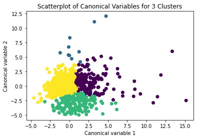
Here the size of cluster 4 is too small also is has higher within cluster variation.

 The results of above both plots suggest that the best cluster solution will be 3 clusters.

The means on the clustering variables showed that, compared to the other clusters, houses in cluster 1 had moderate levels on the clustering variables. They had moderate house prices with moderate numbers of bedrooms. The size of the living house is also moderate compared to other clusters. Houses in cluster 2 have low prices compared to other clusters. Even their number of bedrooms and bathrooms, area under living house is low. Exception is the number of years since the house was built is moderate. Cluster 3 can be classified as the expensive and high graded houses as they have the highest price compared to other 2 clusters. Their number of bedrooms and bathrooms, also the living area and the area under the lot is highest. They have highest number of floors along with maximum area in the basement.

In order to externally validate the clusters, an Analysis of Variance (ANOVA) was conducting to test for significant differences between the clusters on grade assigned to these houses. A tukey test was used for post hoc comparisons between the clusters. Results indicated significant differences between the clusters on Grades (p<.0001). The tukey post hoc comparisons showed significant differences between clusters on Grades, with the exception that clusters 1 and 2 were not significantly different from each other. Adolescents in cluster 3 had the highest Grades (mean=1.98, sd=0.83), and cluster 2 had the lowest Grades (mean=1.21, sd=0.44).

Codes-

from pandas import Series, DataFrame

import pandas as pd

import numpy as np

import matplotlib.pylab as plt

from sklearn.cross_validation import train_test_split

from sklearn import preprocessing

from sklearn.cluster import KMeans

"""

Data Management

"""

data = pd.read_csv('kc_house_data.csv')

#upper-case all DataFrame column names

data.columns = map(str.upper, data.columns)

# subset clustering variables

cluster=data[['PRICE','BEDROOMS','BATHROOMS','SQFT_LIVING','SQFT_LOT','FLOORS','WATERFRONT',

'VIEW','CONDITION','SQFT_ABOVE','SQFT_BASEMENT','YR_BUILT','YR_RENOVATED','ZIPCODE',

'LAT','LONG','SQFT_LIVING15','SQFT_LOT15']]

cluster.describe()

# standardize clustering variables to have mean=0 and sd=1

clustervar=cluster.copy()

from sklearn import preprocessing

clustervar['PRICE']=preprocessing.scale(clustervar['PRICE'].astype('float64'))

clustervar['BEDROOMS']=preprocessing.scale(clustervar['BEDROOMS'].astype('float64'))

clustervar['BATHROOMS']=preprocessing.scale(clustervar['BATHROOMS'].astype('float64'))

clustervar['SQFT_LIVING']=preprocessing.scale(clustervar['SQFT_LIVING'].astype('float64'))

clustervar['SQFT_LOT']=preprocessing.scale(clustervar['SQFT_LOT'].astype('float64'))

clustervar['FLOORS']=preprocessing.scale(clustervar['FLOORS'].astype('float64'))

clustervar['WATERFRONT']=preprocessing.scale(clustervar['WATERFRONT'].astype('float64'))

clustervar['VIEW']=preprocessing.scale(clustervar['VIEW'].astype('float64'))

clustervar['CONDITION']=preprocessing.scale(clustervar['CONDITION'].astype('float64'))

clustervar['SQFT_ABOVE']=preprocessing.scale(clustervar['SQFT_ABOVE'].astype('float64'))

clustervar['SQFT_BASEMENT']=preprocessing.scale(clustervar['SQFT_BASEMENT'].astype('float64'))

clustervar['YR_BUILT']=preprocessing.scale(clustervar['YR_BUILT'].astype('float64'))

clustervar['YR_RENOVATED']=preprocessing.scale(clustervar['YR_RENOVATED'].astype('float64'))

clustervar['ZIPCODE']=preprocessing.scale(clustervar['ZIPCODE'].astype('float64'))

clustervar['LAT']=preprocessing.scale(clustervar['LAT'].astype('float64'))

clustervar['LONG']=preprocessing.scale(clustervar['LONG'].astype('float64'))

clustervar['SQFT_LIVING15']=preprocessing.scale(clustervar['SQFT_LIVING15'].astype('float64'))

clustervar['SQFT_LOT15']=preprocessing.scale(clustervar['SQFT_LOT15'].astype('float64'))

# split data into train and test sets

clus_train, clus_test = train_test_split(clustervar, test_size=.3, random_state=123)

# k-means cluster analysis for 1-9 clusters                                                           

from scipy.spatial.distance import cdist

clusters=range(1,10)

meandist=[]

for k in clusters:

    model=KMeans(n_clusters=k)

    model.fit(clus_train)

    clusassign=model.predict(clus_train)

    meandist.append(sum(np.min(cdist(clus_train, model.cluster_centers_, 'euclidean'), axis=1))

    / clus_train.shape[0])

"""

Plot average distance from observations from the cluster centroid

to use the Elbow Method to identify number of clusters to choose

"""

plt.plot(clusters, meandist)

plt.xlabel('Number of clusters')

plt.ylabel('Average distance')

plt.title('Selecting k with the Elbow Method')

# Interpret 3 cluster solution

model3=KMeans(n_clusters=3)

model3.fit(clus_train)

clusassign=model3.predict(clus_train)

# plot clusters

from sklearn.decomposition import PCA

pca_2 = PCA(2)

plot_columns = pca_2.fit_transform(clus_train)

plt.scatter(x=plot_columns[:,0], y=plot_columns[:,1], c=model3.labels_,)

plt.xlabel('Canonical variable 1')

plt.ylabel('Canonical variable 2')

plt.title('Scatterplot of Canonical Variables for 3 Clusters')

plt.show()

"""

BEGIN multiple steps to merge cluster assignment with clustering variables to examine

cluster variable means by cluster

"""

# create a unique identifier variable from the index for the

# cluster training data to merge with the cluster assignment variable

clus_train.reset_index(level=0, inplace=True)

# create a list that has the new index variable

cluslist=list(clus_train['index'])

# create a list of cluster assignments

labels=list(model3.labels_)

# combine index variable list with cluster assignment list into a dictionary

newlist=dict(zip(cluslist, labels))

newlist

# convert newlist dictionary to a dataframe

newclus=DataFrame.from_dict(newlist, orient='index')

newclus

# rename the cluster assignment column

newclus.columns = ['cluster']

# now do the same for the cluster assignment variable

# create a unique identifier variable from the index for the

# cluster assignment dataframe

# to merge with cluster training data

newclus.reset_index(level=0, inplace=True)

# merge the cluster assignment dataframe with the cluster training variable dataframe

# by the index variable

merged_train=pd.merge(clus_train, newclus, on='index')

merged_train.head(n=100)

# cluster frequencies

merged_train.cluster.value_counts()

"""

END multiple steps to merge cluster assignment with clustering variables to examine

cluster variable means by cluster

"""

# FINALLY calculate clustering variable means by cluster

clustergrp = merged_train.groupby('cluster').mean()

print ("Clustering variable means by cluster")

print(clustergrp)

# validate clusters in training data by examining cluster differences in GRADE using ANOVA

# first have to merge GRADE with clustering variables and cluster assignment data

GRADE_data=data['GRADE']

# split GPA data into train and test sets

GRADE_train, GRADE_test = train_test_split(GRADE_data, test_size=.3, random_state=123)

GRADE_train1=pd.DataFrame(GRADE_train)

GRADE_train1.reset_index(level=0, inplace=True)

merged_train_all=pd.merge(GRADE_train1, merged_train, on='index')

sub1 = merged_train_all[['GRADE', 'cluster']].dropna()

import statsmodels.formula.api as smf

import statsmodels.stats.multicomp as multi

GRADEmod = smf.ols(formula='GRADE ~ C(cluster)', data=sub1).fit()

print (GRADEmod.summary())

print ('means for GRADE by cluster')

m1= sub1.groupby('cluster').mean()

print (m1)

print ('standard deviations for GRADE by cluster')

m2= sub1.groupby('cluster').std()

print (m2)

mc1 = multi.MultiComparison(sub1['GRADE'], sub1['cluster'])

res1 = mc1.tukeyhsd()

print(res1.summary())

print ('standard deviations for GPA by cluster')

m2= sub1.groupby('cluster').std()

print (m2)

mc1 = multi.MultiComparison(sub1['GPA1'], sub1['cluster'])

res1 = mc1.tukeyhsd()

print(res1.summary())

[anuja05]

Lasso Regression for predicting sales price of house

To perform lasso regression the housing data was considered where the response variable is the price of the house and 18 explanatory variables were used. The explanatory variables used were bedrooms, bathrooms, measurement of the house in square foot, , measurement of the lot in square foot, floors, whether a house has a view to waterfront, whether a house has been viewed or not, condition of a house on a scale of 1 to 5, overall grade given to the housing unit based on grading system on a scale of 1 to 11, square footage of house apart from basement, square footage of the basement of the house, years since house is built, years since house is renovated, zip code, latitude, longitude, living room area in 2015, lot size area in 2015. All predictor variables were standardized to have a mean of zero and a standard deviation of one.

Data were randomly split into a training set that included 70% of the observations (N=15129) and a test set that included 30% of the observations (N=6484). The least angle regression algorithm with k=5 fold cross validation was used to estimate the lasso regression model in the training set, and the model was validated using the test set. The change in the cross validation average (mean) squared error at each step was used to identify the best subset of predictor variables.

Below chart specifies the change in mean square error at each step

Of the 18 explanatory variables 17 were retained in the model. Area of the living house in square foot and overall grade given to the house were strongly associated with the response variable price of the house followed by years since the house is built and waterfront view. Years required to built the house is negatively associated with response variable while the other 3 are positively associated. This 17 explanatory variables explained 71% of the variability in predicting the price of the house.

Codes - ##Importing Libraries import pandas as pd import numpy as np import matplotlib.pylab as plt from sklearn.model_selection import train_test_split from sklearn.linear_model import LassoLarsCV #Reading the data data = pd.read_csv('kc_house_data.csv') #upper-case all DataFrame column names data.columns = map(str.upper, data.columns) data.describe() data.info() data.isnull().sum() #select predictor variables and target variable as separate data sets

predvar= data[['BEDROOMS','BATHROOMS','SQFT_LIVING','SQFT_LOT','FLOORS','WATERFRONT', 'VIEW','CONDITION','GRADE','SQFT_ABOVE','SQFT_BASEMENT','YR_BUILT','YR_RENOVATED','ZIPCODE', 'LAT','LONG','SQFT_LIVING15','SQFT_LOT15']] target = data.PRICE #scaling the explanatory variables

predictors=predvar.copy() from sklearn import preprocessing predictors['BEDROOMS']=preprocessing.scale(predictors['BEDROOMS'].astype('float64')) predictors['BATHROOMS']=preprocessing.scale(predictors['BATHROOMS'].astype('float64')) predictors['SQFT_LIVING']=preprocessing.scale(predictors['SQFT_LIVING'].astype('float64')) predictors['SQFT_LOT']=preprocessing.scale(predictors['SQFT_LOT'].astype('float64')) predictors['FLOORS']=preprocessing.scale(predictors['FLOORS'].astype('float64')) predictors['WATERFRONT']=preprocessing.scale(predictors['WATERFRONT'].astype('float64')) predictors['VIEW']=preprocessing.scale(predictors['VIEW'].astype('float64')) predictors['CONDITION']=preprocessing.scale(predictors['CONDITION'].astype('float64')) predictors['GRADE']=preprocessing.scale(predictors['GRADE'].astype('float64')) predictors['SQFT_ABOVE']=preprocessing.scale(predictors['SQFT_ABOVE'].astype('float64')) predictors['SQFT_BASEMENT']=preprocessing.scale(predictors['SQFT_BASEMENT'].astype('float64')) predictors['YR_BUILT']=preprocessing.scale(predictors['YR_BUILT'].astype('float64')) predictors['YR_RENOVATED']=preprocessing.scale(predictors['YR_RENOVATED'].astype('float64')) predictors['ZIPCODE']=preprocessing.scale(predictors['ZIPCODE'].astype('float64')) predictors['LAT']=preprocessing.scale(predictors['LAT'].astype('float64')) predictors['LONG']=preprocessing.scale(predictors['LONG'].astype('float64')) predictors['SQFT_LIVING15']=preprocessing.scale(predictors['SQFT_LIVING15'].astype('float64')) predictors['SQFT_LOT15']=preprocessing.scale(predictors['SQFT_LOT15'].astype('float64')) #split data into train and test sets pred_train, pred_test, tar_train, tar_test = train_test_split(predictors, target, test_size=.3, random_state=123) pred_train.shape, pred_test.shape, tar_train.shape, tar_test.shape #specify the lasso regression model model=LassoLarsCV(cv=5, precompute=False).fit(pred_train,tar_train) #print variable names and regression coefficients dict(zip(predictors.columns, model.coef_)) #plot coefficient progression m_log_alphas = -np.log10(model.alphas_) ax = plt.gca() plt.plot(m_log_alphas, model.coef_path_.T) plt.axvline(-np.log10(model.alpha_), linestyle='--', color='k', label='alpha CV') plt.ylabel('Regression Coefficients') plt.xlabel('-log(alpha)') plt.title('Regression Coefficients Progression for Lasso Paths') #plot mean square error for each fold m_log_alphascv = -np.log10(model.cv_alphas_) plt.figure() plt.plot(m_log_alphascv, model.mse_path_, ':') plt.plot(m_log_alphascv, model.mse_path_.mean(axis=-1), 'k', label='Average across the folds', linewidth=2) plt.axvline(-np.log10(model.alpha_), linestyle='--', color='k', label='alpha CV') plt.legend() plt.xlabel('-log(alpha)') plt.ylabel('Mean squared error') plt.title('Mean squared error on each fold') #MSE from training and test data from sklearn.metrics import mean_squared_error train_error = mean_squared_error(tar_train, model.predict(pred_train)) test_error = mean_squared_error(tar_test, model.predict(pred_test)) print ('training data MSE') print(train_error) print ('test data MSE') print(test_error) #R-square from training and test data rsquared_train=model.score(pred_train,tar_train) rsquared_test=model.score(pred_test,tar_test) print ('training data R-square') print(rsquared_train) print ('test data R-square') print(rsquared_test)

[anuja05]

Random Forest model to predict attrition

Random forest analysis was performed to evaluate the importance of a series of explanatory variables in predicting a binary, categorical response variable. For analysis the aim was to predict attrition of employees and uncover the factors that lead to employee attrition.

The following explanatory variables were included in Random forest model evaluating attrition(my response variable) – Age, Business Travel(Rarely, Frequently, Non travel), Daily rate, Department, Distance from home, education, education field, environment satisfaction (Low, medium, high), gender, hourly rate, Job involvement, job level, Job Role, Job Satisfaction, Marital Status, Monthly Income, Monthly Rate, Number of Companies Worked, Over Time, Percent Salary Hike, Performance Rating, Relationship Satisfaction, Stock Option Level, Total Working Years, Training Times Last Year, Work Life Balance, Years At Company, Years In Current Role, Years Since Last Promotion, Years With Current Manager.

The data size considered was 1470 and the categorical variables were transformed into dummies. The data was split into train (60) and test (40) and the model was built on train dataset.

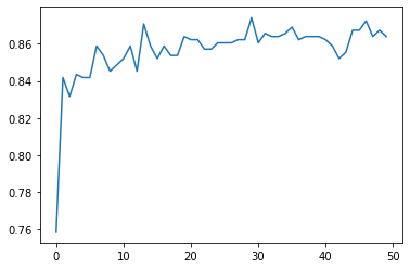
The explanatory variables with the highest relative importance scores were Monthly rate, Overtime, Daily rate, Age, Hourly Rate and total working years. The variable with lowest importance was Performance rating. The accuracy of the random forest was 86%, with the subsequent growing of multiple trees rather than a single tree, adding little to the overall accuracy of the model, and suggesting that interpretation of a single decision tree may be appropriate.

In the below image the x axis represents the number of trees while the y axis represents the accuracy of the model. Here we can observe with a single decision tree the accuracy of the model will be around 84% but as the number of trees increases the accuracy increases to 86%.

Codes - #importing libraries from sklearn.model_selection import train_test_split import pandas as pd from sklearn.ensemble import RandomForestClassifier import sklearn.metrics #Reading the data df = pd.read_csv('HR_EmployeeAttrition.csv')

df.describe() df.info() df.isnull().sum() df.dtypes

#dropping columns df.drop(['EmployeeCount', 'EmployeeNumber', 'Over18', 'StandardHours'], axis="columns", inplace=True)

#Converting ,categorical columns to dummies categorical_col = [] for column in df.columns: if df[column].dtype == object and len(df[column].unique()) <= 50: categorical_col.append(column)

df['Attrition'] = df.Attrition.astype("category").cat.codes categorical_col.remove('Attrition') 

from sklearn.preprocessing import LabelEncoder label = LabelEncoder() for column in categorical_col: df[column] = label.fit_transform(df[column]) #Separating response and explanatory variables y = df['Attrition'] X = df.drop(['Attrition'],axis = 1) #Creating train and test data pred_train, pred_test, tar_train, tar_test = train_test_split(X, y, test_size = 0.4, random_state = 0) pred_train.shape, pred_test.shape, tar_train.shape, tar_test.shape #Random forest model rf_clf = RandomForestClassifier(n_estimators=50) rf_clf.fit(pred_train,tar_train)

#Predict the response for test dataset predictions_rf = rf_clf.predict(pred_test)

#confusion matrix sklearn.metrics.confusion_matrix(tar_test,predictions) Output -array([[494, 1], [ 79, 14]], dtype=int64)

#accuracy sklearn.metrics.accuracy_score(tar_test,predictions) Output - 0.8639455782312925 print(rf_clf.feature_importances_)

import numpy as np trees=range(50) accuracy=np.zeros(50)

for idx in range(len(trees)): classifier=RandomForestClassifier(n_estimators=idx+1) classifier=classifier.fit(pred_train,tar_train) predictions = classifier.predict(pred_test) accuracy[idx]=sklearn.metrics.accuracy_score(tar_test,predictions) plt.cla plt.plot(trees,accuracy)

[anuja05]

Decision tree model for employee attrition

Decision tree analysis was performed to test nonlinear relationships among a series of explanatory variables and a binary, categorical response variable. For analysis the aim was to predict attrition of employees and uncover the factors that lead to employee attrition.

The following explanatory variables were included in classification tree model evaluating attrition(my response variable) – Age, Business Travel(Rarely, Frequently, Non travel), Daily rate, Department, Distance from home, education, education field, environment satisfaction (Low, medium, high), gender, hourly rate, Job involvement, job level, Job Role, Job Satisfaction, Marital Status, Monthly Income, Monthly Rate, Number of Companies Worked, Over Time, Percent Salary Hike, Performance Rating, Relationship Satisfaction, Stock Option Level, Total Working Years, Training Times Last Year, Work Life Balance, Years At Company, Years In Current Role, Years Since Last Promotion, Years With Current Manager.

The data size considered was 1470 and the categorical variables were transformed into dummies. The data was split into train (60) and test (40) and the model was built on train dataset.

The Monthly Income was the first variable to separate the sample into two subgroups. If the monthly income of the employee is less than 2437.5 then the observations move to the left side of the split which is 123 out of 882 observations. From this node further split is made on variable Overtime. Similarly, if the monthly income is greater than 2437. 5 then observations move to the right side which includes 759 of the 882 training sample observations. Even this node is splitted further on the variable Overtime. Further splits in the tree can be observed in the diagram. The accuracy of the model was 79%.

Codes - #importing libraries from sklearn.model_selection import train_test_split import pandas as pd from sklearn.tree import DecisionTreeClassifier import sklearn.metrics #Reading the data df = pd.read_csv('HR_EmployeeAttrition.csv')

df.describe() df.info() df.isnull().sum() df.dtypes

#dropping columns df.drop(['EmployeeCount', 'EmployeeNumber', 'Over18', 'StandardHours'], axis="columns", inplace=True)

#Converting ,categorical columns to dummies categorical_col = [] for column in df.columns: if df[column].dtype == object and len(df[column].unique()) <= 50: categorical_col.append(column)

df['Attrition'] = df.Attrition.astype("category").cat.codes categorical_col.remove('Attrition')

from sklearn.preprocessing import LabelEncoder label = LabelEncoder() for column in categorical_col: df[column] = label.fit_transform(df[column]) #Separating response and explanatory variables y = df['Attrition'] X = df.drop(['Attrition'],axis = 1) #Creating train and test data pred_train, pred_test, tar_train, tar_test = train_test_split(X, y, test_size = 0.4, random_state = 0) pred_train.shape, pred_test.shape, tar_train.shape, tar_test.shape #Create Decision Tree classifer object clf = DecisionTreeClassifier()

#Train Decision Tree Classifer clf = clf.fit(pred_train,tar_train)

#Predict the response for test dataset predictions = clf.predict(pred_test) #confusion matrix sklearn.metrics.confusion_matrix(tar_test,predictions) Output - array([[428, 67], [ 63, 30]], dtype=int64)

#accuracy sklearn.metrics.accuracy_score(tar_test,predictions) Output - 0.7789115646258503 #Display the tree from IPython.display import Image from six import StringIO from sklearn.tree import export_graphviz import pydot

features = list(df.columns) features.remove("Attrition") dot_data = StringIO() export_graphviz(clf, out_file=dot_data, feature_names=features, filled=True) graph = pydot.graph_from_dot_data(dot_data.getvalue()) Image(graph[0].create_png())