awesomesriram-blog1

[awesomesriram-blog1]

Assignment_4 Testing a Potential Moderator

Chi-Square Test of Independence

#“libraries”

import pandas import numpy import scipy.stats import seaborn import matplotlib.pyplot as plt

data = pandas.read_csv(‘addhealth_pds.csv’, low_memory=False)

#print ('Converting variables to numeric’)

data['H1SU1’] = pandas.to_numeric(data['H1SU1’], errors='coerce’) data['H1NB6’] = pandas.to_numeric(data['H1NB6’], errors='coerce’)

#print ('Coding missing values’)

data[“H1SU1”] = data[“H1SU1”].replace(6, numpy.nan) data[“H1SU1”] = data[“H1SU1”].replace(9, numpy.nan) data[“H1SU1”] = data[“H1SU1”].replace(8, numpy.nan) data[“H1NB6”] = data[“H1NB6”].replace(6, numpy.nan) data[“H1NB6”] = data[“H1NB6”].replace(8, numpy.nan)

#print ('contingency table of observed counts’)

ct1=pandas.crosstab(data['H1SU1’], data['H1NB6’]) print (ct1)

print ('column percentages’) colsum=ct1.sum(axis=0) colpct=ct1/colsum print(colpct)

#print ('chi-square value, p value, expected counts’) cs1= scipy.stats.chi2_contingency(ct1) print (cs1)

#print ('set variable types’) data[“H1NB6”] = data[“H1NB6”].astype('category’) data['H1SU1’] = pandas.to_numeric(data['H1SU1’], errors='coerce’)

seaborn.factorplot(x=“H1NB6”, y=“H1SU1”, data=data, kind=“bar”, ci=None) plt.xlabel('Happiness Level Living in Neighbourhood 5=Very Happy’) plt.ylabel('Considered Suicide in Past 12 Months’)

recode1= {1: 1, 2: 2} data['COMP1v2’]= data[“H1NB6”].map(recode1)

#print ('contigency table of observed counts’) ct2=pandas.crosstab(data['H1SU1’], data['COMP1v2’]) print (ct2)

#print ('column percentages’) colsum=ct2.sum(axis=0) colpct=ct2/colsum print(colpct)

#print ('chi-square value, p value, expected counts’) cs2= scipy.stats.chi2_contingency(ct2) print (cs2)

recode2= {1: 1, 3: 3} data['COMP1v3’]= data[“H1NB6”].map(recode2)

#print ('contigency table of observed counts’) ct3=pandas.crosstab(data['H1SU1’], data['COMP1v3’]) print (ct3)

#print ('column percentages’) colsum=ct3.sum(axis=0) colpct=ct3/colsum print(colpct)

#print ('chi-square value, p value, expected counts’) cs3= scipy.stats.chi2_contingency(ct3) print (cs3)

recode3= {1: 1, 4: 4} data['COMP1v4’]= data[“H1NB6”].map(recode3)

#print ('contigency table of observed counts’) ct4=pandas.crosstab(data['H1SU1’], data['COMP1v4’]) print (ct4)

print ('column percentages’) colsum=ct4.sum(axis=0) colpct=ct4/colsum print(colpct)

#print ('chi-square value, p value, expected counts’) cs4= scipy.stats.chi2_contingency(ct4) print (cs4)

recode4= {1: 1, 5: 5} data['COMP1v5’]= data[“H1NB6”].map(recode4)

#print ('contigency table of observed counts’) ct5=pandas.crosstab(data['H1SU1’], data['COMP1v5’]) print (ct5)

#print ('column percentages’) colsum=ct5.sum(axis=0) colpct=ct5/colsum print(colpct)

#print ('chi-square value, p value, expected counts’) cs5= scipy.stats.chi2_contingency(ct5) print (cs5)

recode5= {2: 2, 3: 3} data['COMP2v3’]= data[“H1NB6”].map(recode5)

#print ('contigency table of observed counts’) ct6=pandas.crosstab(data['H1SU1’], data['COMP2v3’]) print (ct6)

#print ('column percentages’) colsum=ct6.sum(axis=0) colpct=ct6/colsum print(colpct)

#print ('chi-square value, p value, expected counts’) cs6= scipy.stats.chi2_contingency(ct6) print (cs6)

recode6= {2: 2, 4: 4} data['COMP2v4’]= data[“H1NB6”].map(recode6)

#print ('contigency table of observed counts’) ct7=pandas.crosstab(data['H1SU1’], data['COMP2v4’]) print (ct7)

#print ('column percentages’) colsum=ct7.sum(axis=0) colpct=ct7/colsum print(colpct)

#print ('chi-square value, p value, expected counts’) cs7= scipy.stats.chi2_contingency(ct7) print (cs7)

recode7= {2: 2, 5: 5} data['COMP2v5’]= data[“H1NB6”].map(recode7)

#print ('contigency table of observed counts’) ct8=pandas.crosstab(data['H1SU1’], data['COMP2v5’]) print (ct8)

#print ('column percentages’) colsum=ct8.sum(axis=0) colpct=ct8/colsum print(colpct)

#print ('chi-square value, p value, expected counts’) cs8= scipy.stats.chi2_contingency(ct8) print (cs8)

recode8= {3: 3, 4: 4} data['COMP3v4’]= data[“H1NB6”].map(recode8)

#print ('contigency table of observed counts’) ct9=pandas.crosstab(data['H1SU1’], data['COMP3v4’]) print (ct9)

#print ('column percentages’) colsum=ct9.sum(axis=0) colpct=ct9/colsum print(colpct)

#print ('chi-square value, p value, expected counts’) cs9= scipy.stats.chi2_contingency(ct9) print (cs9)

recode9= {3: 3, 5: 5} data['COMP3v5’]= data[“H1NB6”].map(recode9)

#print ('contigency table of observed counts’) ct10=pandas.crosstab(data['H1SU1’], data['COMP3v5’]) print (ct10)

#print ('column percentages’) colsum=ct10.sum(axis=0) colpct=ct10/colsum print(colpct)

#print ('chi-square value, p value, expected counts’) cs10= scipy.stats.chi2_contingency(ct10) print (cs10)

recode10= {4: 4, 5: 5} data['COMP4v5’]= data[“H1NB6”].map(recode10)

#print ('contigency table of observed counts’) ct11=pandas.crosstab(data['H1SU1’], data['COMP4v5’]) print (ct11)

#print ('column percentages’) colsum=ct11.sum(axis=0) colpct=ct11/colsum print(colpct)

#print ('chi-square value, p value, expected counts’) cs11= scipy.stats.chi2_contingency(ct11) print (cs11)

OUTPUT

Converting variables to numeric Coding missing values contingency table of observed counts H1NB6  1.0  2.0   3.0   4.0   5.0 H1SU1                             0.0    138  287  1142  2016  2023 1.0     55   74   227   284   180 column percentages H1NB6       1.0       2.0       3.0       4.0       5.0 H1SU1                                                   0.0    0.715026  0.795014  0.834186  0.876522  0.918293 1.0    0.284974  0.204986  0.165814  0.123478  0.081707 (122.34711107270866, 1.6837131211401846e-25, 4, array([[ 168.37192655,  314.93401805, 1194.30656707, 2006.50482415,       1921.88266418],      [  24.62807345,   46.06598195,  174.69343293,  293.49517585,        281.11733582]])) /Users/tyler2k/anaconda3/lib/python3.7/site-packages/seaborn/categorical.py:3666: UserWarning: The `factorplot` function has been renamed to `catplot`. The original name will be removed in a future release. Please update your code. Note that the default `kind` in `factorplot` (`'point’`) has changed `'strip’` in `catplot`. warnings.warn(msg) COMP1v2  1.0  2.0 H1SU1             0.0      138  287 1.0       55   74 COMP1v2       1.0       2.0 H1SU1                       0.0      0.715026  0.795014 1.0      0.284974  0.204986 (4.0678278591878705, 0.04370744446565526, 1, array([[148.05956679, 276.94043321],      [ 44.94043321,  84.05956679]])) COMP1v3  1.0   3.0 H1SU1             0.0      138  1142 1.0       55   227 COMP1v3       1.0       3.0 H1SU1                       0.0      0.715026  0.834186 1.0      0.284974  0.165814 (15.43912984309443, 8.52056112101083e-05, 1, array([[ 158.15620999, 1121.84379001],      [  34.84379001,  247.15620999]])) COMP1v4  1.0   4.0 H1SU1             0.0      138  2016 1.0       55   284 column percentages COMP1v4       1.0       4.0 H1SU1                       0.0      0.715026  0.876522 1.0      0.284974  0.123478 (38.163564128380244, 6.505592851611984e-10, 1, array([[ 166.755716, 1987.244284],      [  26.244284,  312.755716]])) COMP1v5  1.0   5.0 H1SU1             0.0      138  2023 1.0       55   180 COMP1v5       1.0       5.0 H1SU1                       0.0      0.715026  0.918293 1.0      0.284974  0.081707 (80.60217876116656, 2.760549400154315e-19, 1, array([[ 174.07053422, 1986.92946578],      [  18.92946578,  216.07053422]])) COMP2v3  2.0   3.0 H1SU1             0.0      287  1142 1.0       74   227 COMP2v3       2.0       3.0 H1SU1                       0.0      0.795014  0.834186 1.0      0.204986  0.165814 (2.783546208781313, 0.09523708259004951, 1, array([[ 298.19017341, 1130.80982659],      [  62.80982659,  238.19017341]])) COMP2v4  2.0   4.0 H1SU1             0.0      287  2016 1.0       74   284 COMP2v4       2.0       4.0 H1SU1                       0.0      0.795014  0.876522 1.0      0.204986  0.123478 (17.110228714530386, 3.527182890794104e-05, 1, array([[ 312.43254416, 1990.56745584],      [  48.56745584,  309.43254416]])) COMP2v5  2.0   5.0 H1SU1             0.0      287  2023 1.0       74   180 COMP2v5       2.0       5.0 H1SU1                       0.0      0.795014  0.918293 1.0      0.204986  0.081707 (51.44490204835613, 7.363494652526882e-13, 1, array([[ 325.23790952, 1984.76209048],      [  35.76209048,  218.23790952]])) COMP3v4   3.0   4.0 H1SU1               0.0      1142  2016 1.0       227   284 COMP3v4       3.0       4.0 H1SU1                       0.0      0.834186  0.876522 1.0      0.165814  0.123478 (12.480541372399653, 0.00041121300778005455, 1, array([[1178.33251567, 1979.66748433],      [ 190.66748433,  320.33251567]])) COMP3v5   3.0   5.0 H1SU1               0.0      1142  2023 1.0       227   180 COMP3v5       3.0       5.0 H1SU1                       0.0      0.834186  0.918293 1.0      0.165814  0.081707 (58.33047436979929, 2.2158497377240775e-14, 1, array([[1213.01371781, 1951.98628219],      [ 155.98628219,  251.01371781]])) COMP4v5   4.0   5.0 H1SU1               0.0      2016  2023 1.0       284   180 COMP4v5       4.0       5.0 H1SU1                       0.0      0.876522  0.918293 1.0      0.123478  0.081707 (20.793289909858167, 5.116190394045173e-06, 1, array([[2063.00244282, 1975.99755718],      [ 236.99755718,  227.00244282]]))

Generating a Correlation Coefficient

Code

import pandas import numpy import seaborn import scipy import matplotlib.pyplot as plt

data = pandas.read_csv(‘addhealth_pds.csv’, low_memory=False)

“converting variables to numeric” data[“H1SU2”] = data[“H1SU2”].convert_objects(convert_numeric=True) data[“H1WP8”] = data[“H1WP8”].convert_objects(convert_numeric=True)

“Coding missing values”

data[“H1SU2”] = data[“H1SU2”].replace(6, numpy.nan) data[“H1SU2”] = data[“H1SU2”].replace(7, numpy.nan) data[“H1SU2”] = data[“H1SU2”].replace(8, numpy.nan)

data[“H1WP8”] = data[“H1WP8”].replace(96, numpy.nan) data[“H1WP8”] = data[“H1WP8”].replace(97, numpy.nan) data[“H1WP8”] = data[“H1WP8”].replace(98, numpy.nan)

scat1 = seaborn.regplot(x='H1SU2’, y='H1WP8’, fit_reg=True, data=data) plt.xlabel('Number of suicide attempts in past 12 months’) plt.ylabel('how many of the past 7 days there was at least one parent in the room with the respondent for their evening meal’) plt.title('Scatterplot for the association between respondents suicide attemps and how many days they ate their evening meal with their parents’)

data_clean=data.dropna()

print ('association between H1SU2 and H1WP8’) print (scipy.stats.pearsonr(data_clean['H1SU2’], data_clean['H1WP8’]))

ANOVA 

#post hoc ANOVA

import pandas

import numpy

import statsmodels.formula.api as smf

import statsmodels.stats.multicomp as multi

data = pandas.read_csv(‘addhealth_pds.csv’, low_memory=False)

print(“converting variables to numeric”)

data[“H1SU1”] = data[“H1SU1”].convert_objects(convert_numeric=True)

data[“H1NB5”] = data[“H1NB5”].convert_objects(convert_numeric=True)

data[“H1NB6”] = data[“H1NB6”].convert_objects(convert_numeric=True)

print(“Coding missing values”)

data[“H1SU1”] = data[“H1SU1”].replace(6, numpy.nan)

data[“H1SU1”] = data[“H1SU1”].replace(9, numpy.nan)

data[“H1SU1”] = data[“H1SU1”].replace(8, numpy.nan)

data[“H1NB5”] = data[“H1NB5”].replace(6, numpy.nan)

data[“H1NB6”] = data[“H1NB6”].replace(6, numpy.nan)

data[“H1NB6”] = data[“H1NB6”].replace(8, numpy.nan)

#F-Statistic

model1 = smf.ols(formula=‘H1SU1 ~ C(H1NB6)’, data=data)

results1 = model1.fit()

print (results1.summary())

sub1 = data[['H1SU1’, 'H1NB6’]].dropna()

print ('means for H1SU1 by happiness level in neighbourhood’)

m1= sub1.groupby('H1NB6’).mean()

print (m1)

print ('standard deviation for H1SU1 by happiness level in neighbourhood’)

sd1 = sub1.groupby('H1NB6’).std()

print (sd1)

#more tahn 2 lvls

sub2 = sub1[['H1SU1’, 'H1NB6’]].dropna()

model2 = smf.ols(formula='H1SU1 ~ C(H1NB6)’, data=sub2).fit()

print (model2.summary())

print ('2: means for H1SU1 by happiness level in neighbourhood’)

m2= sub2.groupby('H1NB6’).mean()

print (m2)

print ('2: standard deviation for H1SU1 by happiness level in neighbourhood’)

sd2 = sub2.groupby('H1NB6’).std()

print (sd2)

mc1 = multi.MultiComparison(sub2['H1SU1’], sub2 ['H1NB6’])

res1 = mc1.tukeyhsd()

print(res1.summary())

ANOVA RESULTS

converting variables to numeric

Coding missing values

                           OLS Regression Results                            

==============================================================================

Dep. Variable:                  H1SU1   R-squared:                       0.019

Model:                            OLS   Adj. R-squared:                  0.018

Method:                 Least Squares   F-statistic:                     31.16

Date:                Sat, 24 Aug 2019   Prob (F-statistic):           9.79e-26

Time:                        17:16:11   Log-Likelihood:                -2002.8

No. Observations:                6426   AIC:                             4016.

Df Residuals:                    6421   BIC:                             4049.

Df Model:                           4                                        

Covariance Type:            nonrobust                                        

===================================================================================

                     coef    std err          t      P>|t|      [0.025      0.975]

———————————————————————————–

Intercept           0.2850      0.024     11.976      0.000       0.238       0.332

C(H1NB6)[T.2.0]    -0.0800      0.029     -2.713      0.007      -0.138      -0.022

C(H1NB6)[T.3.0]    -0.1192      0.025     -4.688      0.000      -0.169      -0.069

C(H1NB6)[T.4.0]    -0.1615      0.025     -6.519      0.000      -0.210      -0.113

C(H1NB6)[T.5.0]    -0.2033      0.025     -8.191      0.000      -0.252      -0.155

==============================================================================

Omnibus:                     2528.245   Durbin-Watson:                   1.952

Prob(Omnibus):                  0.000   Jarque-Bera (JB):             7313.190

Skew:                           2.173   Prob(JB):                         0.00

Kurtosis:                       5.903   Cond. No.                         15.0

==============================================================================

Warnings:

[1] Standard Errors assume that the covariance matrix of the errors is correctly specified.

means for H1SU1 by happiness level in neighbourhood

         H1SU1

H1NB6          

1.0    0.284974

2.0    0.204986

3.0    0.165814

4.0    0.123478

5.0    0.081707

standard deviation for H1SU1 by happiness level in neighbourhood

         H1SU1

H1NB6          

1.0    0.452576

2.0    0.404252

3.0    0.372050

4.0    0.329057

5.0    0.273980

/For all other conversions use the data-type specific converters pd.to_datetime, pd.to_timedelta and pd.to_numeric.

 data[“H1SU1”] = data[“H1SU1”].convert_objects(convert_numeric=True)

For all other conversions use the data-type specific converters pd.to_datetime, pd.to_timedelta and pd.to_numeric.

 data[“H1NB5”] = data[“H1NB5”].convert_objects(convert_numeric=True)

For all other conversions use the data-type specific converters pd.to_datetime, pd.to_timedelta and pd.to_numeric.

 data[“H1NB6”] = data[“H1NB6”].convert_objects(convert_numeric=True)

                           OLS Regression Results                            

==============================================================================

Dep. Variable:                  H1SU1   R-squared:                       0.019

Model:                            OLS   Adj. R-squared:                  0.018

Method:                 Least Squares   F-statistic:                     31.16

Date:                Sat, 24 Aug 2019   Prob (F-statistic):           9.79e-26

Time:                        17:16:11   Log-Likelihood:                -2002.8

No. Observations:                6426   AIC:                             4016.

Df Residuals:                    6421   BIC:                             4049.

Df Model:                           4                                        

Covariance Type:            nonrobust                                        

===================================================================================

                     coef    std err          t      P>|t|      [0.025      0.975]

———————————————————————————–

Intercept           0.2850      0.024     11.976      0.000       0.238       0.332

C(H1NB6)[T.2.0]    -0.0800      0.029     -2.713      0.007      -0.138      -0.022

C(H1NB6)[T.3.0]    -0.1192      0.025     -4.688      0.000      -0.169      -0.069

C(H1NB6)[T.4.0]    -0.1615      0.025     -6.519      0.000      -0.210      -0.113

C(H1NB6)[T.5.0]    -0.2033      0.025     -8.191      0.000      -0.252      -0.155

==============================================================================

Omnibus:                     2528.245   Durbin-Watson:                   1.952

Prob(Omnibus):                  0.000   Jarque-Bera (JB):             7313.190

Skew:                           2.173   Prob(JB):                         0.00

Kurtosis:                       5.903   Cond. No.                         15.0

==============================================================================

Warnings:

[1] Standard Errors assume that the covariance matrix of the errors is correctly specified.

2: means for H1SU1 by happiness level in neighbourhood

         H1SU1

H1NB6          

1.0    0.284974

2.0    0.204986

3.0    0.165814

4.0    0.123478

5.0    0.081707

2: standard deviation for H1SU1 by considered suicide in past 12 months

         H1SU1

H1NB6          

1.0    0.452576

2.0    0.404252

3.0    0.372050

4.0    0.329057

5.0    0.273980

Multiple Comparison of Means - Tukey HSD,FWER=0.05

=============================================

group1 group2 meandiff  lower   upper  reject

———————————————

1.0    2.0    -0.08   -0.1604  0.0004 False

1.0    3.0   -0.1192  -0.1885 -0.0498  True

1.0    4.0   -0.1615  -0.2291 -0.0939  True

1.0    5.0   -0.2033   -0.271 -0.1356  True

2.0    3.0   -0.0392  -0.0925  0.0142 False

2.0    4.0   -0.0815  -0.1326 -0.0304  True

2.0    5.0   -0.1233  -0.1745 -0.0721  True

3.0    4.0   -0.0423  -0.0731 -0.0115  True

3.0    5.0   -0.0841  -0.1152 -0.0531  True

4.0    5.0   -0.0418  -0.0687 -0.0149  True

[awesomesriram-blog1]

Assignment_3 Income with consumption of alcohol correlation coefficient

incomeperperson and alcconsumption, the correlation coefficient (r) is approximately 0.30 with a p-value of 0.0001.

relationship is statistically significant.

weak and positive

[awesomesriram-blog1]

Assignment 1

import pandas import numpy import seaborn import scipy import matplotlib.pyplot as plt

data = pandas.read_csv(‘addhealth_pds.csv’, low_memory=False)

“converting variables to numeric” data[“H1SU2”] = data[“H1SU2”].convert_objects(convert_numeric=True) data[“H1WP8”] = data[“H1WP8”].convert_objects(convert_numeric=True)

“Coding missing values”

data[“H1SU2”] = data[“H1SU2”].replace(6, numpy.nan) data[“H1SU2”] = data[“H1SU2”].replace(7, numpy.nan) data[“H1SU2”] = data[“H1SU2”].replace(8, numpy.nan)

data[“H1WP8”] = data[“H1WP8”].replace(96, numpy.nan) data[“H1WP8”] = data[“H1WP8”].replace(97, numpy.nan) data[“H1WP8”] = data[“H1WP8”].replace(98, numpy.nan)

scat1 = seaborn.regplot(x=‘H1SU2’, y='H1WP8’, fit_reg=True, data=data) plt.xlabel('Number of suicide attempts in past 12 months’) plt.ylabel('how many of the past 7 days there was at least one parent in the room with the respondent for their evening meal’) plt.title('Scatterplot for the association between respondents suicide attemps and how many days they ate their evening meal with their parents’)

data_clean=data.dropna()

print ('association between H1SU2 and H1WP8’) print (scipy.stats.pearsonr(data_clean['H1SU2’], data_clean['H1WP8’]))

Results association between H1SU2 and H1WP8 (-0.040373727372780416, 0.25432562116292673)

Analysis Using the Pearson correlation an association between the number of respondents’ suicide attempts within the last 12 months were measured. Also within the last 7 they ate their evening meal with one of their parents being present for how many days . The more a respondent ate with their parents, the closer their bond is, and therefore the less they would attempt suicide since they have a positive relationship with their family.

The association was very low as I only got a P-value of -0.04 or a 4% negative correlation between both values. As such, it is concluded that the number of meals that respondents’ eat with their parents does not have a large impact on the amount of suicide attempts that they might have.

[awesomesriram-blog1]

Assignment 1

import pandas import numpy import seaborn import scipy import matplotlib.pyplot as plt data = pandas.read_csv(‘addhealth_pds.csv’, low_memory=False) “converting variables to numeric” data[“H1SU2”] = data[“H1SU2”].convert_objects(convert_numeric=True) data[“H1WP8”] = data[“H1WP8”].convert_objects(convert_numeric=True) “Coding missing values” data[“H1SU2”] = data[“H1SU2”].replace(6, numpy.nan) data[“H1SU2”] = data[“H1SU2”].replace(7, numpy.nan) data[“H1SU2”] = data[“H1SU2”].replace(8, numpy.nan) data[“H1WP8”] = data[“H1WP8”].replace(96, numpy.nan) data[“H1WP8”] = data[“H1WP8”].replace(97, numpy.nan) data[“H1WP8”] = data[“H1WP8”].replace(98, numpy.nan) scat1 = seaborn.regplot(x='H1SU2’, y='H1WP8’, fit_reg=True, data=data) plt.xlabel('Number of suicide attempts in past 12 months’) plt.ylabel('how many of the past 7 days there was at least one parent in the room with the respondent for their evening meal’) plt.title('Scatterplot for the association between respondents suicide attemps and how many days they ate their evening meal with their parents’) data_clean=data.dropna() print ('association between H1SU2 and H1WP8’) print (scipy.stats.pearsonr(data_clean['H1SU2’], data_clean['H1WP8’])) Results association between H1SU2 and H1WP8 (-0.040373727372780416, 0.25432562116292673) Analysis Using the Pearson correlation an association between the number of respondents’ suicide attempts within the last 12 months were measured. Also within the last 7 they ate their evening meal with one of their parents being present for how many days . The more a respondent ate with their parents, the closer their bond is, and therefore the less they would attempt suicide since they have a positive relationship with their family. The association was very low as I only got a P-value of -0.04 or a 4% negative correlation between both values. As such, it is concluded that the number of meals that respondents’ eat with their parents does not have a large impact on the amount of suicide attempts that they might have.

[awesomesriram-blog1]

Chi Square test

import pandas import numpy import scipy.stats import seaborn import matplotlib.pyplot as plt

# read data ‘nesarc in python

data1=pandas.read_csv('my_nesarc.csv’, low_memory=False)

#worked" convert to numeric as python read data as object(string)

data1['S2DQ1’]=pandas.to_numeric(data1['S2DQ1’], errors='coerce’)

data1['S2AQ3’]=pandas.to_numeric(data1['S2AQ3’], errors='coerce’)

data1['MARITAL’]=pandas.to_numeric(data1['MARITAL’], errors='coerce’)

data1.dtypes Out[8]: Unnamed: 0        int64 ETHRACE2A         int64 ETOTLCA2         object IDNUM             int64 PSU               int64

HER12ABDEP        int64 HERP12ABDEP       int64 OTHB12ABDEP       int64 OTHBP12ABDEP      int64 NDSymptoms      float64 Length: 3010, dtype: object

#replacing missing values for nan (ALSO 9 OR 99 CONSIDERING MISSING)

print('count for original S2DQ1’) count for original S2DQ1

f1=data1['S2DQ1’].value_counts(sort=False,dropna=False)

print(f1) 1     8124 2    32445 9     2524 Name: S2DQ1, dtype: int64

print('count for S2DQ1 by replacing missing with nan’) count for S2DQ1 by replacing missing with nan

data1['S2DQ1’]=data1['S2DQ1’].replace(9, numpy.nan)

f11=data1['S2DQ1’].value_counts(sort=False, dropna=False)

print(f11) 1.0     8124 2.0    32445 NaN     2524 Name: S2DQ1, dtype: int64

print('count for original S2AQ3’) count for original S2AQ3

f2=data1['S2AQ3’].value_counts(sort=False,dropna=False)

print(f2) 1    26946 2    16116 9       31 Name: S2AQ3, dtype: int64

print('count for S2AQ3 by replacing missing with nan’) count for S2AQ3 by replacing missing with nan

data1['S2AQ3’]=data1['S2AQ3’].replace(9,numpy.nan)

f22=data1['S2AQ3’].value_counts(sort=False, dropna=False)

print(f22) 2.0    16116 1.0    26946 NaN       31 Name: S2AQ3, dtype: int64

print('count for original MARITAL’) count for original MARITAL

f3=data1['MARITAL’].value_counts(sort=False,dropna=False)

print(f3) # no missing values 1    20769 2     1312 3     4271 4     5401 5     1445 6     9895 Name: MARITAL, dtype: int64

# select rows: subset of data1 given that FATHER EVER AN ALCOHOLIC OR PROBLEM DRINKER’

sub1=data1[(data1['S2DQ1’]==1)]

sub2=sub1[['MARITAL’,'S2AQ3’]] 8124

sub3=sub2.dropna()

print(len(sub3)) 8123

#frequency

f4=sub3['S2AQ3’].value_counts()

print(f4) 1.0    5544 2.0    2579 Name: S2AQ3, dtype: int64

f5=sub3['MARITAL’].value_counts()

print(f5) 1    3837 6    1871 4    1263 3     470 2     351 5     331 Name: MARITAL, dtype: int64

# contingency table of observed counts

cto=pandas.crosstab(sub3['S2AQ3’], sub3['MARITAL’], margins=True)

print (cto) MARITAL     1    2    3     4    5     6   All S2AQ3                                         1.0      2571  274  206   869  216  1408  5544 2.0      1266   77  264   394  115   463  2579 All      3837  351  470  1263  331  1871  8123

# column percentages

colsum=cto.sum(axis=0)

colpt=cto/colsum

MARITAL         1         2         3         4         5         6       All S2AQ3                                                                         1.0      0.335027  0.390313  0.219149  0.344022  0.326284  0.376269  0.341253 2.0      0.164973  0.109687  0.280851  0.155978  0.173716  0.123731  0.158747 All      0.500000  0.500000  0.500000  0.500000  0.500000  0.500000  0.500000

print(colpt)

# chi-square

print ('chi-square value, p value, expected counts’) chi-square value, p value, expected counts

cs1= scipy.stats.chi2_contingency(cto)

print (cs1) (191.58929962177555, 1.7679125907777407e-34, 12, array([[2618.77729903,  239.55976856,  320.77803767,  862.00566293,         225.9096393 , 1276.96959252, 5544.        ],       [1218.22270097,  111.44023144,  149.22196233,  400.99433707,         105.0903607 ,  594.03040748, 2579.        ],       [3837.        ,  351.        ,  470.        , 1263.        ,         331.        , 1871.        , 8123.        ]]))

Conclusion: as the p value is very small; drinking alcohol depend on marital status with family history of drinking For chi square  post hoc paired comparisons test

[awesomesriram-blog1]

Assignment_2

[awesomesriram-blog1]

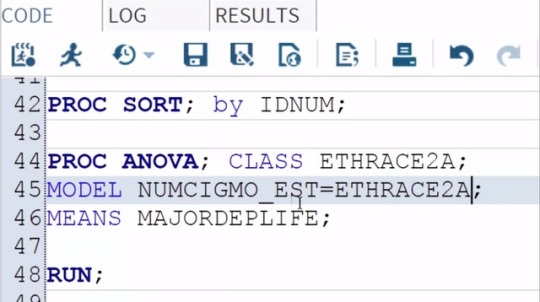
Data Analysis Tool: Assignment_1

In order to conduct post hoc paired comparisons in the context of Mironova. 

Examining the association between ethnicity and number of cigarettes smoked 

per month among young adult smokers, I'm going to use the Duncan Test. 

To do this, all I need to do is add a slash and 

the word Duncan at the end of my MEANS statement. 

And then save and run my program. 

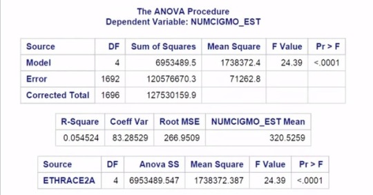
Here are the Proc ANOVA results with Duncan Post Hoc Test. 

The top of our results looks the same as in our original test. 

The F value or F statistic is 24.4 and 

it's significant at the P < 0.0001 level. 

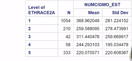
However, if we scroll down, we see a new table displaying the results of the paired 

comparisons conducted by the Duncan Multiple Range Test.