bbadland

[bbadland]

Module 10

A1. Regression analysis of cystfibr:

In the output of our regression model, we see the strongest relationship between pemax and age, with an inverse relationship between age and maximum expiratory pressure. As age increases by one year, pemax decreases by 3.2 units, adjusted for the other terms in the model. Additionally, a positive relationship exists between weight and pemax, with the increase of an individual's weight being tied to maximum expiratory pressure. Our small relational effect in the regression model is fev1, or forced expiratory volume. Every 1.0 unit increase of pemax corresponds with a 1.088 unit increase of fev1 (again, adjusted for the other terms in the model), indicating an extremely small positive relationship between variables.

ANOVA analysis of cystfibr:

Our ANOVA output confirms a significant relationship between age and pemax, with a F-value of 18.43 and and p-value of 0.00035. When analyzing this data with the results of the regression model, we can safely theorize that pemax has a significant inverse relationship with an individual's age. While our regression model indicates an increase of pemax associated with an increase of weight, we fail to reject the null hypothesis with our ANOVA results, as the p-value is well above a significance level of 0.05. What's most interesting to me is the relationship between fev1 and pemax: the regression model indicated a very slight positive relationship between those two variables, and the ANOVA results show that the relationship is unlikely to be caused by chance. Therefore, we can say that fev1 and pemax have a statistical relationship, even though the actual effect they have is quite small.

B1. After running a regression model on the abdominal diameter and biparietal diameter variables, we see their respective coefficients are 2.237 and 3.332.

When running a combined model the coefficient for ad decreases to 1.467, while the coefficient for bpd also decreases to 1.552.

However, as stated, the sum of their coefficients are very close to 3. By using the combined model, both dimensions can be used to accurately estimate a birth weight. While each single variable fit produces a satisfactory regression coefficient, we have better control of the prediction by using a model that combines both dimensions.

B2. Yes, I believe using both dimensions can prove to do so. As stated before, the sum of coefficients are very close to 3 when using the combined model. In order to give further proof to the utility of the combined model, I ran an R-squared test for each model.

The R-squared value for ad is 0.7959, 0.7221 for bpd, and 0.8583 for our combined model. Comparing these statistics, we can see that the combined model is the most valuable fit for predicting birth weight. Moving beyond a statistical standpoint, using both dimensions in our model results in a more accurate representation of the volume, and therefore the weight, of the newborn.

B3. Log transformation can be used to "smooth" out data to ease calculation and interpretation. From Rohit Farmer at dataalltheway.com:

By log-transforming this data, we can modify it to reveal a normal distribution. It's also useful when dealing with a dataset with values that are orders of magnitudes away from each other, as a log transformation can be used to normalize this data.

[bbadland]

Module 9

A1. Here we have a one-way table for purchased:

A2. Two-way table for country and purchased:

B1. Here is the mtcars dataframe with added margins:

B2. Here is the proportional weight table of mtcars for each value:

[bbadland]

Assignment 8

A.

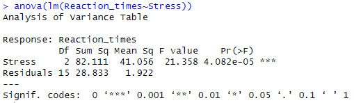
Upon running the ANOVA test in R, for stress levels and drug reaction times, we can see that there are 2 degrees of freedom (as df = N - 1 and there are three variables). The sum of squares (or variation, Sum Sq) is 82.11 between stress groups and 28.83 within stress groups, meaning that reaction times varies more against other stress levels than within the same stress levels. The Mean Square (or average variance, Mean Sq) of reaction time is 41.06 between stress levels and 1.92 within stress levels. The F-Statistic (test statistic of variation within groups vs against groups, F value) is high, meaning that there is more variation in reaction time between stress levels than within stress levels. The p-value (probability of these results occurring by chance, Pr(>F)) is extremely low at 0.00004082, which is significantly lower than a testing value of 0.05. Using this data, we can determine that it is extremely statistically likely that stress levels and drug reaction times are in some way related.

B1.

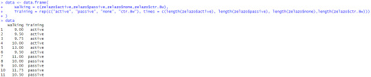
First, I combined the zelazo data (which I realized halfway through B1 is in fact data from a study cited in the textbook and not seemingly random variables and numbers) under the relevant "Training" and "Walking" columns to prepare it for testing.

Then I gave up trying to calculate a t-test within the data frame I created for the ANOVA test so I just ran it normally.

The negative t-statistic means that the mean of the group of actively trained children is smaller than the mean of the group of passively trained children. Our p-value is greater than 0.05, so we fail to reject that there is a difference between passively and actively trained children.

However, when running the t-test comparing the actively trained children to the control group that received no training and only a single test:

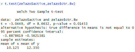
There is an even more significant difference in the t-statistic when comparing active and passively trained children. Additionally, the p-value is lower than the significance threshold of 0.05.

It's important to note within the context of the experiment while that the control group (ctr.8w) did not receive any training, they were only tested once throughout the experiment. On the other hand, the "none" group did not receive any training but were repeatedly tested. When testing the active group vs the "none" group, the p-value is 0.094, above a significant value of 0.05.

B2.

I used a one-way ANOVA test on this dataset. Variation between training groups was greater than the variation within stress groups. Our F-statistic is also relatively low, indicating not much variation between groups. Finally, our p-value is 0.1285, surpassing a significance level of both 0.05 and 0.10.

[bbadland]

Module 6

A1. 11.8

A2. 8, 11

A3. xbar = 9.5, sd = 2.12

A4. While the population mean is much higher than the sample mean, the standard deviation remained the same value. 

B1. The distribution is expected to be normal if both np and nq are greater than or equal to 5, which is true, meaning that sample proportion p has approximately a normal distribution. Since n * p = 95 and n * q = 5, we can hold it to be true that this fits a normal distribution. 

B2. Sample size n is already at the lowest possible sampling distribution for which p is approximately normal, as any size lower than this would result in nq being lower than 5. 

C1. The sample function randomly selects from a vector and is best used when drawing data from a population. When making a coin tossing simulation, the better fit is rbinom, as its function generates numbers from a binomial distribution.

[bbadland]

Assignment 5

Question A.

A1: The null hypothesis, or H(0), is that the machine is working correctly with a mean breaking strength of 70lbs. The alternative hypothesis, or H(A), is that the machine is not working correctly, and the mean breaking strength is a different value than 70lbs. 

A2: Using a 0.05 level of significance, we fail to reject H(0), as the p-value is 0.072. Therefore, there is no evidence that the machine is not meeting manufacturer specifications. 

A3: The p-value is 0.072, which is greater than 0.05, leading us to fail to reject H(0). This means that the probability of the result occurring by chance is 7.2%. In order to reject H(0), we would need a statistically significant result below 0.05. 

A4: If the standard deviation was 1.75, we would reject the null hypothesis, as the p-value would be below 0.05. This would mean that there is statistically significant evidence that the machine is not meeting manufacturer specifications.

A5: If the sample mean were just slightly lower at 69lbs and the standard deviation remaining at 3.5lbs, we would reject the null hypothesis. The p-value becomes 0.045, giving statistically significant evidence that the machine is not meeting manufacturer specifications. 

Question B.

The 95% confidence interval estimate is from 83.04 to 86.96.

Question C.

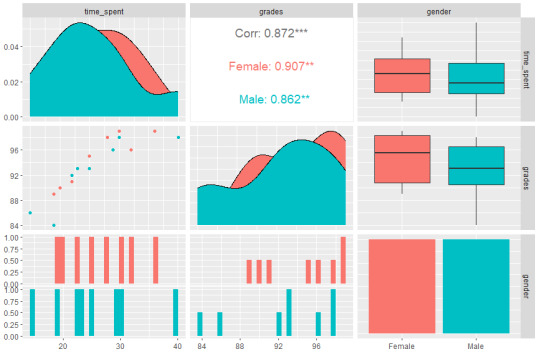
C1: Pearson’s correlation coefficient between time spent studying to grades is 0.91 for girls and 0.86 for boys.

C2: 

[bbadland]

Assignment 2

The function call myMean returns the mean of the data vector of a given variable. Calling the function for the variable assignment2 results in a mean of 18.66667. The syntax of the myMean function returns the sum of a data set divided by the length of the data set, thus calculating the average of the data vector. The curly brackets identify what specifically the myMean function performs.

[bbadland]

First-Day Assignment

Howdy,

My name is Beckett Badland, and I have been a student here at USF since 2019. My interest in data science began in the field of geography, where I gained experience in building geodatabases and processing large datasets using Python, R, VBA, and GlobalMapper. In 2023, I decided to switch to part-time schooling and begin a career in commercial aviation maintenance. My goal is to combine my passion for aviation and data science to expand on existing methods of identifying maintenance trends to increase aircraft reliability and reduce costly downtime. Currently, I work at a base hangar in Boise maintaining aircraft at the largest regional airline in North America.