
Statistics
We looked inside some of the posts by datasciencewithmohsin and here's what we found interesting.
Average Info
Notes Per Post
52
Likes Per Post
22
Reblog Per Post
30
Reply Per Post
0
Time Between Posts
1 day
Number of Posts By Type
Text
17
Last Seen Tumblr Blogs


Fun Fact
The Tumblr app for Google Glass was released on May 16, 2013.
Text
Beginner’s Guide to Ridge Regression in Machine Learning
Introduction
Regression analysis is a fundamental technique in machine learning, used to predict a dependent variable based on one or more independent variables. However, traditional regression methods, such as simple linear regression, can struggle to deal with multicollinearity (high correlation between predictors). This is where ridge regression comes in handy.
Ridge regression is an advanced form of linear regression that reduces overfitting by adding a penalty term to the model. In this article, we will cover what ridge regression is, why it is important, how it works, its assumptions, and how to implement it using Python.
What is Ridge Regression?
Ridge regression is a type of regularization technique that modifies the linear
click here to read more
https://datacienceatoz.blogspot.com/2025/02/a-beginners-guide-to-ridge-regression.html
4 notes
·
View notes
Text
Understanding Outliers in Machine Learning and Data Science

In machine learning and data science, an outlier is like a misfit in a dataset. It's a data point that stands out significantly from the rest of the data. Sometimes, these outliers are errors, while other times, they reveal something truly interesting about the data. Either way, handling outliers is a crucial step in the data preprocessing stage. If left unchecked, they can skew your analysis and even mess up your machine learning models.
In this article, we will dive into:
1. What outliers are and why they matter.
2. How to detect and remove outliers using the Interquartile Range (IQR) method.
3. Using the Z-score method for outlier detection and removal.
4. How the Percentile Method and Winsorization techniques can help handle outliers.
This guide will explain each method in simple terms with Python code examples so that even beginners can follow along.
1. What Are Outliers?
An outlier is a data point that lies far outside the range of most other values in your dataset. For example, in a list of incomes, most people might earn between $30,000 and $70,000, but someone earning $5,000,000 would be an outlier.
Why Are Outliers Important?
Outliers can be problematic or insightful:
Problematic Outliers: Errors in data entry, sensor faults, or sampling issues.
Insightful Outliers: They might indicate fraud, unusual trends, or new patterns.
Types of Outliers
1. Univariate Outliers: These are extreme values in a single variable.
Example: A temperature of 300°F in a dataset about room temperatures.
2. Multivariate Outliers: These involve unusual combinations of values in multiple variables.
Example: A person with an unusually high income but a very low age.
3. Contextual Outliers: These depend on the context.
Example: A high temperature in winter might be an outlier, but not in summer.
2. Outlier Detection and Removal Using the IQR Method
The Interquartile Range (IQR) method is one of the simplest ways to detect outliers. It works by identifying the middle 50% of your data and marking anything that falls far outside this range as an outlier.
Steps:
1. Calculate the 25th percentile (Q1) and 75th percentile (Q3) of your data.
2. Compute the IQR:
{IQR} = Q3 - Q1
Q1 - 1.5 \times \text{IQR}
Q3 + 1.5 \times \text{IQR} ] 4. Anything below the lower bound or above the upper bound is an outlier.
Python Example:
import pandas as pd
# Sample dataset
data = {'Values': [12, 14, 18, 22, 25, 28, 32, 95, 100]}
df = pd.DataFrame(data)
# Calculate Q1, Q3, and IQR
Q1 = df['Values'].quantile(0.25)
Q3 = df['Values'].quantile(0.75)
IQR = Q3 - Q1
# Define the bounds
lower_bound = Q1 - 1.5 * IQR
upper_bound = Q3 + 1.5 * IQR
# Identify and remove outliers
outliers = df[(df['Values'] < lower_bound) | (df['Values'] > upper_bound)]
print("Outliers:\n", outliers)
filtered_data = df[(df['Values'] >= lower_bound) & (df['Values'] <= upper_bound)]
print("Filtered Data:\n", filtered_data)
Key Points:
The IQR method is great for univariate datasets.
It works well when the data isn’t skewed or heavily distributed.
3. Outlier Detection and Removal Using the Z-Score Method
The Z-score method measures how far a data point is from the mean, in terms of standard deviations. If a Z-score is greater than a certain threshold (commonly 3 or -3), it is considered an outlier.
Formula:
Z = \frac{(X - \mu)}{\sigma}
is the data point,
is the mean of the dataset,
is the standard deviation.
Python Example:
import numpy as np
# Sample dataset
data = {'Values': [12, 14, 18, 22, 25, 28, 32, 95, 100]}
df = pd.DataFrame(data)
# Calculate mean and standard deviation
mean = df['Values'].mean()
std_dev = df['Values'].std()
# Compute Z-scores
df['Z-Score'] = (df['Values'] - mean) / std_dev
# Identify and remove outliers
threshold = 3
outliers = df[(df['Z-Score'] > threshold) | (df['Z-Score'] < -threshold)]
print("Outliers:\n", outliers)
filtered_data = df[(df['Z-Score'] <= threshold) & (df['Z-Score'] >= -threshold)]
print("Filtered Data:\n", filtered_data)
Key Points:
The Z-score method assumes the data follows a normal distribution.
It may not work well with skewed datasets.
4. Outlier Detection Using the Percentile Method and Winsorization
Percentile Method:
In the percentile method, we define a lower percentile (e.g., 1st percentile) and an upper percentile (e.g., 99th percentile). Any value outside this range is treated as an outlier.
Winsorization:
Winsorization is a technique where outliers are not removed but replaced with the nearest acceptable value.
Python Example:
from scipy.stats.mstats import winsorize
import numpy as np
Sample data
data = [12, 14, 18, 22, 25, 28, 32, 95, 100]
Calculate percentiles
lower_percentile = np.percentile(data, 1)
upper_percentile = np.percentile(data, 99)
Identify outliers
outliers = [x for x in data if x < lower_percentile or x > upper_percentile]
print("Outliers:", outliers)
# Apply Winsorization
winsorized_data = winsorize(data, limits=[0.01, 0.01])
print("Winsorized Data:", list(winsorized_data))
Key Points:
Percentile and Winsorization methods are useful for skewed data.
Winsorization is preferred when data integrity must be preserved.
Final Thoughts
Outliers can be tricky, but understanding how to detect and handle them is a key skill in machine learning and data science. Whether you use the IQR method, Z-score, or Wins
orization, always tailor your approach to the specific dataset you’re working with.
By mastering these techniques, you’ll be able to clean your data effectively and improve the accuracy of your models.
4 notes
·
View notes
Text
What is Gradient Descent?
Gradient descent is an efficient first-order optimization algorithm for finding a differentiable function's global or local minimum. It estimates the values of parameters or coefficients that minimize a cost function.
The gradient descent method has proved to be especially useful as it can be adopted in spaces of any number of dimensions. The gradient descent method can be used when parameters cannot be calculated analytically and is a good choice for the differentiable cost function.
https://datacienceatoz.blogspot.com/2025/01/the-z-guide-to-gradient-descent.html
#datascience #machinelearning #post #gardientdescent

3 notes
·
View notes
Text
Beginner’s Guide to Ridge Regression in Machine Learning
Introduction
Regression analysis is a fundamental technique in machine learning, used to predict a dependent variable based on one or more independent variables. However, traditional regression methods, such as simple linear regression, can struggle to deal with multicollinearity (high correlation between predictors). This is where ridge regression comes in handy.
Ridge regression is an advanced form of linear regression that reduces overfitting by adding a penalty term to the model. In this article, we will cover what ridge regression is, why it is important, how it works, its assumptions, and how to implement it using Python.
What is Ridge Regression?
Ridge regression is a type of regularization technique that modifies the linear
click here to read more
https://datacienceatoz.blogspot.com/2025/02/a-beginners-guide-to-ridge-regression.html
4 notes
·
View notes
Text
Beginner’s Guide to Ridge Regression in Machine Learning
Introduction
Regression analysis is a fundamental technique in machine learning, used to predict a dependent variable based on one or more independent variables. However, traditional regression methods, such as simple linear regression, can struggle to deal with multicollinearity (high correlation between predictors). This is where ridge regression comes in handy.
Ridge regression is an advanced form of linear regression that reduces overfitting by adding a penalty term to the model. In this article, we will cover what ridge regression is, why it is important, how it works, its assumptions, and how to implement it using Python.
What is Ridge Regression?
Ridge regression is a type of regularization technique that modifies the linear
click here to read more
https://datacienceatoz.blogspot.com/2025/02/a-beginners-guide-to-ridge-regression.html
#artificial intelligence#bigdata#machinelearning#books#programming#machine learning#skills#python#science#big data
4 notes
·
View notes
Text
Beginner’s Guide to Ridge Regression in Machine Learning
Introduction
Regression analysis is a fundamental technique in machine learning, used to predict a dependent variable based on one or more independent variables. However, traditional regression methods, such as simple linear regression, can struggle to deal with multicollinearity (high correlation between predictors). This is where ridge regression comes in handy.
Ridge regression is an advanced form of linear regression that reduces overfitting by adding a penalty term to the model. In this article, we will cover what ridge regression is, why it is important, how it works, its assumptions, and how to implement it using Python.
What is Ridge Regression?
Ridge regression is a type of regularization technique that modifies the linear
click here to read more
https://datacienceatoz.blogspot.com/2025/02/a-beginners-guide-to-ridge-regression.html
#artificial intelligence#bigdata#books#machine learning#machinelearning#programming#python#science#skills#big data
4 notes
·
View notes
Text
What is Gradient Descent?
Gradient descent is an efficient first-order optimization algorithm for finding a differentiable function's global or local minimum. It estimates the values of parameters or coefficients that minimize a cost function.
The gradient descent method has proved to be especially useful as it can be adopted in spaces of any number of dimensions. The gradient descent method can be used when parameters cannot be calculated analytically and is a good choice for the differentiable cost function.
https://datacienceatoz.blogspot.com/2025/01/the-z-guide-to-gradient-descent.html
#datascience #machinelearning #post #gardientdescent
#artificial intelligence#bigdata#machine learning#books#programming#machinelearning#skills#python#science#big data
3 notes
·
View notes
Text
Understanding Outliers in Machine Learning and Data Science
In machine learning and data science, an outlier is like a misfit in a dataset. It's a data point that stands out significantly from the rest of the data. Sometimes, these outliers are errors, while other times, they reveal something truly interesting about the data. Either way, handling outliers is a crucial step in the data preprocessing stage. If left unchecked, they can skew your analysis and even mess up your machine learning models.
In this article, we will dive into:
1. What outliers are and why they matter.
2. How to detect and remove outliers using the Interquartile Range (IQR) method.
3. Using the Z-score method for outlier detection and removal.
4. How the Percentile Method and Winsorization techniques can help handle outliers.
This guide will explain each method in simple terms with Python code examples so that even beginners can follow along.
1. What Are Outliers?
An outlier is a data point that lies far outside the range of most other values in your dataset. For example, in a list of incomes, most people might earn between $30,000 and $70,000, but someone earning $5,000,000 would be an outlier.
Why Are Outliers Important?
Outliers can be problematic or insightful:
Problematic Outliers: Errors in data entry, sensor faults, or sampling issues.
Insightful Outliers: They might indicate fraud, unusual trends, or new patterns.
Types of Outliers
1. Univariate Outliers: These are extreme values in a single variable.
Example: A temperature of 300°F in a dataset about room temperatures.
2. Multivariate Outliers: These involve unusual combinations of values in multiple variables.
Example: A person with an unusually high income but a very low age.
3. Contextual Outliers: These depend on the context.
Example: A high temperature in winter might be an outlier, but not in summer.
2. Outlier Detection and Removal Using the IQR Method
The Interquartile Range (IQR) method is one of the simplest ways to detect outliers. It works by identifying the middle 50% of your data and marking anything that falls far outside this range as an outlier.
Steps:
1. Calculate the 25th percentile (Q1) and 75th percentile (Q3) of your data.
2. Compute the IQR:
{IQR} = Q3 - Q1
Q1 - 1.5 \times \text{IQR}
Q3 + 1.5 \times \text{IQR} ] 4. Anything below the lower bound or above the upper bound is an outlier.
Python Example:
import pandas as pd
# Sample dataset
data = {'Values': [12, 14, 18, 22, 25, 28, 32, 95, 100]}
df = pd.DataFrame(data)
# Calculate Q1, Q3, and IQR
Q1 = df['Values'].quantile(0.25)
Q3 = df['Values'].quantile(0.75)
IQR = Q3 - Q1
# Define the bounds
lower_bound = Q1 - 1.5 * IQR
upper_bound = Q3 + 1.5 * IQR
# Identify and remove outliers
outliers = df[(df['Values'] < lower_bound) | (df['Values'] > upper_bound)]
print("Outliers:\n", outliers)
filtered_data = df[(df['Values'] >= lower_bound) & (df['Values'] <= upper_bound)]
print("Filtered Data:\n", filtered_data)
Key Points:
The IQR method is great for univariate datasets.
It works well when the data isn’t skewed or heavily distributed.
3. Outlier Detection and Removal Using the Z-Score Method
The Z-score method measures how far a data point is from the mean, in terms of standard deviations. If a Z-score is greater than a certain threshold (commonly 3 or -3), it is considered an outlier.
Formula:
Z = \frac{(X - \mu)}{\sigma}
is the data point,
is the mean of the dataset,
is the standard deviation.
Python Example:
import numpy as np
# Sample dataset
data = {'Values': [12, 14, 18, 22, 25, 28, 32, 95, 100]}
df = pd.DataFrame(data)
# Calculate mean and standard deviation
mean = df['Values'].mean()
std_dev = df['Values'].std()
# Compute Z-scores
df['Z-Score'] = (df['Values'] - mean) / std_dev
# Identify and remove outliers
threshold = 3
outliers = df[(df['Z-Score'] > threshold) | (df['Z-Score'] < -threshold)]
print("Outliers:\n", outliers)
filtered_data = df[(df['Z-Score'] <= threshold) & (df['Z-Score'] >= -threshold)]
print("Filtered Data:\n", filtered_data)
Key Points:
The Z-score method assumes the data follows a normal distribution.
It may not work well with skewed datasets.
4. Outlier Detection Using the Percentile Method and Winsorization
Percentile Method:
In the percentile method, we define a lower percentile (e.g., 1st percentile) and an upper percentile (e.g., 99th percentile). Any value outside this range is treated as an outlier.
Winsorization:
Winsorization is a technique where outliers are not removed but replaced with the nearest acceptable value.
Python Example:
from scipy.stats.mstats import winsorize
import numpy as np
Sample data
data = [12, 14, 18, 22, 25, 28, 32, 95, 100]
Calculate percentiles
lower_percentile = np.percentile(data, 1)
upper_percentile = np.percentile(data, 99)
Identify outliers
outliers = [x for x in data if x < lower_percentile or x > upper_percentile]
print("Outliers:", outliers)
# Apply Winsorization
winsorized_data = winsorize(data, limits=[0.01, 0.01])
print("Winsorized Data:", list(winsorized_data))
Key Points:
Percentile and Winsorization methods are useful for skewed data.
Winsorization is preferred when data integrity must be preserved.
Final Thoughts
Outliers can be tricky, but understanding how to detect and handle them is a key skill in machine learning and data science. Whether you use the IQR method, Z-score, or Wins
orization, always tailor your approach to the specific dataset you’re working with.
By mastering these techniques, you’ll be able to clean your data effectively and improve the accuracy of your models.
4 notes
·
View notes
Text

Feature Engineering in Machine Learning: A Beginner's Guide
Feature Engineering in Machine Learning: A Beginner's Guide
Feature engineering is one of the most critical aspects of machine learning and data science. It involves preparing raw data, transforming it into meaningful features, and optimizing it for use in machine learning models. Simply put, it’s all about making your data as informative and useful as possible.
In this article, we’re going to focus on feature transformation, a specific type of feature engineering. We’ll cover its types in detail, including:
1. Missing Value Imputation
2. Handling Categorical Data
3. Outlier Detection
4. Feature Scaling
Each topic will be explained in a simple and beginner-friendly way, followed by Python code examples so you can implement these techniques in your projects.
What is Feature Transformation?
Feature transformation is the process of modifying or optimizing features in a dataset. Why? Because raw data isn’t always machine-learning-friendly. For example:
Missing data can confuse your model.
Categorical data (like colors or cities) needs to be converted into numbers.
Outliers can skew your model’s predictions.
Different scales of features (e.g., age vs. income) can mess up distance-based algorithms like k-NN.
1. Missing Value Imputation
Missing values are common in datasets. They can happen due to various reasons: incomplete surveys, technical issues, or human errors. But machine learning models can’t handle missing data directly, so we need to fill or "impute" these gaps.
Techniques for Missing Value Imputation
1. Dropping Missing Values: This is the simplest method, but it’s risky. If you drop too many rows or columns, you might lose important information.
2. Mean, Median, or Mode Imputation: Replace missing values with the column’s mean (average), median (middle value), or mode (most frequent value).
3. Predictive Imputation: Use a model to predict the missing values based on other features.
Python Code Example:
import pandas as pd
from sklearn.impute import SimpleImputer
# Example dataset
data = {'Age': [25, 30, None, 22, 28], 'Salary': [50000, None, 55000, 52000, 58000]}
df = pd.DataFrame(data)
# Mean imputation
imputer = SimpleImputer(strategy='mean')
df['Age'] = imputer.fit_transform(df[['Age']])
df['Salary'] = imputer.fit_transform(df[['Salary']])
print("After Missing Value Imputation:\n", df)
Key Points:
Use mean/median imputation for numeric data.
Use mode imputation for categorical data.
Always check how much data is missing—if it’s too much, dropping rows might be better.
2. Handling Categorical Data
Categorical data is everywhere: gender, city names, product types. But machine learning algorithms require numerical inputs, so you’ll need to convert these categories into numbers.
Techniques for Handling Categorical Data
1. Label Encoding: Assign a unique number to each category. For example, Male = 0, Female = 1.
2. One-Hot Encoding: Create separate binary columns for each category. For instance, a “City” column with values [New York, Paris] becomes two columns: City_New York and City_Paris.
3. Frequency Encoding: Replace categories with their occurrence frequency.
Python Code Example:
from sklearn.preprocessing import LabelEncoder
import pandas as pd
# Example dataset
data = {'City': ['New York', 'London', 'Paris', 'New York', 'Paris']}
df = pd.DataFrame(data)
# Label Encoding
label_encoder = LabelEncoder()
df['City_LabelEncoded'] = label_encoder.fit_transform(df['City'])
# One-Hot Encoding
df_onehot = pd.get_dummies(df['City'], prefix='City')
print("Label Encoded Data:\n", df)
print("\nOne-Hot Encoded Data:\n", df_onehot)
Key Points:
Use label encoding when categories have an order (e.g., Low, Medium, High).
Use one-hot encoding for non-ordered categories like city names.
For datasets with many categories, one-hot encoding can increase complexity.
3. Outlier Detection
Outliers are extreme data points that lie far outside the normal range of values. They can distort your analysis and negatively affect model performance.
Techniques for Outlier Detection
1. Interquartile Range (IQR): Identify outliers based on the middle 50% of the data (the interquartile range).
IQR = Q3 - Q1
[Q1 - 1.5 \times IQR, Q3 + 1.5 \times IQR]
2. Z-Score: Measures how many standard deviations a data point is from the mean. Values with Z-scores > 3 or < -3 are considered outliers.
Python Code Example (IQR Method):
import pandas as pd
# Example dataset
data = {'Values': [12, 14, 18, 22, 25, 28, 32, 95, 100]}
df = pd.DataFrame(data)
# Calculate IQR
Q1 = df['Values'].quantile(0.25)
Q3 = df['Values'].quantile(0.75)
IQR = Q3 - Q1
# Define bounds
lower_bound = Q1 - 1.5 * IQR
upper_bound = Q3 + 1.5 * IQR
# Identify and remove outliers
outliers = df[(df['Values'] < lower_bound) | (df['Values'] > upper_bound)]
print("Outliers:\n", outliers)
filtered_data = df[(df['Values'] >= lower_bound) & (df['Values'] <= upper_bound)]
print("Filtered Data:\n", filtered_data)
Key Points:
Always understand why outliers exist before removing them.
Visualization (like box plots) can help detect outliers more easily.
4. Feature Scaling
Feature scaling ensures that all numerical features are on the same scale. This is especially important for distance-based models like k-Nearest Neighbors (k-NN) or Support Vector Machines (SVM).
Techniques for Feature Scaling
1. Min-Max Scaling: Scales features to a range of [0, 1].
X' = \frac{X - X_{\text{min}}}{X_{\text{max}} - X_{\text{min}}}
2. Standardization (Z-Score Scaling): Centers data around zero with a standard deviation of 1.
X' = \frac{X - \mu}{\sigma}
3. Robust Scaling: Uses the median and IQR, making it robust to outliers.
Python Code Example:
from sklearn.preprocessing import MinMaxScaler, StandardScaler
import pandas as pd
# Example dataset
data = {'Age': [25, 30, 35, 40, 45], 'Salary': [20000, 30000, 40000, 50000, 60000]}
df = pd.DataFrame(data)
# Min-Max Scaling
scaler = MinMaxScaler()
df_minmax = pd.DataFrame(scaler.fit_transform(df), columns=df.columns)
# Standardization
scaler = StandardScaler()
df_standard = pd.DataFrame(scaler.fit_transform(df), columns=df.columns)
print("Min-Max Scaled Data:\n", df_minmax)
print("\nStandardized Data:\n", df_standard)
Key Points:
Use Min-Max Scaling for algorithms like k-NN and neural networks.
Use Standardization for algorithms that assume normal distributions.
Use Robust Scaling when your data has outliers.
Final Thoughts
Feature transformation is a vital part of the data preprocessing pipeline. By properly imputing missing values, encoding categorical data, handling outliers, and scaling features, you can dramatically improve the performance of your machine learning models.
Summary:
Missing value imputation fills gaps in your data.
Handling categorical data converts non-numeric features into numerical ones.
Outlier detection ensures your dataset isn’t skewed by extreme values.
Feature scaling standardizes feature ranges for better model performance.
Mastering these techniques will help you build better, more reliable machine learning models.
1 note
·
View note
Text

Feature Construction and Feature Splitting in Machine Learning
Feature engineering is one of the most important parts of the machine learning process. It helps improve the performance of models by modifying and optimizing the data. In this article, we’ll focus on two crucial feature engineering techniques: feature construction and feature splitting. Both are beginner-friendly and can significantly improve the quality of your dataset.
Let’s break it down into a simple, list-based structure to make it easy to follow.
1. Feature Construction
What is Feature Construction?
Feature construction is the process of creating new features from raw data or combining existing ones to provide better insights for a machine learning model.
For example:
From a Date column, we can construct features like Year, Month, or Day.
For a Price column, you can create a Price_Per_Unit feature by dividing the price by the number of units.
Why is Feature Construction Important?
1. Improves Accuracy: New features often capture hidden patterns in the data.
2. Simplifies Relationships: Some models work better when data is transformed into simpler relationships.
3. Handles Missing Information: Constructed features can sometimes fill gaps in the dataset.
Techniques for Feature Construction
1. Date Feature Construction
Extract components like year, month, day, or even day of the week from date columns.
Helps analyze trends or seasonality.
2. Mathematical Transformations
Create new features using arithmetic operations.
Example: If you have Length and Width, construct an Area = Length × Width feature.
3. Text Feature Construction
Extract features like word count, average word length, or even sentiment from text data.
4. Polynomial Features
Generate interaction terms or powers of numerical features to capture non-linear relationships.
Example: X1^2, X1 * X2.
Python Code for Feature Construction
Example 1: Constructing Features from Dates
import pandas as pd
# Sample dataset
data = {'date': ['2023-01-01', '2023-03-10', '2023-07-20']}
df = pd.DataFrame(data)
# Convert to datetime
df['date'] = pd.to_datetime(df['date'])
# Construct new features
df['year'] = df['date'].dt.year
df['month'] = df['date'].dt.month
df['day_of_week'] = df['date'].dt.dayofweek
df['is_weekend'] = df['day_of_week'].apply(lambda x: 1 if x >= 5 else 0)
print(df)
Example 2: Creating Polynomial Features
from sklearn.preprocessing import PolynomialFeatures
import pandas as pd
# Sample dataset
data = {'X1': [2, 3, 5], 'X2': [4, 6, 8]}
df = pd.DataFrame(data)
# Generate polynomial features
poly = PolynomialFeatures(degree=2, include_bias=False)
poly_features = poly.fit_transform(df)
# Convert to DataFrame
poly_df = pd.DataFrame(poly_features, columns=poly.get_feature_names_out(['X1', 'X2']))
print(poly_df)
for more read click here https://datacienceatoz.blogspot.com/2025/01/feature-construction-and-feature.html
#datascince #machinelearnings #data #science
1 note
·
View note
Text
Regression metrics in machine learning

Regression metrics help us evaluate the performance of regression models in machine learning. For beginners, understanding these parameters is important for model selection and optimization. In this article, we will focus on the important regression metrics: MAE, MSE, RMSE, R² score, and adjusted R² score.
Each section is written in list format for better clarity and understanding.
1. Mean Absolute Error (MAE)
MAE calculates the average of absolute differences between predicted and actual values.
formula:
Important points:
1. Easy to understand: MAE is easy to understand and calculate.
2. Same unit as the target variable: The errors are in the same unit as the target variable.
3. Not sensitive to outliers: Large errors do not affect MAE as much as they do MSE.
Use cases:
When you need a simple and descriptive metric for error measurement.
Python code:
import mean_absolute_error from sklearn.metrics
# Actual and projected values
y_true = [50, 60, 70, 80, 90]
y_pred = [48, 62, 69, 78, 91]
# Calculate the MAE
mae = mean_absolute_error (y_true, y_pred)
print("Mean Absolute Error (MAE):", mae)
2. Mean Squared Error (MSE)
MSE calculates the average of the squared differences between predicted and actual values.
formula:
Important points:
1. Punishes big mistakes: Square mistakes increase their impact.
2. Optimization in general: widely used for model training.
3. Units are squared: Errors are in squared units of the target variable, which can be difficult to interpret.
Use cases:
Useful when you want to punish big mistakes.
Python code:
import mean_squared_error from sklearn.metrics
# Calculate the MSE
mse = mean_squared_error(y_true, y_pred)
print("Mean Squared Error (MSE): "mse)
3. Root Mean Squared Error (RMSE)
Description:
RMSE is the square root of MSE and provides a more descriptive error metric.
Important points
1. Same unit target variable: Easier to interpret than MSE.
2. Sensitive to outliers: Like MSE, RMSE penalizes large errors.
Use cases:
When you need an interpretable error measure that considers large deviations.
Python code:
import np as numpy
# Calculate the RMSE
rmse = np.sqrt(mse)
print("Root Mean Squared Error (RMSE):", rmse)
4. R-squared (R²) score
R² measures how much variance in the target variable is explained by the model.
formula:
Important points:
1. Range: R² ranges from 0 to 1, with 1 being a perfect fit.
2. Negative values: A negative R² indicates the model is worse at predicting the mean.
3. Explains variance: Higher values mean the model explains more variance.
Use cases:
Estimate the overall goodness of fit of the regression model.
Python code:
import r2_score from sklearn.metrics;
# Calculate the R² score
r2 = r2_score(y_true, y_pred)
print("R-Squared (R²) score:", r2);
5. Adjusted R-Square
Description:
Adjusted R² Adjusts the R² value by the number of predictors in the model.
formula:
: number of observations
: number of predictors
Important points:
1. Better for multiple predictors: Penalizes models with irrelevant features.
2. Can decrease: Unlike R², adjusted R² can decrease when adding unrelated predictors.
Use cases:
Comparing models with different statistics.
Python code:
# function to calculate the adjusted R²
def adjusted_r2(r2, n, p):
Returns 1 - ((1 - r2) * (n - 1) / (n - p - 1))
# Example calculations
n = lane(y_true)
p = 1 # Number of predictors
adj_r2 = adjusted_r2 (r2, n, p)
print("adjusted r-squared:", adj_r2);
Comparison of metrics
result
Understanding these regression metrics helps build, evaluate, and compare models effectively. Each metric serves a specific purpose:
1. Use MAE for simple and robust error measurement.
2. Opt for MSE or RMSE when it is important to penalize large errors.
3. Evaluate the performance of the model
e using R².
4. Prefer adjusted R² for models with multiple characteristicjs.
These metrics are fundamental to any data scientist or machine learning engineer aiming to build accurate and reliable regression models.
1 note
·
View note
Text
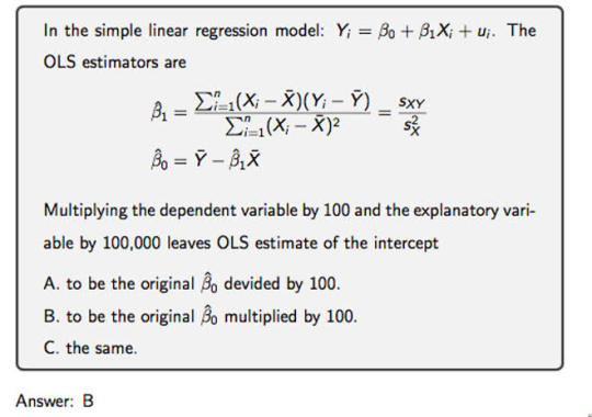
Simple Linear Regression in Data Science and machine learning
Simple linear regression is one of the most important techniques in data science and machine learning. It is the foundation of many statistical and machine learning models. Even though it is simple, its concepts are widely applicable in predicting outcomes and understanding relationships between variables.
This article will help you learn about:
1. What is simple linear regression and why it matters.
2. The step-by-step intuition behind it.
3. The math of finding slope() and intercept().
4. Simple linear regression coding using Python.
5. A practical real-world implementation.
If you are new to data science or machine learning, don’t worry! We will keep things simple so that you can follow along without any problems.
What is simple linear regression?
Simple linear regression is a method to model the relationship between two variables:
1. Independent variable (X): The input, also called the predictor or feature.
2. Dependent Variable (Y): The output or target value we want to predict.
The main purpose of simple linear regression is to find a straight line (called the regression line) that best fits the data. This line minimizes the error between the actual and predicted values.
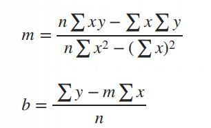
The mathematical equation for the line is:
Y = mX + b
: The predicted values.
: The slope of the line (how steep it is).
: The intercept (the value of when).
Why use simple linear regression?
click here to read more https://datacienceatoz.blogspot.com/2025/01/simple-linear-regression-in-data.html
6 notes
·
View notes
Text

A Beginner's Guide to Principal Component Analysis (PCA) in Data Science and Machine Learning
Principal Component Analysis (PCA) is one of the most important techniques for dimensionality reduction in machine learning and data science. It allows us to simplify datasets, making them easier to work with while retaining as much valuable information as possible. PCA has become a go-to method for preprocessing high-dimensional data.
Click here to read more
3 notes
·
View notes
Text
Simple Linear Regression in Data Science and machine learning
Simple linear regression is one of the most important techniques in data science and machine learning. It is the foundation of many statistical and machine learning models. Even though it is simple, its concepts are widely applicable in predicting outcomes and understanding relationships between variables.
This article will help you learn about:
1. What is simple linear regression and why it matters.
2. The step-by-step intuition behind it.
3. The math of finding slope() and intercept().
4. Simple linear regression coding using Python.
5. A practical real-world implementation.
If you are new to data science or machine learning, don’t worry! We will keep things simple so that you can follow along without any problems.
What is simple linear regression?
Simple linear regression is a method to model the relationship between two variables:
1. Independent variable (X): The input, also called the predictor or feature.
2. Dependent Variable (Y): The output or target value we want to predict.
The main purpose of simple linear regression is to find a straight line (called the regression line) that best fits the data. This line minimizes the error between the actual and predicted values.
The mathematical equation for the line is:
Y = mX + b
: The predicted values.
: The slope of the line (how steep it is).
: The intercept (the value of when).
Why use simple linear regression?
click here to read more https://datacienceatoz.blogspot.com/2025/01/simple-linear-regression-in-data.html
6 notes
·
View notes
Text
Regression metrics in machine learning
Regression metrics help us evaluate the performance of regression models in machine learning. For beginners, understanding these parameters is important for model selection and optimization. In this article, we will focus on the important regression metrics: MAE, MSE, RMSE, R² score, and adjusted R² score.
Each section is written in list format for better clarity and understanding.
1. Mean Absolute Error (MAE)
MAE calculates the average of absolute differences between predicted and actual values.
formula:
Important points:
1. Easy to understand: MAE is easy to understand and calculate.
2. Same unit as the target variable: The errors are in the same unit as the target variable.
3. Not sensitive to outliers: Large errors do not affect MAE as much as they do MSE.
Use cases:
When you need a simple and descriptive metric for error measurement.
Python code:
import mean_absolute_error from sklearn.metrics
# Actual and projected values
y_true = [50, 60, 70, 80, 90]
y_pred = [48, 62, 69, 78, 91]
# Calculate the MAE
mae = mean_absolute_error (y_true, y_pred)
print("Mean Absolute Error (MAE):", mae)
2. Mean Squared Error (MSE)
MSE calculates the average of the squared differences between predicted and actual values.
formula:
Important points:
1. Punishes big mistakes: Square mistakes increase their impact.
2. Optimization in general: widely used for model training.
3. Units are squared: Errors are in squared units of the target variable, which can be difficult to interpret.
Use cases:
Useful when you want to punish big mistakes.
Python code:
import mean_squared_error from sklearn.metrics
# Calculate the MSE
mse = mean_squared_error(y_true, y_pred)
print("Mean Squared Error (MSE): "mse)
3. Root Mean Squared Error (RMSE)
Description:
RMSE is the square root of MSE and provides a more descriptive error metric.
Important points
1. Same unit target variable: Easier to interpret than MSE.
2. Sensitive to outliers: Like MSE, RMSE penalizes large errors.
Use cases:
When you need an interpretable error measure that considers large deviations.
Python code:
import np as numpy
# Calculate the RMSE
rmse = np.sqrt(mse)
print("Root Mean Squared Error (RMSE):", rmse)
4. R-squared (R²) score
R² measures how much variance in the target variable is explained by the model.
formula:
Important points:
1. Range: R² ranges from 0 to 1, with 1 being a perfect fit.
2. Negative values: A negative R² indicates the model is worse at predicting the mean.
3. Explains variance: Higher values mean the model explains more variance.
Use cases:
Estimate the overall goodness of fit of the regression model.
Python code:
import r2_score from sklearn.metrics;
# Calculate the R² score
r2 = r2_score(y_true, y_pred)
print("R-Squared (R²) score:", r2);
5. Adjusted R-Square
Description:
Adjusted R² Adjusts the R² value by the number of predictors in the model.
formula:
: number of observations
: number of predictors
Important points:
1. Better for multiple predictors: Penalizes models with irrelevant features.
2. Can decrease: Unlike R², adjusted R² can decrease when adding unrelated predictors.
Use cases:
Comparing models with different statistics.
Python code:
# function to calculate the adjusted R²
def adjusted_r2(r2, n, p):
Returns 1 - ((1 - r2) * (n - 1) / (n - p - 1))
# Example calculations
n = lane(y_true)
p = 1 # Number of predictors
adj_r2 = adjusted_r2 (r2, n, p)
print("adjusted r-squared:", adj_r2);
Comparison of metrics
result
Understanding these regression metrics helps build, evaluate, and compare models effectively. Each metric serves a specific purpose:
1. Use MAE for simple and robust error measurement.
2. Opt for MSE or RMSE when it is important to penalize large errors.
3. Evaluate the performance of the model
e using R².
4. Prefer adjusted R² for models with multiple characteristicjs.
These metrics are fundamental to any data scientist or machine learning engineer aiming to build accurate and reliable regression models.
#artificial intelligence#bigdata#books#machine learning#machinelearning#programming#python#science#skills#big data#linear regression
1 note
·
View note
