deepppp13

[deepppp13]

Exploring Statistical Interactions

This assignment aims to statistically assess the evidence, provided by NESARC codebook, in favor of or against the association between alcoholic drinkers and Final weight. More specifically, I examined the statistical interaction between individuals who drank at least 1 alcoholic drink in life (2-level categorical explanatory ,S2AQ1) and Final Weight of individuals (quantitative response variable, WEIGHT (measured in Weighting factor)), moderated by variable “SOCPDX12”(Categorical), which indicates people having social phobia in the last 12 months. This effect is characterized statistically as an interaction, which is a third variable that affects the direction and/or the strength of the relationship between the explanatory and the response variable and help us understand the moderation. Since I have a categorical explanatory variable (Individuals who drank at least 1 alcoholic drink in life) and a quantitative response variable (Final Weight), I ran ANOVA (Analysis of Variance) test to examine the patterns of the association between them (C->Q),by directly measuring the F-statistic value and the p-value. In addition, in order visualize graphically this association, I used catplot function (seaborn library) to produce a bivariate graph. Furthermore, I took 2-level categorical variable, therefore, I did not perform the post hoc test, using Tukey hsd approach.

Regarding the third variable, I examined if individuals having social phobia in the last 12 months, moderates the significant association between individuals who drank at least 1 alcoholic drink in life and Final Weight of individuals. Put it another way, are individuals who drank at least 1 alcoholic drink in life related to Final Weight of individuals for each level of moderating variable (0=No and 1=Yes), that is for individuals who did not have social phobia in last 12 months and for individuals who had? Therefore, I set new data frames (sub2 and sub3) that include either individuals who fell into each category (Yes or No) and ran the Analysis of Variance(ANOVA) for each subgroup separately, measuring both the F-statistics and the p-values. Finally, with catplot function (seaborn library) I created two bivariate bar graphs, one for each level of the moderating variable, in order to visualize the differences and the effect of the moderator upon the statistical relationship between individuals who drank at least 1 alcoholic drink in life and Final Weight of individuals. For the code and the output I used Jupyter notebook (IDE).

The moderating variable that I used for the statistical interaction is:

PROGRAM:

import pandas as pd import numpy as np import statsmodels.formula.api as smf import seaborn import matplotlib.pyplot as plt data = pd.read_csv('nesarc_pds.csv',low_memory=False)

subsetc1 = data.copy()

subsetc1['S2AQ1'] = pd.to_numeric(subsetc1['S2AQ1'],errors='coerce') subsetc1['WEIGHT'] = pd.to_numeric(subsetc1['WEIGHT'],errors='coerce')

sub1 = subsetc1[['S2AQ1','WEIGHT']].dropna()

model1 = smf.ols(formula='WEIGHT ~ C(S2AQ1)',data=sub1).fit() print(model1.summary())

print('means') m1 = sub1.groupby('S2AQ1').mean() print(m1) print('Standard Deviation') m2 = sub1.groupby('S2AQ1').std() print(m2)

seaborn.catplot(x="S2AQ1", y="WEIGHT", data=sub1, kind="bar", ci=None) plt.xlabel('Drank at least 1 alcoholic drink in life') plt.ylabel('Final Weight')

data['S2AQ5A'] = pd.to_numeric(data['SOCPDX12'],errors='coerce') subsetc2 = data[(data['SOCPDX12']==0)] subsetc3 = data[(data['SOCPDX12']==1)]

sub2 = subsetc2[['S2AQ1','WEIGHT']].dropna() sub3 = subsetc3[['S2AQ1','WEIGHT']].dropna()

model2 = smf.ols(formula='WEIGHT ~ C(S2AQ1)',data=sub2).fit() print(model2.summary())

print('means') m3 = sub2.groupby('S2AQ1').mean() print(m3) print('Standard Deviation') m4 = sub2.groupby('S2AQ1').std() print(m4)

seaborn.catplot(x="S2AQ1", y="WEIGHT", data=sub2, kind="bar", ci=None) plt.xlabel('Drank at least 1 alcoholic drink in life') plt.ylabel('Final Weight')

model3 = smf.ols(formula='WEIGHT ~ C(S2AQ1)',data=sub3).fit() print(model3.summary())

print('means') m5 = sub3.groupby('S2AQ1').mean() print(m5) print('Standard Deviation') m6 = sub3.groupby('S2AQ1').std() print(m6)

seaborn.catplot(x="S2AQ1", y="WEIGHT", data=sub3, kind="bar", ci=None) plt.xlabel('Drank at least 1 alcoholic drink in life') plt.ylabel('Final Weight')

OUTPUT:

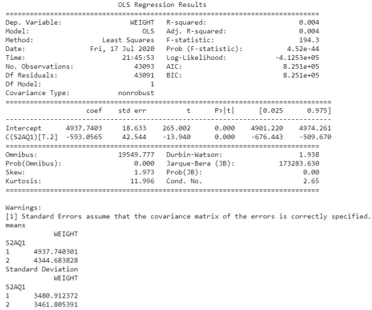
An Analysis of Variance(ANOVA) test revealed that from the NESARC codebook, the individuals who drank at least 1 alcoholic drink in life (2-level categorical explanatory variable) and Final Weight of individuals (quantitative response variable) were significantly associated, F=194.3, 1 df, p=4.52e-44 (where p-value is written in scientific notation).

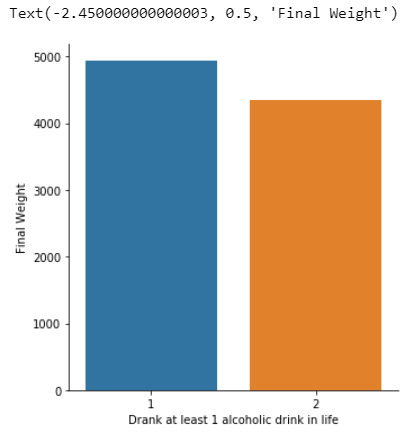
In the bivariate graph (C->Q) presented above, we can see the correlation between individuals who drank at least 1 alcoholic drink in life (explanatory variable) and Final Weight of individuals (response variable). Thus, it is explained in the above graph that individuals who drink alcohol gain more weight than those who don’t drink alcohol.

In the first place, for the moderating variable equal to 0, which is individuals who don’t have social phobia in last 12 months (sub2), a Analysis of Variance(ANOVA) test revealed that among the NESARC codebook, the individuals who drank at least 1 alcoholic drink in life (explanatory variable) and Final Weight of individuals (response variable) were significantly associated, F=200.6,1 df, p=1.99e-45 (where p-value is written in scientific notation). As a result, since the F-statistic value is very large and the p-value is significantly small, we can assume that there is a strong positive relationship between these two variables, when taking into account the subgroup of individuals who did not have social phobia in the last 12 months.

In the bivariate bar graph (C->Q) presented above, we can see the correlation between the individuals who drank at least 1 alcoholic drink in life (explanatory variable) and Final Weight of individuals (response variable), in the subgroup of individuals who did not have social phobia in the last 12 months(sub2). Obviously, it shows a positive relationship between these two variables, which means that the individuals who drank at least 1 alcoholic drink in life directly affects the Final weight of individuals, regarding the individuals who did not have social phobia in the last 12 months.

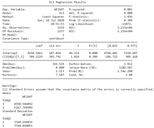
Secondly, for the moderating variable equal to 1, which is those  individuals who had social phobia in the last 12 months (sub3), an Analysis of Variance(ANOVA) test revealed that among NESARC codebook, the individuals who drank at least 1 alcoholic drink in life (explanatory variable) and Final Weight of individuals (response variable) were not significantly associated, F=1.036,1 df, p=0.309. As a result, since the F-statistic value is quite small and the p-value is significantly large, we can assume that there is no statistic relationship between these two variables, when taking into account the subgroup of individuals who had social phobia in the last 12 months.

In the bivariate bar graph (C->Q) presented above, we can see the correlation between individuals who drank at least 1 alcoholic drink in life (explanatory variable) and Final Weight of individuals (response variable), in the subgroup of individuals who had social phobia in the last 12 months (sub3). In fact, there is no positive relationship between these two variable, for those who had social phobia in the last 12 months.

SUMMARY:

It seems that both the direction and the size of the relationship between individuals who drank at least 1 alcoholic drink in life and Final Weight of individuals, is heavily affected by social phobia in the last 12 months. In other words, the individuals who had social phobia in the last 12 months, the correlation is considerably weak, whereas who did not have social phobia, the correlation is significantly strong and positive. Thus, the third variable moderates the association between individuals who drank at least 1 alcoholic drink in life and Final Weight of individuals.

[deepppp13]

Hypothesis Testing and Pearson’s Correlation

This assignment aims to statistically assess the evidence, provided by NESARC codebook, in favor of or against the association of number of Cigarettes smokers (Explanatory Variable) and both largest number of beers consumed and age on onset of first episode on Dysthymia (Response Variable). More specifically, since my research question includes only categorical variables, I selected three new quantitative variables from the NESARC codebook. Therefore, I redefined my hypothesis and examined the correlation between the age when the individuals started smoking everyday (S3AQ51) and both largest number of beers consumed on days when drank beer in last 12 months(S2AQ5E) and age on onset of first episode of Dysthymia(S4CQ5). As a result, in the first place, in order to visualize the association between Cigarettes smokers and both numbers of beers consumed on days when drank beer in last 12 months and age on onset of first episode of Dysthymia, I used seaborn library to produce a scatterplot for each response variables separately and interpreted the overall patterns, by describing the direction, as well as the form and the strength of the relationships. In addition, I ran Pearson correlation test (Q->Q) twice and measured the strength of the relationships between each pair of quantitative variables, by numerically generating both the correlation coefficients r and the associated p-values. For the code and the output I used Jupyter notebook (IDE).

The three quantitative variables that I used for my Pearson correlation test are:

PROGRAM:

import pandas as pd import numpy as np import seaborn import scipy.stats import matplotlib.pyplot as plt data = pd.read_csv('nesarc_pds.csv',low_memory=False) data1 = data.copy()

data['S3AQ41'] = pd.to_numeric(data['S3AQ41'],errors='coerce') data1['S3AQ41'] = pd.to_numeric(data1['S3AQ41'],errors='coerce') data['S2AQ5E'] = pd.to_numeric(data['S2AQ5E'],errors='coerce') data['S3AQ51'] = pd.to_numeric(data['S3AQ51'],errors='coerce') data1['S3AQ51'] = pd.to_numeric(data1['S3AQ51'],errors='coerce') data1['S4CQ5'] = pd.to_numeric(data1['S4CQ5'],errors='coerce')

subset1 = data[(data['S3AQ41']==1)] subsetc1 = subset1.copy() subset2 = data1[(data1['S3AQ41']==1)] subsetc2 = subset2.copy()

data['S2AQ5A'] = data['S2AQ5A'].replace(9,np.NaN) data['S2AQ5E'] = data['S2AQ5E'].replace(99,np.NaN) data['S3AQ51'] = data['S3AQ51'].replace(99,np.NaN) data1['S2AQ5A'] = data1['S2AQ5A'].replace(9,np.NaN) data1['S4CQ5'] = data1['S4CQ5'].replace(99,np.NaN) data1['S3AQ51'] = data1['S3AQ51'].replace(99,np.NaN)

data_clean1 = subset1.dropna() data_clean2 = subset2.dropna()

plt.figure(figsize=(16,8))   scat1 = seaborn.regplot(x="S3AQ51", y="S2AQ5E", fit_reg=True, data=subset1) plt.xlabel('Age when started smoking cigarettes everyday') plt.ylabel('Largest number of beers consumed on days when drank beer in last 12 months') plt.title('Scatterplot for the age when started smoking cigarettes everyday and the largest number of beers consumed on days when drank beer in last 12 months') plt.show() r1 = scipy.stats.pearsonr(data_clean1['S3AQ51'],data_clean1['S2AQ5E']) print(r1)

plt.figure(figsize=(16,6)) scat2 = seaborn.regplot(x="S3AQ51", y="S4CQ5", fit_reg=True, data=subset2) plt.xlabel('Age when started smoking cigarettes everyday') plt.ylabel('Age when experienced the first episode of Dysthymia') plt.title('Scatterplot for the age when started smoking cigaretes everyday and the age of the first episode of Dysthymia') plt.show() r2 = scipy.stats.pearsonr(data_clean2['S3AQ51'],data_clean2['S4CQ5']) print(r2)

OUTPUT:

The scatterplot presented above, illustrates the correlation between the age when started smoking cigarettes everyday (quantitative explanatory variable) and the largest number of beers consumed on days when drank beer in the last 12 months (quantitative response variable). The direction of the relationship is positive (increasing), which means that an increase in the age when started smoking cigarettes everyday is associated with an increase with the largest number of beers consumed on days when drank beer. In addition, since the points are scattered about a line, the relationship is linear. Regarding the strength of the relationship, from the pearson correlation test we can see that the correlation coefficient is equal to 0.11, which indicates a fairly weak linear relationship between the two quantitative variables. The associated p-value is equal to 9.40e-25 (p-value is written in scientific notation) and the fact that its very small means that the relationship is statistically significant. As a result, the association between the age when started smoking cigarettes everyday and the largest number of beers consumed on days when drank beer in the last 12 months is moderately weak, but it is highly unlikely that a relationship of this magnitude would be due to chance alone. Finally, by squaring the r, we can find the fraction of the variability of one variable that can be predicted by the other, which is fairly at 0.05.

For the association between the age when started smoking cigarettes everyday (quantitative explanatory variable) and the age when experienced the first episode of Dysthymia (quantitative response variable), the scatterplot presented above shows a positive linear relationship. Regarding the strength of the relationship, the pearson correlation test indicates that the correlation coefficient is equal to 0.17, which is interpreted to a weak linear relationship between the two quantitative variables. The associated p-values is equal to 4.54e-10 (p-value is written in scientific notation), which means that the relationship is statistically significant. Therefore, the association between the age when started smoking cigarettes everyday and the age when experienced the first episode on Dysthymia is weak, but it is highly unlikely that a relationship of this magnitude would be due to chance alone. Finally, by squaring the r, we can find the fraction of the variability of one variable that can be predicted by the other, which is very low at 0.05.

[deepppp13]

Hypothesis Testing and Chi Square Test of Independence

This assignment aims to directly test my hypothesis by evaluating, based on a sample of 4946 U.S. which resides in South region(REGION) aged between 25 to 40 years old(subsetc1), my research question with a goal of generalizing the results to the larger population of NESARC survey, from where the sample has been drawn. Therefore, I statistically assessed the evidence, provided by NESARC codebook, in favor of or against the association between Cigars smoked status and fear/avoidance of heights, in U.S. population in the South region. As a result, in the first place I used crosstab function, in order to produce a contingency table of observed counts and percentages for fear/avoidance of heights. Next, I wanted to examine if the Cigars smoked status (1= Yes or 2=no) variable ‘S3AQ42′, which is a 2-level categorical explanatory variable, is correlated with fear/avoidance of heights (’S8Q1A2′), which is a categorical response variable. Thus , I ran Chi-square Test of Independence(C->C) and calculated the  χ-squared values and the associated p-values for our specific conditions, so that null and alternate hypothesis are specified. In addition, in order visualize the association between frequency of cannabis use and depression diagnosis, I used catplot function to produce a bivariate graph. Furthermore, I used crosstab function once again and tested the association between the frequency of cannabis use (’S3BD5Q2E’), which is a 10-level categorical explanatory variable. In this case, for my second Test of Independence (C->C), after measuring the χ-square value and the p-value, in order to determine which frequency groups are different from the others, I performed a post hoc test, using Bonferroni Adjustment approach, since my explanatory variable has more than 2 levels. In this case of ten groups, I actually need to conduct 45 pair wise comparisons, but in fact I examined indicatively two and compared their p-values with the Bonferroni adjusted p-value, which is calculated by dividing p = 0.05 by 45. By this way it is possible to identify the situations where null hypothesis can be safely rejected without making an excessive type 1 error. For the code and the output I used Jupyter Notebook(IDE).

PROGRAM:

import pandas as pd

import numpy as np

import scipy.stats

import seaborn

import matplotlib.pyplot as plt

data = pd.read_csv('nesarc_pds.csv',low_memory=False)

data['AGE'] = pd.to_numeric(data['AGE'],errors='coerce')

data['REGION'] = pd.to_numeric(data['REGION'],errors='coerce')

data['S3AQ42'] = pd.to_numeric(data['S3AQ42'],errors='coerce')

data['S3BQ1A5'] = pd.to_numeric(data['S3BQ1A5'],errors='coerce')

data['S8Q1A2'] = pd.to_numeric(data['S8Q1A2'],errors='coerce')

data['S3BD5Q2E'] = pd.to_numeric(data['S3BD5Q2E'],errors='coerce')

data['MAJORDEP12'] = pd.to_numeric(data['MAJORDEP12'],errors='coerce')

subset1 = data[(data['AGE']>=25) & (data['AGE']<=40) & (data['REGION']==3)]

subsetc1 = subset1.copy()

subset2 = data[(data['AGE']>=18) & (data['AGE']<=30) & (data['S3BQ1A5']==1)]

subsetc2 = subset2.copy()

subsetc1['S3AQ42'] = subsetc1['S3AQ42'].replace(9,np.NaN)

subsetc1['S8Q1A2'] = subsetc1['S8Q1A2'].replace(9,np.NaN)

subsetc2['S3BD5Q2E'] = subsetc2['S3BD5Q2E'].replace(99,np.NaN)

cont1 = pd.crosstab(subsetc1['S8Q1A2'],subsetc1['S3AQ42'])

print(cont1)

colsum = cont1.sum()

contp = cont1/colsum

print(contp)

print ('Chi-square value, p value, expected counts, for fear/avoidance of heights within Cigar smoked status')

chsq1 = scipy.stats.chi2_contingency(cont1)

print(chsq1)

cont2 = pd.crosstab(subsetc2['MAJORDEP12'],subsetc2['S3BD5Q2E'])

print(cont2)

colsum = cont2.sum()

contp2 = cont2/colsum

print(contp2)

print('Chi-square value, p value, expected counts, for major depression within cannabis use status')

chsq2 = scipy.stats.chi2_contingency(cont2)

print(chsq2)

recode = {1:10,2:9,3:8,4:7,5:6,6:5,7:4,8:3,9:2,10:1}

subsetc2['CUFREQ'] = subsetc2['S3BD5Q2E'].map(recode)

subsetc2['CUFREQ'] = subsetc2['CUFREQ'].astype('category')

subsetc2['CUFREQ'] = subsetc2['CUFREQ'].cat.rename_categories(['Once a year','2 times a year','3 to 6 times a year','7 to 11 times a year','Once a month','2 to 3 times a month','1 to 2 times a week','3 to 4 times a week','Nearly Everyday','Everyday'])

plt.figure(figsize=(16,8))

ax1 = seaborn.catplot(x='CUFREQ',y='MAJORDEP12', data=subsetc2, kind="bar", ci=None)

ax1.set_xticklabels(rotation=40, ha="right")

plt.xlabel('Frequency of cannabis use')

plt.ylabel('Proportion of Major Depression')

plt.show()

recode={1:1,9:9}

subsetc2['COMP1v9'] = subsetc2['S3BD5Q2E'].map(recode)

cont3 = pd.crosstab(subsetc2['MAJORDEP12'],subsetc2['COMP1v9'])

print(cont3)

colsum = cont3.sum()

contp3 = cont3/colsum

print(contp3)

print('Chi-square value, p value, expected counts, for major depression within pair comparisons of frequency groups -Everyday- and -2 times a year-')

chsq3 = scipy.stats.chi2_contingency(cont3)

print(chsq3)

recode={4:4,9:9}

subsetc2['COMP4v9'] = subsetc2['S3BD5Q2E'].map(recode)

cont4 = pd.crosstab(subsetc2['MAJORDEP12'],subsetc2['COMP4v9'])

print(cont4)

colsum = cont4.sum()

contp4 = cont4/colsum

print(contp4)

print('Chi-square value, p value, expected counts, for major depression within pair comparisons of frequency groups -1 to 2 times a week- and -2 times a year-')

chsq4 = scipy.stats.chi2_contingency(cont4)

print(chsq4)

*******************************************************************************************

OUTPUT: 

When examining the patterns of association between fear/avoidance of heights (categorical response variable) and Cigars use status (categorical explanatory variable), a chi-square test of independence revealed that among aged between 25 to 40 in the South region(subsetc1), those who were Cigars users, were more likely to have the fear/avoidance of heights(26%), compared to the non-users(20%), X2=0.26,1 df, p=0.6096. As a result, since our p-value is not smaller than 0.05(Level of Significance), the data does not provide enough evidence against the null hypothesis. Thus, we accept the null hypothesis , which indicates that there is no positive correlation between Cigar users and fear/avoidance of heights.

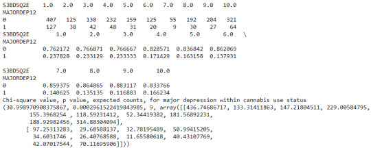
A Chi Square test of independence revealed that among cannabis users aged between 18 to 30 years old (susbetc2), the frequency of cannabis use (explanatory variable collapsed into 10 ordered categories) and past year depression diagnosis (response binary categorical variable) were significantly associated, X2 = 30.99,9 df, p=0.00029.

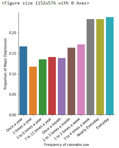
In the bivariate graph(C->C) presented above, we can see the correlation between frequency of cannabis use (explanatory variable) and major depression diagnosis in the past year (response variable). Obviously, we have a left-skewed distribution, which indicates that the more an individual (18-30) smoked cannabis, the better were the cases to have experienced depression in the last 12 months.

The post hoc comparison (Bonferroni Adjustment) of rates of major depression by the pair of “Every day” and “2 times a year” frequency categories, revealed that the p-value is 0.00019 and the percentages of major depression diagnosis for each frequency group are 23.7% and 11.6% respectively. As a result, since the p-value is smaller than the Bonferroni adjusted p-value (adj p-value = 0.05 / 45 = 0.0011>0.00019), we can assume that these two rates are significantly different from one another. Therefore, we reject the null hypothesis and accept the alternate. 

Similarly, the post hoc comparison (Bonferroni Adjustment) of rates of major depression by the pair of "1 or 2 times a week” and “2 times a year” frequency categories, indicated that the p-value is 0.107 and the proportions of major depression diagnosis for each frequency group are 17.1% and 11.6% respectively. As a result, since the p-value is larger than the Bonferroni adjusted p-value (adj p-value = 0.05 / 45 = 0.107>0.0011), we can assume that these two rates are not significantly different from one another. Therefore, we accept the null hypothesis.

[deepppp13]

ANOVA

This assignment aims to directly test my hypothesis by evaluating, based on a sample of 2051 U.S. candidates who drink when they are not with family(H1TO13) and are White(H1GI6A) OR American Indian or Native American(H1GI6B) in race(subset1), my research question with the goal of generalizing the results to the larger population of ADDHEALTH survey, from where the sample has been drawn. Therefore, I statistically assessed the evidence, provided by  ADDHEALTH codebook, in favor of or against the association between Drinkers and Special Romantic Relationship, in U.S. population. As a result, in the first place I used the OLS function in order to examine if Special Romantic Relationship in the past 18 months(H1RR1), which is a categorical explanatory variables, is correlated with the quantity of drinks an individual had each time during the past 12 months(H1TO16), which is a quantitative response variable. Thus, I ran ANOVA (Analysis of Variable) method (C- >Q) once and calculated the F-statistics and the associated p-values, so that null and alternate hypothsis are specified. Furthermore, I used OLS function once again and tested the association between frequency of drinks had during the past 12 months(H1TO15),which is a 6-level categorical explanatory variable, and the quantity of drinks a particular had each time during the past 12 months(H1TO15),which is a quantitative response variable. In this case, for my second one-way ANOVA(C- >Q),after measuring the F-statistic and the p-value, I used Tukey HSDT to perform a post hoc test, that conducts post hoc paired comparisons in the context of my ANOVA, since my explanatory variable has more than 2 levels. By this way it is possible to identify the situations where null hypothesis can be safely rejected without making an excessive type 1 error. In addition, both means and standard deviations of quantity response variable, were measured separately in each ANOVA, grouped by the explanatory response variables using the groupby function. For the code and the output I used Jupyter Notebook (IDE).

PROGRAM:

import pandas as pd

import numpy as np

import statsmodels.formula.api as smf

import statsmodels.stats.multicomp as multi

df = pd.read_csv('addhealth_pds.csv',low_memory=False)

subset1 = df[(df['H1TO13']==1) & (df['H1GI6A']==1) | (df['H1GI6C']==1)]

subset1['H1TO16'] = subset['H1TO16'].replace([96,97,98,99],np.NaN)

subset1['H1RR1'] = subset['H1RR1'].replace([6,8,9],np.NaN)

subset1['H1GI6A'] = subset['H1GI6A'].replace([6,8],np.NaN)

subset1['H1GI6C'] = subset['H1GI6C'].replace([6,8],np.NaN)

subset1['H1TO13'] = subset['H1TO13'].replace([7,8],np.NaN)

sub1 = subset1[['H1TO16','H1RR1']].dropna()

model1 = smf.ols(formula='H1TO16 ~ C(H1RR1)',data=sub1)

res1 = model1.fit()

print(res1.summary())

print('Means for drink quantity for past 12 months by special romantic relationship status')

m1 = sub1.groupby('H1RR1').mean()

print(m1)

print('Standard Deviation for drink quantity for past 12 months by special romantic relationship status')

s1 = sub1.groupby('H1RR1').std()

print(s1)

subset1['H1TO15'] = subset1['H1TO15'].replace([7,96,97,98],np.NaN)

sub2 = subset1[['H1TO16','H1TO15']].dropna()

model2 = smf.ols(formula='H1TO16 ~ C(H1TO15)',data=sub2).fit()

print(model2.summary())

print("Means for drinking quantity by frequency of drinks on days status")

m2 = sub2.groupby('H1TO15').mean()

print(m2)

print("Standard deviation for drinking quantity by frequency of drinks on days status")

s2 = sub2.groupby('H1TO15').std()

print(s2)

mc1=multi.MultiComparison(sub2['H1TO16'],sub2['H1TO15']).tukeyhsd()

print(mc1.summary())

OUTPUT :

When examining the association between the number of drinks had each time (quantitative response variable) and Special Romantic Relationship (categorical explanatory variable), an Analysis of Variance(ANOVA) revealed that drinkers when not with family and are American Indian or Native America in race(subset1), those with Special Romantic Relationship reported drinking marginally equal quantity of drinks each time (Mean=6.34,s.d.  ±7.33) compared to those without Special Romantic Relationship(Mean=5.67,  ±6.35) , F(1,1779)=3.016, p=0.0862>0.05. As a result, since our p-value is significantly large, in this case the data is not considered to be surprising enough when the null hypothesis is true. Consequently, there are not enough evidence to reject the null hypothesis and accept the alternate, thus there is no positive association between Special Romantic Relationship and quantity of drinks had each time.

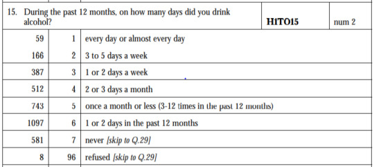
ANOVA revealed that among U.S. population who drink when they are not with family(H1TO13) and are White(H1GI6A) OR American Indian or Native American(H1GI6B) in race(subset1), frequency of drinks on days(collapsed into 6 ordered categories, which is the categorical explanatory variable) and quantity of drinks had each time per day (quantitative response variable) were relatively associated, F(5,1777)=27.63, p=5.09e-27<0.05 (p value is written in scientific notation). Post hoc comparisons of mean number of drinks each time by pairs of drinks frequency categories, revealed that those individuals drinking every day (or 3 to 5 days a week) reported drinking significantly more on average daily (every day: Mean=10.27, s.d.  ±9.47, 3 to 5 days a week: Mean=8.26, s.d.  ±5.57)  compared to those drinking 2 or 3 days a month (Mean=7.29, s.d.  ±8.16), or less. As a result, there are some pair cases in which frequency and drinking quantity of drinkers, are positive correlated.

In order to conduct post hoc paired comparisons in the context of my ANOVA, examining the association between frequency of drinks and number of drinks had each time, I used the Tukey HSD test. The table presented above, illustrates the differences in drinking quantity for each frequency of drinks use frequency group and help us identify the comparisons in which we can reject the null hypothesis and accept the alternate hypothesis, that is, in which reject equals true. In cases where reject equals false, rejecting the null hypothesis resulting in inflating a type 1 error.