engrflores - Tumblr blog

engrflores · 4 years ago

Text

Machine learning for Data Analysis

Machine learning for Data Analysis - Week 4 ( Running a k-means Cluster Analysis )

This is the last assignment for the Machine learning for data analysis course, fourth from a series of five courses from Data Analysis and Interpretation administered by Wesleyan University. In this assignment, we have to run a K-means Cluster Analysis.

A k-means cluster analysis was conducted to identify underlying subgroups based on their similarity of responses on 7 variables that represent characteristics that could have an impact on Personal Income. Clustering variables included three binary variables Gender (0=Female,1=Male), Major depression (0=No,1=Yes) and Present situation includes Working Full Time (0=No, 1=Yes), as well as other categorical variables Educational attainment, Self-perceived current health, How often drank liquor and Marital status. All clustering variables were standardized to have a mean of 0 and a standard deviation of 1.

Data were randomly split into a training set that included 70% of the observations and a test set that included 30% of the observations. A series of k-means cluster analyses were conducted on the training data specifying k=1-9 clusters, using Euclidean distance. The variance in the clustering variables that was accounted for by the clusters (r-square) was plotted for each of the nine cluster solutions in an elbow curve to provide guidance for choosing the number of clusters to interpret.

Running a k-means Cluster Analysis

The first thing to do is to import the libraries and prepare the data to be used. To run the k-means Cluster Analysis we must standardize the predictors to have mean = 0 and standard deviation = 1. After that, we make 9 analysis with the data, the first one with one cluster increasing a cluster per experiment.

Selecting K with the Elbow Method

In our case, the bend in the elbow appears to be at two clusters and at three clusters.

To help us figure out which of the solutions is best, we are going to use the canonical discriminate analysis.

First, let’s see the results with three clusters:

We can see that these three clusters here are well separated, but the observations are more spread out indicating less correlation among the observations and higher within cluster variance. This suggests that the four cluster solution might be better. So, let’s see the results with four clusters.

The three clusters plot show us that there is little or no overlap between the clusters, they are well separated and the observations are less spread out indicating higher correlation among the observations and less within cluster variance.

After that, we begin the multiple steps to merge cluster assignment with clustering variables to examine cluster variable means by cluster.

On the first cluster, which is cluster 0, these individuals are likely to be male, likelihood of not in a current relationship, more prone to depression, lower educational attainment, poor self-perception of current health status, likelihood of always getting drunk and not working full time.

On the second cluster, which is cluster 1, these individuals are likely to be male, likelihood of not in a current relationship, lowest likelihood on depression, highest likelihood of having high educational attainment, highest likelihood of having positive self-perception of current health status, likelihood of getting drunk and with highest likelihood of working full time.

On the third cluster, which is cluster 2, these individuals are likely to be female, likelihood of being in a current relationship, less prone to depression, likelihood of having high educational attainment, likelihood of having positive self-perception of current health status, lowest likelihood of getting drunk and with likelihood of working full time.

We'll use analysis of variance to test whether there are significant differences between clusters on the categorical Income variable.

Here are the results. The analysis of variance summary table indicates that the clusters differed significantly on Income.

Finally, let's see how the clusters differ on Income.

When we examine the means, we find that not surprisingly, individuals in cluster 1, are the highest income group, and adolescents in cluster 0, are the lowest income group.

The tukey test shows that the clusters 0 and 1 differed significantly in mean INCOME, although 0 and 2 & 1 & 2 don’t differ significantly, their mean difference is small.

My Python program:

from pandas import Series, DataFrame import pandas as pd import numpy as np import matplotlib.pylab as plt from sklearn.model_selection import train_test_split from sklearn import preprocessing from sklearn.cluster import KMeans

# bug fix for display formats to avoid run time errors pd.set_option('display.float_format', lambda x:'%.2f'%x)

#Load the dataset data = pd.read_csv("NESARC_Data_Set.csv", low_memory=False)

# DATA MANAGEMENT # convert values to numeric data['MAJORDEPLIFE'] = pd.to_numeric(data['MAJORDEPLIFE'], errors='coerce') data['S1Q10A'] =pd.to_numeric(data['S1Q10A'], errors='coerce') data['GENDER']=pd.to_numeric(data['SEX'],errors='coerce') data['EDUC']=pd.to_numeric(data['S1Q6A'],errors='coerce') data['CHEALTH']=pd.to_numeric(data['S1Q16'],errors='coerce') data['DRANKLIQ']=pd.to_numeric(data['S2AQ7B'],errors='coerce') data['MARITAL']=pd.to_numeric(data['MARITAL'],errors='coerce') data['WORKFULL']=pd.to_numeric(data['S1Q7A1'],errors='coerce')

# subset data to age 18-35 sub1 = data[(data['AGE'] >= 18) & (data['AGE'] <= 65) & (data['S1Q10A'] >= 0) & (data['S1Q10A'] <= 100000)] B1=sub1.copy()

def INCOME (row): if row['S1Q10A']<=23000: return 0 elif row['S1Q10A']<=100000: return 1 B1['INCOME'] = B1.apply (lambda row: INCOME (row),axis=1)

# recode explanatory variables recode2 = {1:1,2:0} B1['GENDER'] = data['SEX'].map(recode2) B1['WORKFULL'] = data['WORKFULL'].map(recode2) recode3 = {1:4,2:3,3:2,4:1,5:0} B1['CHEALTH'] = data['CHEALTH'].map(recode3) recode4 = {10:0,9:1,8:2,7:3,6:4,5:5,4:6,3:7,2:8,1:9} B1['DRANKLIQ'] = data['DRANKLIQ'].map(recode4)

# convert INCOME to numerical B1['INCOME'] =pd.to_numeric(B1['INCOME'], errors='coerce') B1['GENDER'] =pd.to_numeric(B1['GENDER'], errors='coerce') #B1['DYSLIFE'] =pd.to_numeric(data['DYSLIFE'], errors='coerce') B1['EDUC'] =pd.to_numeric(data['EDUC'], errors='coerce') B1['DRANKLIQ'] =pd.to_numeric(B1['DRANKLIQ'], errors='coerce') B1['MARITAL'] =pd.to_numeric(data['MARITAL'], errors='coerce') B1['WORKFULL']=pd.to_numeric(B1['WORKFULL'],errors='coerce')

data_clean = B1.dropna()

# subset clustering variables cluster=data_clean[['MAJORDEPLIFE','GENDER','EDUC','CHEALTH','MARITAL','DRANKLIQ','WORKFULL']]

# standardize clustering variables to have mean=0 and sd=1 clustervar=cluster.copy() from sklearn import preprocessing clustervar['MAJORDEPLIFE']=preprocessing.scale(clustervar['MAJORDEPLIFE'].astype('float64')) clustervar['GENDER']=preprocessing.scale(clustervar['GENDER'].astype('float64')) clustervar['EDUC']=preprocessing.scale(clustervar['EDUC'].astype('float64')) clustervar['CHEALTH']=preprocessing.scale(clustervar['CHEALTH'].astype('float64')) clustervar['DRANKLIQ']=preprocessing.scale(clustervar['DRANKLIQ'].astype('float64')) clustervar['MARITAL']=preprocessing.scale(clustervar['MARITAL'].astype('float64')) clustervar['WORKFULL']=preprocessing.scale(clustervar['WORKFULL'].astype('float64'))

# split data into train and test sets clus_train, clus_test = train_test_split(clustervar, test_size=.3, random_state=123)

# k-means cluster analysis for 1-9 clusters from scipy.spatial.distance import cdist clusters=range(1,10) meandist=[]

for k in clusters: model=KMeans(n_clusters=k) model.fit(clus_train) clusassign=model.predict(clus_train) meandist.append(sum(np.min(cdist(clus_train, model.cluster_centers_, 'euclidean'), axis=1)) / clus_train.shape[0])

""" Plot average distance from observations from the cluster centroid to use the Elbow Method to identify number of clusters to choose """

plt.plot(clusters, meandist) plt.xlabel('Number of clusters') plt.ylabel('Average distance') plt.title('Selecting k with the Elbow Method') plt.show()

# Interpret 3 cluster solution model3=KMeans(n_clusters=3) model3.fit(clus_train) clusassign=model3.predict(clus_train) # plot clusters

from sklearn.decomposition import PCA pca_2 = PCA(2) plot_columns = pca_2.fit_transform(clus_train) plt.scatter(x=plot_columns[:,0], y=plot_columns[:,1], c=model3.labels_,) plt.xlabel('Canonical variable 1') plt.ylabel('Canonical variable 2') plt.title('Scatterplot of Canonical Variables for 3 Clusters') plt.show()

""" BEGIN multiple steps to merge cluster assignment with clustering variables to examine cluster variable means by cluster """ # create a unique identifier variable from the index for the # cluster training data to merge with the cluster assignment variable clus_train.reset_index(level=0, inplace=True) # create a list that has the new index variable cluslist=list(clus_train['index']) # create a list of cluster assignments labels=list(model3.labels_) # combine index variable list with cluster assignment list into a dictionary newlist=dict(zip(cluslist, labels)) newlist # convert newlist dictionary to a dataframe newclus=DataFrame.from_dict(newlist, orient='index') newclus # rename the cluster assignment column newclus.columns = ['cluster']

# now do the same for the cluster assignment variable # create a unique identifier variable from the index for the # cluster assignment dataframe # to merge with cluster training data newclus.reset_index(level=0, inplace=True) # merge the cluster assignment dataframe with the cluster training variable dataframe # by the index variable merged_train=pd.merge(clus_train, newclus, on='index') merged_train.head(n=100) # cluster frequencies merged_train.cluster.value_counts()

""" END multiple steps to merge cluster assignment with clustering variables to examine cluster variable means by cluster """

# FINALLY calculate clustering variable means by cluster clustergrp = merged_train.groupby('cluster').mean() print ("Clustering variable means by cluster") print(clustergrp)

# validate clusters in training data by examining cluster differences in GPA using ANOVA # first have to merge GPA with clustering variables and cluster assignment data gpa_data=data_clean['INCOME'] # split GPA data into train and test sets gpa_train, gpa_test = train_test_split(gpa_data, test_size=.3, random_state=123) gpa_train1=pd.DataFrame(gpa_train) gpa_train1.reset_index(level=0, inplace=True) merged_train_all=pd.merge(gpa_train1, merged_train, on='index') sub1 = merged_train_all[['INCOME', 'cluster']].dropna()

import statsmodels.formula.api as smf import statsmodels.stats.multicomp as multi

gpamod = smf.ols(formula='INCOME ~ C(cluster)', data=sub1).fit() print (gpamod.summary())

print ('means for INCOME by cluster') m1= sub1.groupby('cluster').mean() print (m1)

print ('standard deviations for INCOME by cluster') m2= sub1.groupby('cluster').std() print (m2)

mc1 = multi.MultiComparison(sub1['INCOME'], sub1['cluster']) res1 = mc1.tukeyhsd() print(res1.summary())

0 notes

engrflores · 4 years ago

Text

Machine learning for Data Analysis

Machine learning for Data Analysis - Week 3 ( Running a Lasso Regression Analysis )

This is the third assignment for the Machine learning for data analysis course, fourth from a series of five courses from Data Analysis and Interpretation administered by Wesleyan University. In this assignment, we have to run a Random Forest.

This week’s assignment involves running a lasso regression analysis. Lasso regression analysis is a shrinkage and variable selection method for linear regression models. The goal of lasso regression is to obtain the subset of predictors that minimizes prediction error for a quantitative response variable. The lasso does this by imposing a constraint on the model parameters that causes regression coefficients for some variables to shrink toward zero. Variables with a regression coefficient equal to zero after the shrinkage process are excluded from the model. Variables with non-zero regression coefficients variables are most strongly associated with the response variable. Explanatory variables can be either quantitative, categorical or both.

My binary response or target variable is Personal Income (0=Low Income (<=$23000), 1=High Income (<=$100000)) and my Explanatory or predictor variable are Major depression (0=NO,1=YES), Gender (0=Female, 1=Male) and Dysthymia (0=NO, 1=YES).

Here are the results:

The results show that of my 3 predictor variables, only 1 variable was selected in the final model. We standardized the values of our variables to be on the same scale. So, we can also use the size of the regression coefficients to tell us which predictors are the strongest predictors of school connectedness.

Gender is most strongly and negatively associated with Income.

Plot of Regression Coefficients Progression for Lasso Paths

This plot shows the relative importance of the predictor selected at any step of the selection process, how the regression coefficients changed with the addition of a new predictor at each step, as well as the steps at which each variable entered the model. As we already know from looking at the list of the regression coefficients Gender, the orange line, had the decreasing regression coefficients as penalty parameter increases. Also, both Major depression and Dysthymia remains at a value of zero coefficient as penalty parameter increases. This can be seen from the results above that their regression coefficients have been shrink toward zero and therefore excluded from the model. We cannot Identify which variable was first entered into the model first and which is second because their least values of penalty parameters are very close based on the plot.

Plot Of Mean Squared Error On Each Fold

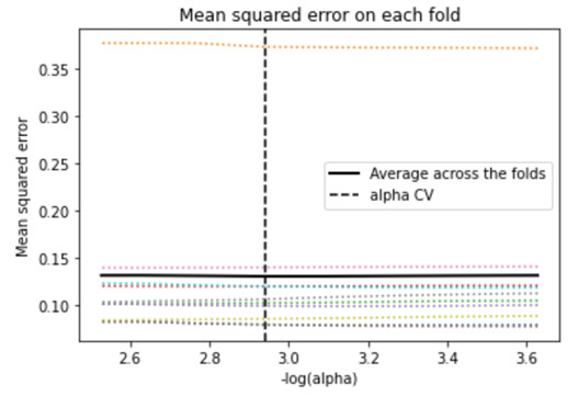
We can see that there is variability across the individual cross-validation folds in the training data set, but the change in the mean square error as variables are added to the model follows the same pattern for each fold. It follows a straight line at each fold which means that it has constant Mean squared error across each fold. Adding more predictors doesn't lead to much reduction in the mean square error.

Mean Squared Error from Training and Test Data

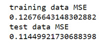
As expected, the selected model was less accurate in predicting Income in the test data, but the test mean square error was pretty close to the training mean square error. This suggests that prediction accuracy was pretty stable across the two data sets.

R-Square from Training and Test Data

The R-square values were 0.01257nd 0.0278, indicating that the selected model explained 1.257% and 2.78% of the variance in Income for the training and test sets, respectively. The Gender variable is accounted for 1.257% of the variance in the school connectedness response variable.

Data were randomly split into a training set that included 70% of the observations and a test set that included 30% of the observations. The least angle regression algorithm with k=10 fold cross validation was used to estimate the lasso regression model in the training set, and the model was validated using the test set. The change in the cross validation average (mean) squared error at each step was used to identify the best subset of predictor variables.

Two variables were removed in my model which is Major depression and Dysthymia out of my 3 predictor variables.

My Python Program:

import pandas as pd import numpy as np import matplotlib.pylab as plt from sklearn.model_selection import train_test_split from sklearn.linear_model import LassoLarsCV

# bug fix for display formats to avoid run time errors pd.set_option('display.float_format', lambda x:'%.2f'%x)

#Load the dataset data = pd.read_csv("NESARC_Data_Set.csv", low_memory=False)

# subset data to age 18-35 sub1 = data[(data['AGE'] >= 18) & (data['AGE'] <= 35) & (data['S1Q10A'] >= 0) & (data['S1Q10A'] <= 100000)] B1=sub1.copy()

def INCOME (row): if row['S1Q10A']<=23000: return 0 elif row['S1Q10A']<=100000: return 1 B1['INCOME'] = B1.apply (lambda row: INCOME (row),axis=1)

# recode explanatory variables to include 0 recode2 = {1:1,2:0} B1['GENDER'] = B1['SEX'].map(recode2)

# convert INCOME to numerical B1['INCOME'] =pd.to_numeric(B1['INCOME'], errors='coerce') B1['GENDER'] =pd.to_numeric(data['GENDER'], errors='coerce') B1['DYSLIFE'] =pd.to_numeric(data['DYSLIFE'], errors='coerce') B1['MAJORDEPLIFE'] =pd.to_numeric(data['MAJORDEPLIFE'], errors='coerce')

data_clean = B1.dropna()

#select predictor variables and target variable as separate data sets predvar= data_clean[['MAJORDEPLIFE','GENDER','DYSLIFE']]

target = data_clean.INCOME

# standardize predictors to have mean=0 and sd=1 predictors=predvar.copy() from sklearn import preprocessing predictors['MAJORDEPLIFE']=preprocessing.scale(predictors['MAJORDEPLIFE'].astype('float64')) predictors['GENDER']=preprocessing.scale(predictors['GENDER'].astype('float64')) predictors['DYSLIFE']=preprocessing.scale(predictors['DYSLIFE'].astype('float64'))

# split data into train and test sets pred_train, pred_test, tar_train, tar_test = train_test_split(predictors, target, test_size=.3, random_state=123)

# specify the lasso regression model model=LassoLarsCV(cv=10, precompute=False).fit(pred_train,tar_train)

# print variable names and regression coefficients dict(zip(predictors.columns, model.coef_))

# plot coefficient progression m_log_alphas = -np.log10(model.alphas_) ax = plt.gca() plt.plot(m_log_alphas, model.coef_path_.T) plt.axvline(-np.log10(model.alpha_), linestyle='--', color='k', label='alpha CV') plt.ylabel('Regression Coefficients') plt.xlabel('-log(alpha)') plt.title('Regression Coefficients Progression for Lasso Paths')

# plot mean square error for each fold m_log_alphascv = -np.log10(model.cv_alphas_) plt.figure() plt.plot(m_log_alphascv, model.mse_path_, ':') plt.plot(m_log_alphascv, model.mse_path_.mean(axis=-1), 'k', label='Average across the folds', linewidth=2) plt.axvline(-np.log10(model.alpha_), linestyle='--', color='k', label='alpha CV') plt.legend() plt.xlabel('-log(alpha)') plt.ylabel('Mean squared error') plt.title('Mean squared error on each fold')

# MSE from training and test data from sklearn.metrics import mean_squared_error train_error = mean_squared_error(tar_train, model.predict(pred_train)) test_error = mean_squared_error(tar_test, model.predict(pred_test)) print ('training data MSE') print(train_error) print ('test data MSE') print(test_error)

# R-square from training and test data rsquared_train=model.score(pred_train,tar_train) rsquared_test=model.score(pred_test,tar_test) print ('training data R-square') print(rsquared_train) print ('test data R-square') print(rsquared_test) # plot mean square error for each fold m_log_alphascv = -np.log10(model.cv_alphas_) plt.figure() plt.plot(m_log_alphascv, model.mse_path_, ':') plt.plot(m_log_alphascv, model.mse_path_.mean(axis=-1), 'k', label='Average across the folds', linewidth=2) plt.axvline(-np.log10(model.alpha_), linestyle='--', color='k', label='alpha CV') plt.legend() plt.xlabel('-log(alpha)') plt.ylabel('Mean squared error') plt.title('Mean squared error on each fold')

0 notes

engrflores · 4 years ago

Text

Machine learning for Data Analysis

Machine learning for Data Analysis - Week 2 ( Running a Random Forest )

This is the second assignment for the machine learning for data analysis course, fourth from a series of five courses from Data Analysis and Interpretation ministered from Wesleyan University. In this assignment, we have to run a Random Forest.

My binary response or target variable is Personal Income (0=Low Income (<=$23000), 1=High Income (<=$100000)) and my Explanatory or predictor variables are Major depression (0=NO,1=YES), Gender (0=Female, 1=Male) and Dysthymia (0=NO, 1=YES).

pred_train.shape

pred_test.shape

tar_train.shape

tar_test.shape

The training sample has 306 observations or rows, 60% of our original sample, and 3 explanatory variables. The test sample has 205 observations or rows, 40% of the original sample. And again 3 explanatory variables or columns.

Confusion Matrix

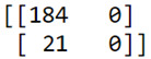
The diagonal, 184 and 0, represent the number of true negative for personal smoking, and the number of true positives, respectively. The 21, on the bottom left, represents the number of false negatives. Classifying high income as low income. And the 0 on the top right, the number of false positives, classifying low income as a high income which is none in our case.

In my confusion matrix, the training data statistical model incorrectly classified a total of 21 of the 205 observations in the test sample, meaning that the statistical model misclassified 10% of the observations in the test data set.

21 + 0 = 21 incorrectly classified

Test error rate = % misclassified = 21/205 = 10%

Accuracy Score:

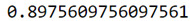
which is approximately 0.8976, which suggests that the decision tree model has classified 89.76% of the sample correctly as either regular or not regular smokers.

Given that we don't interpret individual trees in a random forest, the most helpful information to be gotten from a forest is arguably the measured importance for each explanatory variable. Also called the features. Based on how many votes or splits each has produced in the 25 tree ensemble.

Accuracy score vs Number of trees

As we can see, all the trees has the same accuracy of about 89%.

Feature Important scores

The variables are listed in the order they've been named earlier in the code. Starting with Major depression, Gender, and ending with Dysthymia. As we can see the variables with the highest important score at 0.499 is Gender and the variable with the lowest important score is Asian Dysthymia at 0.08.

My Python program:

from pandas import Series, DataFrame import pandas as pd import numpy as np import matplotlib.pylab as plt import statistics from sklearn.model_selection import train_test_split from sklearn.tree import DecisionTreeClassifier from sklearn.metrics import classification_report import sklearn.metrics # Feature Importance from sklearn import datasets from sklearn.ensemble import ExtraTreesClassifier

# bug fix for display formats to avoid run time errors pd.set_option('display.float_format', lambda x:'%.2f'%x)

#Load the dataset

data = pd.read_csv("NESARC_Data_Set.csv", low_memory=False)

# convert values to numeric data['MAJORDEPLIFE'] = pd.to_numeric(data['MAJORDEPLIFE'], errors='coerce') data['S1Q10A'] =pd.to_numeric(data['S1Q10A'], errors='coerce') data['GENDER']=pd.to_numeric(data['SEX'],errors='coerce') data['DYSLIFE']=pd.to_numeric(data['DYSLIFE'],errors='coerce')

# subset data to age 18-35 sub1 = data[(data['AGE'] >= 18) & (data['AGE'] <= 35) & (data['S1Q10A'] >= 0) & (data['S1Q10A'] <= 100000)] B1=sub1.copy()

def INCOME (row): if row['S1Q10A']<=23000: return 0 elif row['S1Q10A']<=100000: return 1 B1['INCOME'] = B1.apply (lambda row: INCOME (row),axis=1)

# recode explanatory variables to include 0 recode2 = {1:1,2:0} B1['GENDER'] = B1['SEX'].map(recode2)

data_clean = B1.dropna()

""" Modeling and Prediction """ #Split into training and testing sets

predictors = data_clean[['MAJORDEPLIFE','GENDER','DYSLIFE']]

targets = data_clean.INCOME

#Train = 60%, Test = 40% pred_train, pred_test, tar_train, tar_test = train_test_split(predictors, targets, test_size=.4)

print(pred_train.shape) print(pred_test.shape) print(tar_train.shape) print(tar_test.shape)

#Build model on training data from sklearn.ensemble import RandomForestClassifier

classifier=RandomForestClassifier(n_estimators=25) classifier=classifier.fit(pred_train,tar_train)

predictions=classifier.predict(pred_test)

print(sklearn.metrics.confusion_matrix(tar_test,predictions)) print(sklearn.metrics.accuracy_score(tar_test, predictions))

# fit an Extra Trees model to the data model = ExtraTreesClassifier() model.fit(pred_train,tar_train) # display the relative importance of each attribute print(model.feature_importances_)

""" Running a different number of trees and see the effect of that on the accuracy of the prediction """

trees=range(25) accuracy=np.zeros(25)

for idx in range(len(trees)): classifier=RandomForestClassifier(n_estimators=idx + 1) classifier=classifier.fit(pred_train,tar_train) predictions=classifier.predict(pred_test) accuracy[idx]=sklearn.metrics.accuracy_score(tar_test, predictions)

plt.cla() plt.plot(trees, accuracy)

print(accuracy) print(statistics.mean(accuracy))

0 notes

engrflores · 4 years ago

Text

Machine learning for Data Analysis

Machine learning for Data Analysis - Week 1 ( Running a Classification Tree )

This is the first assignment for the machine learning for data analysis course, fourth from a series of five courses from Data Analysis and Interpretation ministered from Wesleyan University. In this assignment, we have to run a classification tree.

This week’s assignment involves decision trees, and more specifically, classification trees. Decision trees are predictive models that allow for a data driven exploration of nonlinear relationships and interactions among many explanatory variables in predicting a response or target variable. When the response variable is categorical (two levels), the model is a called a classification tree. Explanatory variables can be either quantitative, categorical or both. Decision trees create segmentations or subgroups in the data, by applying a series of simple rules or criteria over and over again which choose variable constellations that best predict the response (i.e. target) variable.

My binary response or target variable is Personal Income (0=Low Income (<=$23000), 1=High Income (<=$100000)) and my binary Explanatory or predictor variables are Major depression (0=NO,1=YES) and Gender (0=Female, 1=Male).

Running a Classification Tree

Here I show a tree, my binary Income variable, as the target. And both major depression and gender as the predictor or explanatory variables.

The resulting tree starts with the split on X[1], our second explanatory variable, Gender. If the value for Gender is less than 0.5, that is Female since my binary variable has values of zero equal no and one equal yes.

On the left side of the split, it includes 168 Females of the 306 individuals in my training sample. From this node, another split is made on major depression on the left side, variable X[0], such that among those individuals who are Female in the first split and also has major depression in the second split, 84 of them are low income young adults, while only 33 are high income young adults. While on the right side of the split, Female young adults without major depression, 66 of them are high income and only 7 are low income young adults.

On the right side of the split, it includes 138 Males of the 306 individuals in my training sample. From this node, another split is made on major depression on the left side, variable X[0], such that among those individuals who are Male in the first split and also has major depression in the second split, 68 of them are low income young adults, while only 21 are high income young adults. While on the right side of the split, Male young adults without major depression, 40 of them are high income and only 9 are low income young adults.

Here I request the shape of these predictor and target training and test samples:

pred_train.shape

pred_test.shape

tar_train.shape

tar_test.shape

The training sample has 306 observations or rows, 60% of our original sample, and 2 explanatory variables. The test sample has 205 observations or rows, 40% of the original sample. And again 2 explanatory variables or columns.

Next, we predict for the test values and then call in the confusion matrix function which we passed the target test sample:

This shows the correct and incorrect classifications of our decision tree. The diagonal, 178 and 0, represent the number of true negative for personal smoking, and the number of true positives, respectively. The 27, on the bottom left, represents the number of false negatives. Classifying high income as low income. And the 0 on the top right, the number of false positives, classifying low income as a high income which is none in our case.

In my confusion matrix, the training data statistical model incorrectly classified a total of 27 of the 205 observations in the test sample, meaning that the statistical model misclassified 13% of the observations in the test data set.

27 + 0 = 27 incorrectly classified

Test error rate = % misclassified = 27/205 = 13%

We can also look at the accuracy score:

which is approximately 0.87, which suggests that the decision tree model has classified 87% of the sample correctly as either regular or not regular smokers.

My Python code:

import pandas as pd import sklearn.metrics import statistics from sklearn import tree from sklearn.model_selection import train_test_split from sklearn.tree import DecisionTreeClassifier import matplotlib.pylab as plt import graphviz

# bug fix for display formats to avoid run time errors pd.set_option('display.float_format', lambda x:'%.2f'%x)

# load csv file data = pd.read_csv('NESARC_Data_Set.csv', low_memory=False)

# subset data to age 18-35 sub1 = data[(data['AGE'] >= 18) & (data['AGE'] <= 35) & (data['S1Q10A'] >= 0) & (data['S1Q10A'] <= 100000)] B1=sub1.copy()

def INCOME (row): if row['S1Q10A']<=23000: return 0 elif row['S1Q10A']<=100000: return 1 B1['INCOME'] = B1.apply (lambda row: INCOME (row),axis=1)

# recode explanatory variables to include 0 recode2 = {1:1,2:0} B1['GENDER'] = B1['SEX'].map(recode2)

# convert INCOME to numerical B1['INCOME'] =pd.to_numeric(B1['INCOME'], errors='coerce') B1['GENDER'] =pd.to_numeric(B1['GENDER'], errors='coerce') B1['MAJORDEPLIFE'] =pd.to_numeric(B1['MAJORDEPLIFE'], errors='coerce')

data_clean = B1.dropna()

""" Modeling and Prediction """ #Split into training and testing sets

predictors = data_clean[['MAJORDEPLIFE','GENDER']]

targets = data_clean.INCOME

pred_train, pred_test, tar_train, tar_test = train_test_split(predictors, targets, test_size=.4)

print(pred_train.shape) print(pred_test.shape) print(tar_train.shape) print(tar_test.shape)

#Build model on training data classifier=DecisionTreeClassifier() classifier=classifier.fit(pred_train,tar_train)

predictions=classifier.predict(pred_test)

print(sklearn.metrics.confusion_matrix(tar_test,predictions)) print(sklearn.metrics.accuracy_score(tar_test, predictions))

#Displaying the decision tree from sklearn import tree #from StringIO import StringIO from io import StringIO #from StringIO import StringIO from IPython.display import Image out = StringIO() tree.export_graphviz(classifier, out_file=out) import pydotplus graph=pydotplus.graph_from_dot_data(out.getvalue()) Image(graph.create_png())

0 notes

engrflores · 4 years ago

Text

Regression Modeling in Practice

Regression Modeling in Practice - Week 4 ( Test a Logistic Regression Model )

On this blog, I will test the association between my binary response variable, major depression which is coded 0 = No, 1 = Yes and my binary explanatory variable Personal income which I bin out into two categories which is 0 = Low income(<= $23000), 1 = High income (<= $100000) with 13705 young adults (Age 18-35) as my sample. Using logistics regression as my multivariate tool to test the association between two binary categorical variables, here are the results:

LOGISTIC REGRESSION

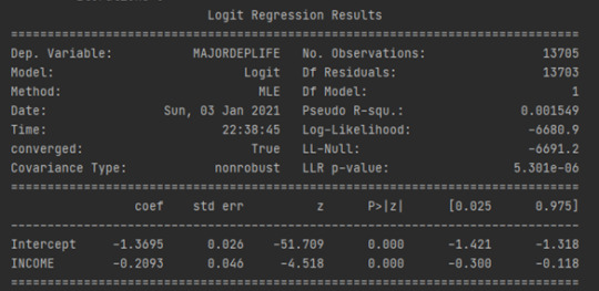
Notice also that our regression is significant at a P value of less than 0.05. Using the prime assessments, we could generate the linear equation. Major depression is a function of 0.026 plus 0.046 times Income but let's really think about the equation some more.

In a regression module, our response variable was quantitative. And so, it could theoretically take on any value. In a logistic regression, our response variable only takes on the values zero and one. Therefore, if I try to use this equation as a best fit line, I would run into some problems.

Instead of talking in decimals it may be more helpful for us to talk about how the probability of being Major depression changes based on the Income level. Instead of true expected values, we want probabilities using our logistics regression model through Odds ratios:

By definition: The odds ratio is the probability of an event occurring in one group compared to the probability of an event occurring in another group. Odds ratios are always given in the form of odds and are not linear. The odds ratio is the natural exponentiation of our parameter estimate. Thus, all that we need to do is calculate the natural log to the power of our parameter estimate. Here are my results:

ODDS RATIOS

Here are the results. Because both my explanatory and response variables in the model are binary, coded zero and one. I can interpret the odds ratio in the following way. Since it was less than 1 which is 0.81, High income young adults in my sample are 0.81 times less likely to have major depression than low income young adult.

CONFIDENCE INTERVALS

Looking at the confidence interval, we can get a better picture of how much this value would change for a different sample drawn from the population. Based on our model, high income young adults are anywhere from 0.74 to 0.89 times less likely to have major depression than those low income young adults. The odds ratio is a sample statistic and the confidence intervals are an estimate of the population parameter.

Now, I want to test a potential confounder to add in my model which is Gender. I’ve run another logistic regression with Gender as my potential confounder and here are the results:

LOGISTIC REGRESSION

As we can see, both Personal Income and Gender are independently associated with the likelihood of having major depression but they are negatively associated with a likelihood of having major depression. Gender is not a confounder between my Primary response variable and Primary explanatory variable.

ODDS RATIOS

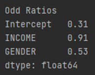
In our predictor or splinter variables are both binary, we can interpret the odds ratio in the following way. High income young adults in my sample are 0.91 times less likely to have major depression than low income young adult after controlling for major depression. Also, Male young adults in my sample are 0.53 times less likely to have major depression than Female young adult after controlling for major depression.

CONFIDENCE INTERVALS:

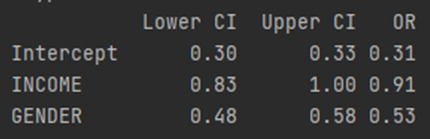
Because the confidence intervals on our odds ratios overlap, we cannot say that Personal income is more strongly associated with Major depression than Gender. For the population of High income young adults, we can say that those high income young adults are anywhere between 0.83 to 1 times less likely to have major depression than low income young adult. And those Male young adults are between 0.48 and 0.58 times less likely to have major depression than Female young adults. Both of these estimates are calculated after accounting for the alternate disorder. As with multiple regression, when using logistic regression, we can continue to add variables to our model in order to evaluate multiple predictors of our binary categorical response variable. Presence or absence of major depression.

My Python Code:

0 notes

engrflores · 4 years ago

Text

Regression Modeling in Practice

Regression Modeling in Practice - Week 3 (Test a Multiple Regression Model)

I’ve run a linear regression analysis between my Explanatory variable, Educational attainment and my Response variable, Personal Income. There is a significant value which is less than 0.5 and positive parameter estimate which means that there is a statistically positive significant association between my two variables.

Now, I want to test the association between Personal Income and Educational attainment between young adults as our sample, I would like to add another predictor variable in my regression analysis which is if the presence of Major depression. Since, major depression is categorical and 0 is already coded within it’s results, there’s no need for me to recode the said variable. Here are my multiple regression results:

Based on the output in my Explanatory variable, Educational attainment and my potential confounder, Major depression, we can see that their P-values are less than 0.05 which means that they are both associated with my response variable personal income after partialing out the part of the association that can be accounted for by the other. Educational attainment variable has positives parameter estimate while Major depression has negative parameter estimate. This means that Educational attainment is positively associated with the response variable Personal income after controlling for the variable Major depression and vice versa. This also mean that with high Educational attainment, Income increases and with the presence of major depression, income decreases.

I’ve included another 3 predictor variables in my model which is Age, Gender and Energy level. Age and Energy level are quantitative variable therefore I’ve centered it by subtracting it’s mean from the actual value from each observation which essentially centers the variable at zero. Gender is coded with 1=Male 2=Female, therefore, to center it, I’ve recoded it to 1=Male 0=Female. This are the results:

To get a better understanding of our sample estimates represent the population values, we can look at confidence intervals. Confident intervals tell us which values of the parameter estimates are plausible in the population.

Typically, we look at 95% confidence intervals which tell us with 95% certainty the range of parameter estimate values that includes the true population parameter. That is, we are 95% certain that the true population parameter falls somewhere between the lower and upper confidence limits that are estimated based on a sample parameter estimate.

The parameter estimate of Educational attainment is 1129.62 which means that 1129.62 more income between young adults with higher educational attainment on young adults than without.

If we look at the confidence interval with the same variable, we see that it ranges from 962.84 to 1296.4. Meaning that we're 95% certain, that the true population parameter for the association between Major depression, and Personal income fall somewhere between these values. That is, in the population, there's a 95% chance that people with higher Educational attainment have anywhere between 962.84 to 1296.4 more income than people without major depression.

By examining their P-values, Educational attainment, Major Depression, Gender and Age are significantly associated with personal income while only Energy level is not.

We can also see that our primary explanatory variable has a significant P-value which is we reject the null hypothesis that there is no association and accept the alternative hypothesis of there us an association between income and educational attainment after adjusting for primary explanatory variable, major depression and other explanatory variables in my model. There are no potential confounders in my model that confounds the relationship between my primary explanatory variable and response variable.

So far, we have used regression to test linear associations between our explanatory variables, and our response variable. By linear, we mean that the association can be explained best with a straight line.

Here is a scatter plot showing a linear association between Personal Income Educational Attainment.

That is, we can a draw a straight line to the scatter plot and this regression line does a pretty good job of catching the association.

Having limited values in my Explanatory and Response variables with more the 4,000 of observations, my scatter plot looks like this but still we can gain information on it by seeing that there is a positive linear relationship between the two. This means that, when Educational Attainment is high, Personal income will also be high.

By looking at my linear scatter plot above, I am confident that this line is the best fit for my data but I will still test by adding a polynomial term to compare the results within the two that best fits. And here is the result:

Now my scatterplot shows the original linear regression line in blue, and the quadratic regression line in orange. Based on just looking at the two curves, it still not clear to me which is the best fit for the data. Now, I can be sure I test to see whether adding a second order polynomial term to our aggression model gives us a significantly better fitting model. I do this by simply adding another variable that is the squared value of my explanatory x variable, x squared, to my regression model.

Based on the regression model results I have earlier for just the linear association between Personal Income and Educational attainment, there is a significant value which is less than 0.5 and positive parameter estimate which means that there is a statistically positive significant association between my two variables. But the R-square is only 0.05 which means that only 5% of the variability of the response variable can be predicted by the explanatory variable.

Therefore, I will try to add a second order polynomial to that regression equation and these are the results:

When we look at the table of results, by adding a quadratic term to our model we see that the P-value for our linear term is more than 0.05 which is statistically insignificant. Notice that there is a very small change in our R-squared which doesn’t increase the amount of variability in our response variable that can be explained by our explanatory variable. Together, these results suggest that the best fitting line for this association is one that includes linear.

In this regression model, the residual is the difference between the expected or predicted female employment rate, and the actual observed female employment rate for each country. We can take a look at this residual variability, which not only helps us to see how large the residuals are, but also allows us to see whether our regression assumptions are met. And whether there are any outlying observations, that might be unduly influencing the estimation of the regression coefficient.

The easiest way to evaluate residuals, is to graph them. First, we can use a qq-plot to evaluate the assumption that the residuals from our aggression model are normally distributed.

QQ-PLOT

A qq-plot, plots the quantiles of the residuals that we would theoretically see if the residuals followed a normal distribution, against the quantiles for the residuals estimated from our aggression model.

The qqplot for our regression model residuals deviates and does not follow a straight line. This indicates that our residuals did not follow perfect normal distribution. There might be other explanatory variables that we might consider including in our model, that could improve estimation of the observed curvilinearity.

STANDARDIZED RESIDUALS

In terms of evaluating the overall fit of the model, there are lots of my residuals that exceeded an absolute value of 2.5. This suggests that the fit of the model is relatively poor and could be improved. In order to improve the fit of this model, we should include more explanatory variables to better explain the variability in our Personal Income response variable.

The following plots help us determine how specific explanatory variables contribute to the fit of our model. In this example we're examining the Age explanatory variable but we can also look at these plots for other explanatory variables.

The primary plots of interest are the plots of the residuals for each observation of different of values of Age in the upper right hand corner and partial regression plot which is in the lower left hand corner.

This plot shows the residuals for each observation at different values of mean Age. There’s not a clearly pattern on it, as there is points all over the graph. But we can assume based on the plot that the absolute values of the residuals are significantly smaller at lower values of Age. But get larger as Educational attainment increases. But is particularly worse predicting Personal income for young adults with high Educational attainment.

Because we have multiple explanatory variables, we might want to take a look at the contribution of each individual explanatory variable to model fit, controlling for the other explanatory variables. One type of plot that does this, is the partial regression residual plot. It attempts to show the effect of adding mean Age as an additional explanatory variable to the model. Given that one or more explanatory variables are already in the model. For the Age variable, the values in the scatter plot are two sets of residuals. The residuals from a model predicting the Personal Income response from the other explanatory variables, excluding mean Age, are plotted on the vertical access, and the residuals from the model predicting mean Age from all the other explanatory variables are plotted on the horizontal access. What this means is that the partial regression plot shows the relationship between the response variable and specific explanatory variable, after controlling for the other explanatory variables. We can examine the plot to see if the mean Age residuals show a linear, or non-linear pattern. The partial regression plot for mean Age does not clearly indicate a linear association. Rather, the residuals are spread out in a random pattern around the partial regression line. In addition, many of the residuals are pretty far from this line, indicating a great deal of Personal income prediction error. This suggests that although Age shows a statistically significant association with Personal Income, this association is pretty weak after controlling for other explanatory variables. We can look at the partial regression residual plots for each of the other explanatory variables as well.

LEVERAGE PLOT

One of the first things we see in the leverage plot is that we have a many outliers which can be determined on contents that have residuals greater than 2 but this plot also tells us that these outliers have small or close to zero leverage values, meaning that although they are outlying observations, they do not have an undue influence on the estimation of the regression model.

My Python program:

import numpy as np import pandas as pd import statsmodels.api as sm import seaborn import statsmodels.formula.api as smf import matplotlib.pyplot as plt # bug fix for display formats to avoid run time errors pd.set_option('display.float_format', lambda x:'%.2f'%x) # load csv file data = pd.read_csv('NESARC_Data_Set.csv', low_memory=False) # convert values to numerical data['S1Q10A'] =pd.to_numeric(data['S1Q10A'], errors='coerce') data['MAJORDEPLIFE'] = pd.to_numeric(data['MAJORDEPLIFE'], errors='coerce') data['AGE']=pd.to_numeric(data['AGE'],errors='coerce') data['S1Q212']=pd.to_numeric(data['S1Q212'],errors='coerce') data['NMANDX12']=pd.to_numeric(data['NMANDX12'],errors='coerce') data['SEX']=pd.to_numeric(data['SEX'],errors='coerce') data['S1Q6A']=pd.to_numeric(data['S1Q6A'],errors='coerce') # subset data to age 20-25 and icome 0-100000 sub1 = data[(data['AGE'] >= 20) & (data['AGE'] <= 25) & (data['S1Q10A'] >= 0) & (data['S1Q10A'] <= 100000)] B1=sub1.copy() B1['S1Q212']=B1['S1Q212'].replace(9, np.nan) # replace values def INCOME (row): if row['S1Q10A']<=20000: return 1 elif row['S1Q10A']<=40000: return 2 elif row['S1Q10A']<=60000: return 3 elif row['S1Q10A']<=80000: return 4 elif row['S1Q10A']<=100000: return 5 sub1['INCOME'] = sub1.apply (lambda row: INCOME (row),axis=1) # recode values recode1= {1:20000,2:40000,3:60000,4:80000,5:100000} B1['INCOME']=sub1['INCOME'].map(recode1) # convert Income variable to numerical B1['INCOME'] = pd.to_numeric(B1['INCOME'], errors='coerce') # Frequency table for variables print('Counts for Major Depression, 1=Yes 0=No') chk1 = B1['MAJORDEPLIFE'].value_counts(sort=False, dropna=False) print(chk1) print('Total Personal Income') chk2 = B1['INCOME'].value_counts(sort=True, dropna=False) print(chk2) #center explanatory variables for regression analysis B1['AGE_c']= (B1['AGE'] - B1['AGE'].mean()) print(B1['AGE_c'].mean()) B1['PENERGY_c']= (B1['S1Q212'] - B1['S1Q212'].mean()) print(B1['PENERGY_c'].mean()) # rename variable to MDISORDER B1['MDISORDER']= B1['NMANDX12'] # recode explanatory variables to include 0 recode2 = {1:1,2:0} B1['GENDER'] = B1['SEX'].map(recode2) B1['ALCC'] = B1['S2AQ1'].map(recode2) recode3 = {1:0,2:1,3:2,4:3,5:4,6:5,7:6,8:7,9:8,10:9,11:10,12:11,13:12,14:13} B1['EDUC'] = B1['S1Q6A'].map(recode3) # linear regression analysis 1 reg1 = smf.ols('INCOME ~ EDUC', data=B1).fit() print (reg1.summary()) # linear regression analysis 2 reg2 = smf.ols('INCOME ~ EDUC + MAJORDEPLIFE', data=B1).fit() print(reg2.summary()) # linear regression analysis 3 reg3 = smf.ols('INCOME ~ EDUC + MAJORDEPLIFE + AGE_c + PENERGY_c + GENDER', data=B1).fit() print(reg3.summary()) # first order(linear) scatterplot scat1 = seaborn.regplot(x="EDUC", y="INCOME", scatter=True, data=B1) plt.xlabel('Educational Attainment') plt.ylabel('Personal Income') plt.title ('Scatterplot for the Association Between Personal Income and Educational Attainment') # fit second order polynomial # run the 2 scatterplots together to get both linear and second order fit lines scat1 = seaborn.regplot(x="EDUC", y="INCOME", scatter=True, order=2, data=B1) plt.xlabel('Educational Attainment') plt.ylabel('Personal Income') plt.title ('Scatterplot for the Association Between Personal Income and Educational Attainment') plt.show() # quadratic (polynomial) regression analysis reg4 = smf.ols('INCOME ~ EDUC + I(EDUC**2)', data=B1).fit() print (reg4.summary()) reg5 = smf.ols('INCOME ~ EDUC + MAJORDEPLIFE + AGE_c', data=B1).fit() #Q-Q plot for normality fig1 = sm.qqplot(reg5.resid, line='r') plt.show() # simple plot of residuals stdres = pd.DataFrame(reg5.resid_pearson) plt.plot(stdres, 'o', ls='None') l = plt.axhline(y=0, color='r') plt.ylabel('Standardized Residual') plt.xlabel('Observation Number') plt.show() # additional regression diagnostic plots fig2 = plt.figure(figsize=(12,8)) fig2 = sm.graphics.plot_regress_exog(reg5, "AGE_c", fig=fig2) plt.show() # leverage plot fig3=sm.graphics.influence_plot(reg5, size=8) plt.show()

0 notes

engrflores · 4 years ago

Text

Regression Modeling in Practice

Regression Modeling in Practice - Week 2 ( Test a Basic Linear Regression Model )

This week's assignment asks us to test a basic linear regression model for the association between our primary explanatory variable and a response variable. My explanatory variable is Major Depression which has two categories (1=YES,0=NO). Since it has already a value of 0 on one of it’s categories, there’s no need for me to recode my categorical explanatory variable. Explanatory variable is quantitative which is Personal income between young adults from $-$100000. My research question is, is lower personal income associated with having major depression. Here’s my frequency table between my two variables:

As expected, there are more individuals who don’t have major depression and as income increases, number of observation decreases.

Testing my two variables using python, these are my OLS Regression results:

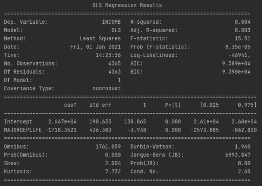
As we can see on the results, my Response variable income and my number of observations is 4365 which is young adults. The parameter estimate for INCOME is -1718.35 and the y-intercept is 26470. Thus, the equation looks like this:

INCOME = -1718.35(MAJORDEPLIFE) + 26470

I can plug the values of my Major depression which has the value of 1 which means it has major depression and 0 which means it does not have major depression to get the expected value of my personal income within each group.

INCOME = -1718.35(0) + 26470

INCOME = 26470

INCOME = -1718.35(1) + 26470

INCOME = 24751.65

As we could see, we can expect young adults with depression to have an income of 24751.65 and young adults without depression to have 26470.

We can therefore conclude that, income is associated with major depression between young adults.

My program:

0 notes

engrflores · 4 years ago

Text

Regression Modeling in Practice

Regression Modeling in Practice - Week 1 ( Writing About Your Data )

Sample:

The sample is from the first wave of the National Epidemiologic Survey on Alcohol and Related Conditions (NESARC), the largest nationwide longitudinal survey of alcohol and drug use and associated psychiatric and medical comorbidities. The sample of 3,629 young adults composed of low-income young adults ($0-$23,000) (n=3,435, 94.65%) and high-income young adults ($40000-$100000) (n=194, 5.35%). Young adults are been classified between ages 20-25 years old. Between low-income young adults 3,023 don’t have major depression and 412 has. On high-income young adults 187 don’t have major depression and only 7 has major depression.

Procedure:

Data were collected by trained U.S. Census Bureau Field Representatives during 2001– 2002 through computer-assisted personal interviews (CAPI). Sensitive questions such as personal income and major depression were asked using computer assisted interviewing to increase the reliability of responses.

Measures:

The measure of Major depression was drawn from the National Epidemiologic Survey on Alcohol and Related Conditions (NESARC), the largest nationwide longitudinal survey of alcohol and drug use and associated psychiatric and medical comorbidities. It measures between 3,629 young adults ages 20-25 years old with/without presence of major depression. For the current analysis, it was binned into two categories low-income ($0-$23,000) young adults and high-income ($40000-$100000) young adults.

0 notes

engrflores · 4 years ago

Text

Data Analysis Tools

Data Analysis Tools - Week 4 ( Testing a Potential Moderator )

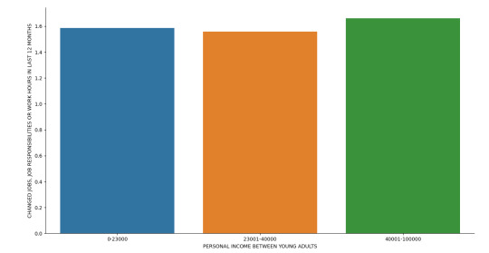
I test my explanatory variable Personal income between young adults and categorized it within 3 levels of income ranges which is from low income young adults ($0-$23000), average income young adults ($23001-$40000) and High income young adults ($40001-$100000) with my response variable Changed Jobs, Job responsibilities or work hours.

These two are both categorical variables therefore, I use a chi-square test of independence to test their relationship:

I have a large chi-square value and a significant p-value which tells us that they both have a significant relationship.

As we can also seen in our frequency table, low income group responded No with over 58% and over 66% between high income group. I have a lower income range in my average income group compared with the other groups that’s why there is a limited counts of respondents within this group. But overall, we can conclude that young adults don’t Change Jobs, Job responsibilities or work hours, as income increases.

To furtherly test the association between my two variables, I’ve added a third variable Had trouble with boss or coworker, which is my moderator that affects the direction and/or strength of their relation.

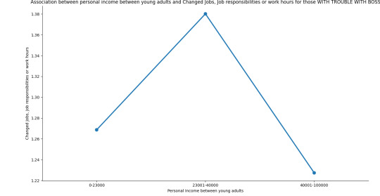
As we can see, the relationship between Personal income between young adults and Change Jobs, Job responsibilities or work hours depends if they Had trouble with boss or coworker or not.

As income increases between average income group and high income group without trouble with boss or coworker, they tend to favor not to Change Jobs, Job responsibilities or work hours.

As income increases between average income group and high income group with trouble with boss or coworker, they tend to favor to Change Jobs, Job responsibilities or work hours.

Therefore, we can say that there is a statistical interaction within these two variables when moderated by our third variable.

My Program:

import pandas as pd import numpy as np import scipy.stats import seaborn import matplotlib.pyplot as plt data = pd.read_csv('NESARC_Data_Set.csv', low_memory=False) #CONVERT TO NUMERIC data['S1Q10A']=data['S1Q10A'].apply(pd.to_numeric, errors='coerce') data['S1Q237']=data['S1Q237'].apply(pd.to_numeric, errors='coerce') #Data for Total Personal Income in the last 12 months (Ages 20-25) (Income between 0=25000$) sub1 = data[(data['AGE'] >= 20) & (data['AGE'] <= 25) & (data['S1Q10A'] >= 0) & (data['S1Q10A'] <= 100000)] B1 = sub1.copy() # recode missing values to python missing (NaN) B1['S1Q237']=B1['S1Q237'].replace(9, np.nan) def INRANGE (row): if row['S1Q10A'] <= 23000: return 1 elif row['S1Q10A'] <= 40000: return 2 elif row['S1Q10A'] <= 100000: return 3 B1['INRANGE'] = B1.apply (lambda row: INRANGE (row),axis=1) #recoding values for S1Q10A recode1 = {1: "0-23000", 2: "23001-40000", 3: "40001-100000"} B1['INRANGE']= B1['INRANGE'].map(recode1) # contingency table of observed counts ct1=pd.crosstab(B1['S1Q237'], B1['INRANGE']) print (ct1) # column percentages colsum=ct1.sum(axis=0) colpct=ct1/colsum print(colpct) # chi-square print ('chi-square value, p value, expected counts') cs1= scipy.stats.chi2_contingency(ct1) print (cs1) # set variable types B1["INRANGE"] = B1['INRANGE'].astype('category') B1['S1Q237'] = B1['S1Q237'].apply(pd.to_numeric, errors='coerce') # bivariate bar graph seaborn.factorplot(x="INRANGE", y="S1Q237", data=B1, kind="bar", ci=None) plt.xlabel('PERSONAL INCOME BETWEEN YOUNG ADULTS') plt.ylabel('CHANGED JOBS, JOB RESPONSIBILITIES OR WORK HOURS IN LAST 12 MONTHS') plt.show() sub3=B1[(B1['S1Q236']== 2)] sub4=B1[(B1['S1Q236']== 1)] print ('Association between personal income between young adults and Changed Jobs, Job responsibilities or work hours for those W/O TROUBLE WITH BOSS') # contingency table of observed counts ct2=pd.crosstab(sub3['S1Q237'], sub3['INRANGE']) print (ct2) # column percentages colsum=ct1.sum(axis=0) colpct=ct1/colsum print(colpct) # chi-square print ('chi-square value, p value, expected counts') cs2= scipy.stats.chi2_contingency(ct2) print (cs2) print ('Association between personal income between young adults and Changed Jobs, Job responsibilities or work hours for those WITH TROUBLE WITH BOSS') # contingency table of observed counts ct3=pd.crosstab(sub4['S1Q237'], sub4['INRANGE']) print (ct3) # column percentages colsum=ct1.sum(axis=0) colpct=ct1/colsum print(colpct) # chi-square print ('chi-square value, p value, expected counts') cs3= scipy.stats.chi2_contingency(ct3) print (cs3) seaborn.factorplot(x="INRANGE", y="S1Q237", data=sub4, kind="point", ci=None) plt.xlabel('Personal Income between young adults') plt.ylabel('Changed Jobs, Job responsibilities or work hours') plt.title('Association between personal income between young adults and Changed Jobs, Job responsibilities or work hours for those WITH TROUBLE WITH BOSS') plt.show() seaborn.factorplot(x="INRANGE", y="S1Q237", data=sub3, kind="point", ci=None) plt.xlabel('Personal Income between young adults') plt.ylabel('Changed Jobs, Job responsibilities or work hours') plt.title('Association between personal income between young adults and Changed Jobs, Job responsibilities or work hours for those WITHOUT TROUBLE WITH BOSS') plt.show()

0 notes

engrflores · 4 years ago

Text

Data Analysis Tools

Data Analysis Tools - Week 3 (Generating a Correlation Coefficient)

I’ve test if there is an association between my Quantitative Explanatory variable Age and Quantitative Response variable Weight (lbs) using the Pearson Correlation test. Running my program in python, these are the results:

My correlation coefficient tells us that it has a weak relationship because is close to zero and also has a non-significant P value which is greater than our significance level of 0.05 .

As we can see on my scatterplot between the relationship between Age and Weight, it creates a curvilinear relationship, we can see that at ages 20-60 there is a slightly increase in the weight and then decreases rapidly between ages 60-90. As we interpret on our results using the Pearson correlation test, the correlation is useless for accessing the strength of any type of relationship that is not linear including relationships that are curvilinear. However, we can tell that this is a weak linear relationship.

We can look at the P value to determine if there is an association between two variables. Our P-value is much greater than our significance level which means it is not significant.

When we square our correlation coefficient we get our small r squared (or Coefficient of determination) which can get the fraction of variability of one variable that can be predicted by the other. In my case, (0.055)^2=0.003 which is If we know the Age, we can predict 0.3% of the variability we will see in the Weight.

My python program:

0 notes

engrflores · 4 years ago

Text

Data Analysis Tools

Data Analysis Tools - Week 2 ( Running a Chi-Square Test of Independence )

When examining the association between lifetime major depression (categorical response) and low income young adults (categorical explanatory), a chi-square test of independence was used among low income, young adults (my sample). There is no clear pattern on my data to reject the null hypothesis and accept the alternative hypothesis. However, looking at the chi-square result, the chi-square value is large with 15.67 and a smaller value than our cut-off point with 0.028 which tells us that there is an association between major depression and personal income.

Here is the graph between Income between young adults and major depression which there is no significant pattern that we can conclude to reject the null hypothesis.

Post hoc tests for Chi Square tests

Since my Categorical Explanatory variable has 8 levels, I perform a post hoc test known as the Bonferroni Adjustment to control the family-wise error rate, also known as the maximum overall type I error rate, so that we can evaluate which pairs of major depression rates are different from one another.

The process would be to conduct each of the 15 paired comparisons. But rather than evaluating significance at the P 0.05 level, we would adjust the P value to make it more difficult to reject the null hypothesis. The adjusted P value is calculated by dividing P 0.05 by the number of comparisons which is in my case is 28. Therefore, my adjusted P value level is now 0.05/28=0.00178.

Summary of Post hoc tests between pair:

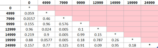
As we can see in the table, all of the P values of my categorical pairs are above the adjusted P value which is 0.00178. We can conclude on our Chi-square test that our data do not have significantly different rates of major depression. Therefore, we fail to reject the null Hypothesis.

My Program:

import numpy as np import pandas as pd import scipy.stats import seaborn import matplotlib.pyplot as plt data=pd.read_csv("NESARC_Data_Set.csv",low_memory=False) #Data for Total Personal Income in the last 12 months (Ages 20-25) (Income between 0=25000$) A1 = data[(data['AGE'] >= 20) & (data['AGE'] <= 25) & (data['S1Q10B'] >= 0) & (data['S1Q10B'] <= 7)] B1 = A1.copy() recode= {0:0,1:4999,2:7999,3:9999,4:12999,5:14999,6:19999,7:24999} B1['INCOMERANGE']=B1['S1Q10B'].map(recode) d1=B1['INCOMERANGE'].value_counts(sort=False) # contingency table of observed counts ct1=pd.crosstab(B1['DMAJORDEPSNI12'], B1['INCOMERANGE']) print (ct1) # column percentages colsum=ct1.sum(axis=0) colpct=ct1/colsum print(colpct) # chi-square print('chi-square value, p value, expected counts') cs1= scipy.stats.chi2_contingency(ct1) print(cs1) # set variable types B1['INCOMERANGE'] = B1['INCOMERANGE'].astype('category') B1['DMAJORDEPSNI12'] = pd.to_numeric(B1['DMAJORDEPSNI12'], errors='coerce') # graph percent with nicotine dependence within each smoking frequency group seaborn.barplot(x="INCOMERANGE", y="DMAJORDEPSNI12", data=B1) plt.xlabel('Income between Young adults') plt.ylabel('Major Depression') plt.show() recode2 = {0: 0, 4999: 4999} B1['COMP0v4999']= B1['INCOMERANGE'].map(recode2) # contingency table of observed counts ct2=pd.crosstab(B1['DMAJORDEPSNI12'], B1['COMP0v4999']) print(ct2) # column percentages colsum=ct2.sum(axis=0) colpct=ct2/colsum print(colpct) print('chi-square value, p value, expected counts') cs2= scipy.stats.chi2_contingency(ct2) print(cs2) recode3 = {0: 0, 7999: 7999} B1['COMP0v7999']= B1['INCOMERANGE'].map(recode3) # contingency table of observed counts ct3=pd.crosstab(B1['DMAJORDEPSNI12'], B1['COMP0v7999']) print(ct3) # column percentages colsum=ct3.sum(axis=0) colpct=ct3/colsum print(colpct) print('chi-square value, p value, expected counts') cs3= scipy.stats.chi2_contingency(ct3) print(cs3) recode4 = {0: 0, 9999: 9999} B1['COMP0v9999']= B1['INCOMERANGE'].map(recode4) # contingency table of observed counts ct4=pd.crosstab(B1['DMAJORDEPSNI12'], B1['COMP0v9999']) print(ct4) # column percentages colsum=ct4.sum(axis=0) colpct=ct4/colsum print(colpct) print('chi-square value, p value, expected counts') cs4= scipy.stats.chi2_contingency(ct4) print(cs4) recode5 = {0: 0, 12999: 12999} B1['COMP0v12999']= B1['INCOMERANGE'].map(recode5) # contingency table of observed counts ct5=pd.crosstab(B1['DMAJORDEPSNI12'], B1['COMP0v12999']) print(ct5) # column percentages colsum=ct5.sum(axis=0) colpct=ct5/colsum print(colpct) print('chi-square value, p value, expected counts') cs5= scipy.stats.chi2_contingency(ct5) print(cs5) recode6 = {0: 0, 14999: 14999} B1['COMP0v14999']= B1['INCOMERANGE'].map(recode6) # contingency table of observed counts ct6=pd.crosstab(B1['DMAJORDEPSNI12'], B1['COMP0v14999']) print(ct6) # column percentages colsum=ct6.sum(axis=0) colpct=ct6/colsum print(colpct) print ('chi-square value, p value, expected counts') cs6= scipy.stats.chi2_contingency(ct6) print(cs6) recode7 = {0: 0, 19999: 19999} B1['COMP0v19999']= B1['INCOMERANGE'].map(recode7) # contingency table of observed counts ct7=pd.crosstab(B1['DMAJORDEPSNI12'], B1['COMP0v19999']) print(ct7) # column percentages colsum=ct7.sum(axis=0) colpct=ct7/colsum print(colpct) print ('chi-square value, p value, expected counts') cs7=scipy.stats.chi2_contingency(ct7) print(cs7) recode8 = {0: 0, 24999: 24999} B1['COMP0v24999']= B1['INCOMERANGE'].map(recode8) # contingency table of observed counts ct8=pd.crosstab(B1['DMAJORDEPSNI12'], B1['COMP0v24999']) print(ct8) # column percentages colsum=ct8.sum(axis=0) colpct=ct8/colsum print(colpct) print ('chi-square value, p value, expected counts') cs8=scipy.stats.chi2_contingency(ct8) print(cs8) recode9 = {4999: 4999, 7999: 7999} B1['COMP4999v7999']= B1['INCOMERANGE'].map(recode9) # contingency table of observed counts ct9=pd.crosstab(B1['DMAJORDEPSNI12'], B1['COMP4999v7999']) print(ct9) # column percentages colsum=ct9.sum(axis=0) colpct=ct9/colsum print(colpct) print ('chi-square value, p value, expected counts') cs9=scipy.stats.chi2_contingency(ct9) print(cs9) recode10 = {4999: 4999, 9999: 9999} B1['COMP4999v9999']= B1['INCOMERANGE'].map(recode10) # contingency table of observed counts ct10=pd.crosstab(B1['DMAJORDEPSNI12'], B1['COMP4999v9999']) print(ct10) # column percentages colsum=ct10.sum(axis=0) colpct=ct10/colsum print(colpct) print ('chi-square value, p value, expected counts') cs10=scipy.stats.chi2_contingency(ct10) print(cs10) recode11 = {4999: 4999, 12999: 12999} B1['COMP4999v12999']= B1['INCOMERANGE'].map(recode11) # contingency table of observed counts ct11=pd.crosstab(B1['DMAJORDEPSNI12'], B1['COMP4999v12999']) print(ct11) # column percentages colsum=ct11.sum(axis=0) colpct=ct11/colsum print(colpct) print ('chi-square value, p value, expected counts') cs11=scipy.stats.chi2_contingency(ct11) print(cs11) recode12 = {4999: 4999, 14999: 14999} B1['COMP4999v14999']= B1['INCOMERANGE'].map(recode12) # contingency table of observed counts ct12=pd.crosstab(B1['DMAJORDEPSNI12'], B1['COMP4999v14999']) print(ct12) # column percentages colsum=ct12.sum(axis=0) colpct=ct12/colsum print(colpct) print ('chi-square value, p value, expected counts') cs12=scipy.stats.chi2_contingency(ct12) print(cs12) recode13 = {4999: 4999, 19999: 19999} B1['COMP4999v19999']= B1['INCOMERANGE'].map(recode13) # contingency table of observed counts ct13=pd.crosstab(B1['DMAJORDEPSNI12'], B1['COMP4999v19999']) print(ct13) # column percentages colsum=ct13.sum(axis=0) colpct=ct13/colsum print(colpct) print ('chi-square value, p value, expected counts') cs13=scipy.stats.chi2_contingency(ct13) print(cs13) recode14 = {4999: 4999, 24999: 24999} B1['COMP4999v24999']= B1['INCOMERANGE'].map(recode14) # contingency table of observed counts ct14=pd.crosstab(B1['DMAJORDEPSNI12'], B1['COMP4999v24999']) print(ct14) # column percentages colsum=ct14.sum(axis=0) colpct=ct14/colsum print(colpct) print ('chi-square value, p value, expected counts') cs14=scipy.stats.chi2_contingency(ct14) print(cs14) recode15 = {7999: 7999, 9999: 9999} B1['COMP7999v9999']= B1['INCOMERANGE'].map(recode15) # contingency table of observed counts ct15=pd.crosstab(B1['DMAJORDEPSNI12'], B1['COMP7999v9999']) print(ct15) # column percentages colsum=ct15.sum(axis=0) colpct=ct15/colsum print(colpct) print ('chi-square value, p value, expected counts') cs15=scipy.stats.chi2_contingency(ct15) print(cs15) recode16 = {7999: 7999, 12999: 12999} B1['COMP7999v12999']= B1['INCOMERANGE'].map(recode16) # contingency table of observed counts ct16=pd.crosstab(B1['DMAJORDEPSNI12'], B1['COMP7999v12999']) print(ct16) # column percentages colsum=ct16.sum(axis=0) colpct=ct16/colsum print(colpct) print ('chi-square value, p value, expected counts') cs16=scipy.stats.chi2_contingency(ct16) print(cs16) recode17 = {7999: 7999, 14999: 14999} B1['COMP7999v14999']= B1['INCOMERANGE'].map(recode17) # contingency table of observed counts ct17=pd.crosstab(B1['DMAJORDEPSNI12'], B1['COMP7999v14999']) print(ct17) # column percentages colsum=ct17.sum(axis=0) colpct=ct17/colsum print(colpct) print ('chi-square value, p value, expected counts') cs17=scipy.stats.chi2_contingency(ct16) print(cs17) recode18 = {7999: 7999, 19999: 19999} B1['COMP7999v19999']= B1['INCOMERANGE'].map(recode18) # contingency table of observed counts ct18=pd.crosstab(B1['DMAJORDEPSNI12'], B1['COMP7999v19999']) print(ct18) # column percentages colsum=ct18.sum(axis=0) colpct=ct18/colsum print(colpct) print ('chi-square value, p value, expected counts') cs18=scipy.stats.chi2_contingency(ct16) print(cs18) recode19 = {7999: 7999, 24999: 24999} B1['COMP7999v24999']= B1['INCOMERANGE'].map(recode19) # contingency table of observed counts ct19=pd.crosstab(B1['DMAJORDEPSNI12'], B1['COMP7999v24999']) print(ct19) # column percentages colsum=ct19.sum(axis=0) colpct=ct19/colsum print(colpct) print ('chi-square value, p value, expected counts') cs19=scipy.stats.chi2_contingency(ct19) print(cs19) recode20 = {9999: 9999, 12999: 12999} B1['COMP9999v12999']= B1['INCOMERANGE'].map(recode20) # contingency table of observed counts ct20=pd.crosstab(B1['DMAJORDEPSNI12'], B1['COMP9999v12999']) print(ct20) # column percentages colsum=ct20.sum(axis=0) colpct=ct20/colsum print(colpct) print ('chi-square value, p value, expected counts') cs20=scipy.stats.chi2_contingency(ct20) print(cs20) recode21 = {9999: 9999, 14999: 14999} B1['COMP9999v14999']= B1['INCOMERANGE'].map(recode21) # contingency table of observed counts ct21=pd.crosstab(B1['DMAJORDEPSNI12'], B1['COMP9999v14999']) print(ct21) # column percentages colsum=ct21.sum(axis=0) colpct=ct21/colsum print(colpct) print ('chi-square value, p value, expected counts') cs21=scipy.stats.chi2_contingency(ct21) print(cs21) recode22 = {9999: 9999, 19999: 19999} B1['COMP9999v19999']= B1['INCOMERANGE'].map(recode22) # contingency table of observed counts ct22=pd.crosstab(B1['DMAJORDEPSNI12'], B1['COMP9999v19999']) print(ct22) # column percentages colsum=ct22.sum(axis=0) colpct=ct22/colsum print(colpct) print ('chi-square value, p value, expected counts') cs22=scipy.stats.chi2_contingency(ct22) print(cs22) recode23 = {9999: 9999, 24999: 24999} B1['COMP9999v24999']= B1['INCOMERANGE'].map(recode23) # contingency table of observed counts ct23=pd.crosstab(B1['DMAJORDEPSNI12'], B1['COMP9999v24999']) print(ct23) # column percentages colsum=ct23.sum(axis=0) colpct=ct23/colsum print(colpct) print ('chi-square value, p value, expected counts') cs23=scipy.stats.chi2_contingency(ct23) print(cs23) recode24 = {12999: 12999, 14999: 14999} B1['COMP12999v14999']= B1['INCOMERANGE'].map(recode24) # contingency table of observed counts ct24=pd.crosstab(B1['DMAJORDEPSNI12'], B1['COMP12999v14999']) print(ct24) # column percentages colsum=ct24.sum(axis=0) colpct=ct24/colsum print(colpct) print ('chi-square value, p value, expected counts') cs24=scipy.stats.chi2_contingency(ct24) print(cs24) recode25 = {12999: 12999, 19999: 19999} B1['COMP12999v19999']= B1['INCOMERANGE'].map(recode25) # contingency table of observed counts ct25=pd.crosstab(B1['DMAJORDEPSNI12'], B1['COMP12999v19999']) print(ct25) # column percentages colsum=ct25.sum(axis=0) colpct=ct25/colsum print(colpct) print ('chi-square value, p value, expected counts') cs25=scipy.stats.chi2_contingency(ct25) print(cs25) recode26 = {12999: 12999, 24999: 24999} B1['COMP12999v24999']= B1['INCOMERANGE'].map(recode26) # contingency table of observed counts ct26=pd.crosstab(B1['DMAJORDEPSNI12'], B1['COMP12999v24999']) print(ct26) # column percentages colsum=ct26.sum(axis=0) colpct=ct26/colsum print(colpct) print ('chi-square value, p value, expected counts') cs26=scipy.stats.chi2_contingency(ct26) print(cs26) recode27 = {14999: 14999, 19999: 19999} B1['COMP14999v19999']= B1['INCOMERANGE'].map(recode27) # contingency table of observed counts ct27=pd.crosstab(B1['DMAJORDEPSNI12'], B1['COMP14999v19999']) print(ct27) # column percentages colsum=ct27.sum(axis=0) colpct=ct27/colsum print(colpct) print ('chi-square value, p value, expected counts') cs27=scipy.stats.chi2_contingency(ct27) print(cs27) recode28 = {14999: 14999, 24999: 24999} B1['COMP14999v24999']= B1['INCOMERANGE'].map(recode28) # contingency table of observed counts ct28=pd.crosstab(B1['DMAJORDEPSNI12'], B1['COMP14999v24999']) print(ct28) # column percentages colsum=ct28.sum(axis=0) colpct=ct28/colsum print(colpct) print ('chi-square value, p value, expected counts') cs28=scipy.stats.chi2_contingency(ct28) print(cs28) recode29 = {19999: 19999, 24999: 24999} B1['COMP19999v24999']= B1['INCOMERANGE'].map(recode29) # contingency table of observed counts ct29=pd.crosstab(B1['DMAJORDEPSNI12'], B1['COMP19999v24999']) print(ct29) # column percentages colsum=ct29.sum(axis=0) colpct=ct29/colsum print(colpct) print ('chi-square value, p value, expected counts') cs29=scipy.stats.chi2_contingency(ct29) print(cs29)

0 notes

engrflores · 4 years ago

Text

Data Analysis Tools

Data Analysis Tools - Week 1 ( Running an analysis of variance )

My Program:

import numpy as np import pandas as pd import statsmodels.formula.api as smf import statsmodels.stats.multicomp as multi data=pd.read_csv("NESARC_Data_Set.csv",low_memory=False) #Data for Total Personal Income in the last 12 months (Ages 20-25) (Income between 0=25000$) A1 = data[(data['AGE'] >= 20) & (data['AGE'] <= 25) & (data['S1Q10B'] >= 0) & (data['S1Q10B'] <= 7)] B1 = A1.copy() recode= {0:0,1:4999,2:7999,3:9999,4:12999,5:14999,6:19999,7:24999} B1['INCOMERANGE']=B1['S1Q10B'].map(recode) d1=B1['INCOMERANGE'].value_counts(sort=False) #CONVERT TO NUMERIC B1['INCOMERANGE']=B1['INCOMERANGE'].apply(pd.to_numeric, errors='coerce') # using ols function for calculating the F-statistic and associated p value model1 = smf.ols(formula='INCOMERANGE ~ C(DMAJORDEPSNI12)', data=B1) results1 = model1.fit() print (results1.summary()) B2 = B1[['INCOMERANGE', 'DMAJORDEPSNI12']].dropna() print ('Means for INCOMERANGE by Major Depression status') m1= B2.groupby('DMAJORDEPSNI12').mean() print (m1) print ('Standard Deviations for INCOMERANGE by Major Depression status') sd1 = B2.groupby('DMAJORDEPSNI12').std() print (sd1)

Output:

When examining the association between low income young adults (quantitative response) and major depression in the last 12 months between young adults (categorical explanatory), an Analysis of Variance (ANOVA) revealed that among low income young adults (my sample), those young adults who said Yes, they are experiencing major depression reported lesser income (Mean=11730.31, s.d. ±7593.49) compared to those people who don’t experience major depression (Mean=11961.97, s.d. ±7712.05).

My F-statistic is 0.33 and my P-value is 0.566 which is much higher than our alpha therefore, we accept the null Hypothesis (Ho) that there is no association between low income young adults and major depression.

0 notes

engrflores · 4 years ago

Text

Data Management and Visualization

Data Management and Visualization - Week 4 ( Creating graphs)

Hello! I’m Engr. Armando Flores Jr. This is my fourth blog as part of my submission for the week 4 assignment for the Part 1 of 5 course in the Data Analysis and Interpretation Specialization. This is for my assignment evaluation and to track my success all throughout this specialization.

These are the graphs of my variables (univariate graphs):

It is obvious and fair to say based on the graph on my two variables: Total Personal income in the past 12 months' frequency and counts decreases on an income range of $40000-$100000. Comparing both income ranges, the vast majority of individual young American adults within this data are from $0-$23000.

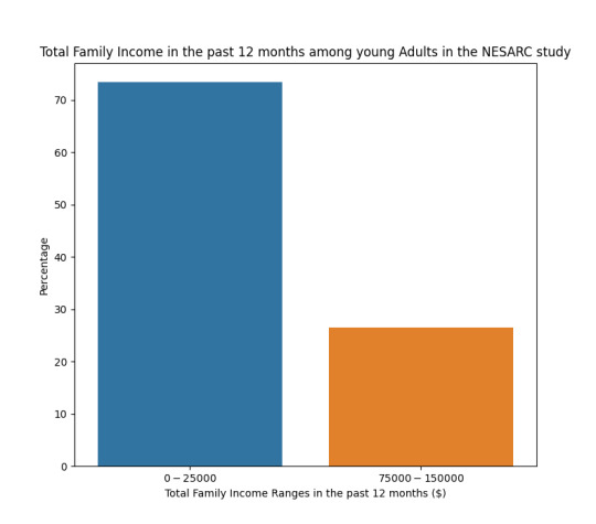
In the Total Family income in the past 12 months variable, frequency and percentage also decrease as we approach to a larger income range. more than 16000 families or around 70% in total of the data had an annual income of $0-$25000.

On my Became so restless that felt uncomfortable for 2+ weeks variable, High income young adults ($40000-$100000) had a slight decrease in percentage in the category who said 1 or YES compared to Low income young adults ($0-$23000).

On my Had trouble falling asleep nearly ever day for 2+ weeks variable, High income young adults ($40000-$100000) also had a slight decrease in percentage in the category who said 1 or YES compared to Low income young adults ($0-$23000).

Here, in my Histogram for Total personal Income in the last 12 months among young adults (age 20-25), as annual income increases, number of young adults decreases. It can be determined that a larger number of young adults had an income of $0-$23000. There are fewer who had an annual income of $40000-$100000.

Standard Deviation and other descriptive statistics for total personal income ($0-$100000) among young adults

Using the describe function in python, I was able to come up with these results on my quantitative variable. There are 4365 young adults who have an annual income between a minimum of 0$ and maximum of $100000. The Average annual income was $14647 and has a standard deviation of 12795. So, we can say that on average there are $14647 ± 12795 annual income.

Frequency of income ranges among young adults

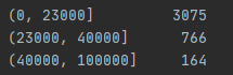
This data shows us the number of young adults who had a personal income out of these 3 income ranges. 3075 young adults had an annual income between $0-$23000, 766 had an annual income between $23000-$40000 and 164 had an annual income between $40000-$100000.

Creating my Explanatory and Response variables to form a C to C bar chart

Here, on the next graph, I want to fully examine if there is an association between Income and Depression. My Explanatory Independent Predictor variable Total Personal Income which is a quantitative variable under my first topic which is Income and my Response Dependent Outcome variable is Had trouble falling asleep nearly ever day for 2+ weeks which is a categorical variable under my second topic which is Depression. I’ve converted my explanatory variable into categorical in order to create a C to C bar chart with categories of income ranges from ($0-$23000), ($23000-$40000), ($40000-$100000). There are also two categories on my response variable which are coded 1 & 2 which 1 means YES or positive observation and 2 means NO or negative observation. Explanatory variable and Response Variable will be labeled on the x-axis and y-axis respectively on the Bivariate Graph.

Bivariate Graph

On my Bivariate graph, Income range of $0-$23000 has a mean proportion of 1.52. $23000-$40000 has a mean proportion of 1.6 and $40000-$100000 has a mean proportion of 1.68. We can observe from the graph that it creates an increasing pattern. This means that as salary range increases, there’s an increase on the response that says they Had no trouble falling asleep nearly every day for 2+ weeks.

Result:

This study was conducted during these pandemic where lots of individuals especially young adults who can’t find a job and some are laid off of by their current employers. Because of these, personal income was greatly affected that may lead to an impact on a person’s mental health that may lead to depression . There is an association between Income and Depression on young adults. Among young adults, there is an average of an annual income of $1464 which is inside my Low income range. These young adults are more prone to depression with their income at the lowest range. My Bivariate graph showed an increasing pattern that more High Income young adults had a negative response on my variables on Depression, meaning they didn’t experience any of these variables. Therefore, As income of an individual increases, the prevalence of lifetime depression then decreases.

My Python Code using Pycharm as text editor:

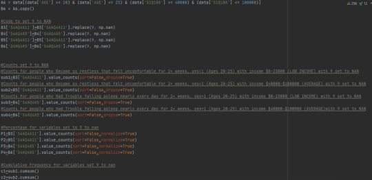
0 notes

engrflores · 4 years ago

Text

Data Management and Visualization

Data Management and Visualization - Week 3 ( Making Data Management Decisions)

Hello! I’m Engr. Armando Flores Jr. This is my third blog as part of my submission for the week 3 assignment for the Part 1 of 5 course in the Data Analysis and Interpretation Specialization. This is for my assignment evaluation and to track my success all throughout this specialization.

My Python Code using Pycharm as text editor:

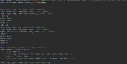
STEP 1: Make and implement data management decisions for the variables you selected.

I’ve code some valid data on my variables and separate those unknown data. I also group my variables. For example, on my Total Personal Income, I’ve divided it into two two make the data more simpler and easy to interpret, from low income young adults ($0-23000) and Average to High income young adults ($40000-$100000). I also did the same to my Total Family Income variable, divided it into two, low income ($0-$25000) and Average to High Income ($75000-$150000). All income ranges chosen was based on my research and data from Business Insider, Pew Research Center, and CNBC.

The same goes for my variables Became so restless that felt uncomfortable for 2+ weeks and Had Trouble falling asleep nearly every day for 2+ weeks where I group them into two income ranges setting up only between young adults and I set my unknown values from 9 to nan and coding in valid data.

STEP 2: Run frequency distributions for your chosen variables and select columns, and possibly rows.

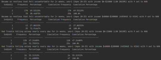
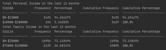
References:

https://www.businessinsider.com/income-amount-poverty-level-in-every-state-2018-11

https://www.pewsocialtrends.org/2020/01/09/trends-in-income-and-wealth-inequality/#:~:text=In%202018%2C%20the%20median%20income%20of%20U.S.%20households%20stood%20at%20%2474%2C600.&text=This%20was%2049%25%20higher%20than,the%20median%20income%20was%20%2450%2C200.&text=(Incomes%20are%20expressed%20in%202018%20dollars.)

https://www.cnbc.com/2019/01/23/how-much-money-americans-think-you-need-to-make-to-be-rich.html

0 notes

engrflores · 4 years ago

Text

Data Management and Visualization

Data Management and Visualization - Week 2 (My Python Program)

Hello! I’m Engr. Armando Flores Jr. This is my second blog as part of my submission for the week 2 assignment for the Part 1 of 5 course in the Data Analysis and Interpretation Specialization. This is for my assignment evaluation and to track my success all throughout this specialization.

My Python Code using Pycharm as text editor:

Frequency distribution for Total Personal Income ($) in the last 12 months (Ages 20-25) & (0$-40000$):

Frequency distribution for Total Family Income ($) in the last 12 months (0$-80000$):

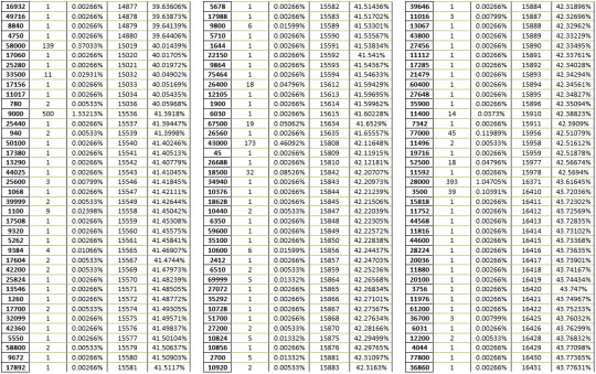
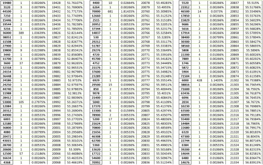
Frequency distribution for Became so restless that felt uncomfortable for 2+ weeks (Ages 20-25):

1. Yes 2. No 9. Unknown BL. NA, never or unknown if ever had period of low mood/when didn't care

Frequency distribution for Had Trouble falling asleep nearly every day for 2+ weeks (Ages 20-25):

From the Frequency distribution for Total Personal Income ($) in the last 12 months , there are 360 young adults said that they have no personal income with 8.56939% in total followed by 185 young adults who said that their total annual income is $12000 with 4.40371% in total.

From the Frequency distribution for Total Family Income ($) in the last 12 months , there are 1328 out of 3754 families said that their annual household income is $45000.

From the Frequency distribution for Became so restless that felt uncomfortable for 2+ weeks, there are 927 young adults with 21.21281% in total said 2 or No and 426 who said Yes.

From the Had Trouble falling asleep nearly every day for 2+ weeks, there are 693 young adults with 15.85812% in total said 2 or No and 661 who said Yes.

These are the following data that I’ve gathered and analyzed from NESARC data set from which I have selected four variables:

Total Personal Income in the last 12 months

Total Family Income in the last 12 months

Became so restless that felt uncomfortable for 2+ weeks

Frequency distribution for Had Trouble falling asleep nearly every day for 2+ weeks.

Here, I’d reconstructed my research question based on a specific set of observations: Association between Income and depression on young adults (ages 20-25).

After a series of researching and reading, I’ve decided to limit my data based on a specific set of observations focusing on young adults. My age range of young adults is from 20-25 years old based from Young Adult Development Project where they have range of 18 to 22 or 18 to 25 between young adults.

I’ve also decided to limit my Total Personal income and Total Family Income range based on a set of average range between young individual and also family income. Since NESARC conducted it’s survey mainly on Americans, I’ve conducted a research about the average income between individual Americans and their family and found out based on Economic Policy Institute that the the median wage in 2019 is $19.33 per hour, which translates into about $40,000 per year for a full-time, full-year worker. So, I’ve limit my Personal Income range from $0 or no personal income up to $40000 per year. Based on the FINANCIAL SAMURAI, the mean household income was roughly $80,000 as of 2019. Therefore, I’ve also set my data limit on my Total Family income per year up to $80000.

In survey conducted by the CNBC. To be considered “rich,” most Americans say you need an annual income of about $100,000.

And on TheStreet, the lowest-earning 10% of full-time employees is roughly $22,204 a year.

As a young adult, I am interested between the impact of depression on young adults. In AT THE CROSSROADS, it talks about why young adults so prone to depression.

‘”Young adults’ lives are full of trials and tribulations and are an emotional rollercoaster than lasts for years. With emotional stress and sadness leading to the development of bad habits and depression, early adulthood is the time in which there is a high... “

So I’ve decided to limit my two variables on depression between young adults.

Became so restless that felt uncomfortable for 2+ weeks, yes=1 (Ages 20-25) with income $0-23000 (LOW INCOME)

Became so restless that felt uncomfortable for 2+ weeks, yes=1 (Ages 20-25) with income $40000-$100000 (AVERAGE-HIGH INCOME)

Had Trouble falling asleep nearly every day for 2+ weeks, yes=1 (Ages 20-25) with income $0-23000 (LOW INCOME)

Had Trouble falling asleep nearly every day for 2+ weeks, yes=1 (Ages 20-25) with income $40000-$100000 (AVERAGE-HIGH INCOME)

Here, I’ve compared my variables to determine the association between Income and Depression. I’ve divided my variables within two categories which is Low income young adults ($0-$23000) and young adults who has an annual income which is from ($40000-$100000). In these tables, there are 972 low income young adults and 194 average-high income young adults. As you can see on the data above, average-high income young adults who said YES that they Became so restless that felt uncomfortable for 2+ weeks had a lower Percentage compared to low income young adults who said yes and almost nothing changed to the percentage who said No. Also, average-high income young adults who said YES that they Had Trouble falling asleep nearly every day for 2+ weeks had a lower Percentage compared to low income young adults who said yes and almost nothing changed to the percentage who said No. This means that low income young adults suffers more depression than average-high income young adults.

Conclusion:

Income has a great impact on a person’s mental health that may lead to depression especially on young adults.

References:

https://hr.mit.edu/static/worklife/youngadult/changes.html#:~:text=Young%20adulthood%20(generally%20defined%20as,as%20mid%2D20s%20and%20older)

https://www.epi.org/publication/swa-wages-2019/

https://www.financialsamurai.com/the-average-household-income-in-america/

https://www.cnbc.com/2019/01/23/how-much-money-americans-think-you-need-to-make-to-be-rich.html

https://www.thestreet.com/personal-finance/average-income-in-us-14852178#:~:text=This%20is%20roughly%20%2422%2C204%20a,group%20with%20the%20highest%20income.

https://www.atthecrossroads.com/FeedItem/Why-Are-Young-Adults-So-Prone-to-Depression/

0 notes

engrflores · 5 years ago

Text

Data Management and Visualization - Week 1

Hello! I’m Engr. Armando Flores Jr. This is my first blog as part of my submission for the week 1 assignment for the Part 1 of 5 course in the Data Analysis and Interpretation Specialization. This is for my assignment evaluation and to track my success all throughout this specialization.

Assignment 1:

We are given 5 data sets to select with our own topic of interest along with two topics and variables.

STEP 1: Choose a data set that you would like to work with.

For this one, I chose the NESARC Data Set.

The National Epidemiologic Study of Alcohol Related Conditions (NESARC) is a random sample survey of the United States population conducted in two waves by researchers at the Laboratory of Epidemiology and Biometry of the National Institute on Alcohol Abuse and Alcoholism (NIAAA). NESARC I (2001–02) interviewed 43 093 individuals in the United States aged 18 years and older [1]. NESARC II (2004–05) re-interviewed 34 653 respondents from wave I [2].

STEP 2. Identify a specific topic of interest.

After looking through the codebook of NESARC, my specific topic of interest is all about Income.

STEP 3. Prepare a codebook of your own.

STEP 4: Identify a second topic that you would like to explore in terms of its association with your original topic.

The second topic that I would like to explore in terms of its association with my original topic is Depression.

STEP 5. Add questions/items/variables documenting this second topic to your personal codebook.

My Variables under Income is:

Personal Income in the last 12 months.

Family Income in the last 12 months.

My Variables under Depression is:

Became so restless that felt uncomfortable for 2+ weeks.

Had Trouble falling asleep nearly every day for 2+ weeks.

My Research questions are:

Is Income associated with depression?

Is Personal income associated with depression?

Is Family Income associated with depression?

STEP 6. Perform a literature review to see what research has been previously done on this topic.

From Association and Depression Association of America (ADAA)

At a personal level:

Poverty leads to physiologic responses to stress such as high blood pressure and high cortisol levels. With prolonged exposure to poverty, these responses turn into disruptions in brain functioning, which ultimately lead to both long-term physical and mental health consequences. According to the CDC, 8.7% of people who have incomes below the poverty level report severe psychological distress.1energy consumption per capita and per dollar of GDP is between 0.35 and 0.48.

On a family level:

Poverty causes stressors such as insecurity in food, housing, income, and more. These stressors can also cause an increased risk of mental health problems and substance abuse in the parents, which can lead to child abuse and neglect and in turn cause negative mental health impacts for the child. Low-income communities tend to have specific characterizations such as limited resources, poor houses, high crime and violence rates, and an inadequate school system, which are all associated with poor mental health outcomes

Reference: https://adaa.org/finding-help/low-income-communities

STEP 7. Based on your literature review, develop a hypothesis about what you believe the association might be between these topics.

Personal Income is mainly one of the reason of one’s depression. Study shows that prolonged exposure to poverty, these responses turn into disruptions in brain functioning, which ultimately lead to both long-term physical and mental health consequences.

Family income highly affects mental health that may lead to depression because of the fact that Low-income communities tend to have limited resources that may lead to poor mental health outcomes. A decrease in household income was also associated with an increased risk of incident mood, anxiety, or substance use disorders

1 note · View note