faresar

[faresar]

Running LASSO regression

parameters:

CRIM - per capita crime rate by town

ZN - proportion of residential land zoned for lots over 25,000 sq.ft.

INDUS - proportion of non-retail business acres per town.

CHAS - Charles River dummy variable (1 if tract bounds river; 0 otherwise)

NOX - nitric oxides concentration (parts per 10 million)

RM - average number of rooms per dwelling

AGE - proportion of owner-occupied units built prior to 1940

DIS - weighted distances to five Boston employment centres

RAD - index of accessibility to radial highways

TAX - full-value property-tax rate per $10,000

PTRATIO - pupil-teacher ratio by town

B - 1000(Bk - 0.63)^2 where Bk is the proportion of blacks by town

LSTAT - % lower status of the population

MEDV - Median value of owner-occupied homes in $1000's

target:

TAX - full-value property-tax rate per $10,000

Dataset

The Boston Housing Dataset

Code

[faresar]

Running a k-means Cluster Analysis

from google.colab import drive

drive.mount('/content/drive')

#import the librariesimport pandas as pd

import numpy as np

import osimport matplotlib.pyplot as plt

from sklearn.model_selection import train_test_split

from pandas import Series,DataFrame

from sklearn.cluster import KMeans

from sklearn import preprocessing

#change directory

os.chdir('/content/drive/MyDrive/MachineLearning/K_mean clustring')

#import csv_data from drive

data=pd.read_csv('tree_addhealth.csv')

#upper case from all dataframe columns name 

data.columns=map(str.upper,data.columns)

#clean oservation miss data

data_clean=data.dropna()

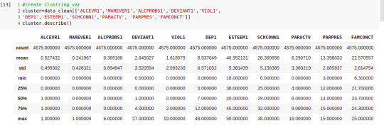
#create clustring var

cluster=data_clean[['ALCEVR1','MAREVER1','ALCPROBS1','DEVIANT1',

'VIOL1','DEP1','ESTEEM1','SCHCONN1','PARACTV','PARPRES','FAMCONCT']]

cluster.describe()

#standerlized clusring var for maen 0 and std 1

clustervar=cluster.copy() clustervar['ALCEVR1']=preprocessing.scale(clustervar['ALCEVR1']

.astype('float64')) clustervar['ALCPROBS1']=preprocessing.scale(clustervar['ALCPROBS1']

.astype('float64')) clustervar['MAREVER1']=preprocessing.scale(clustervar['MAREVER1']

.astype('float64')) clustervar['DEP1']=preprocessing.scale(clustervar['DEP1'].astype('float64')) clustervar['ESTEEM1']=preprocessing.scale(clustervar['ESTEEM1']

.astype('float64')) clustervar['VIOL1']=preprocessing.scale(clustervar['VIOL1'].astype('float64')) clustervar['DEVIANT1']=preprocessing.scale(clustervar['DEVIANT1']

.astype('float64')) clustervar['FAMCONCT']=preprocessing.scale(clustervar['FAMCONCT']

.astype('float64')) clustervar['SCHCONN1']=preprocessing.scale(clustervar['SCHCONN1']

.astype('float64')) clustervar['PARACTV']=preprocessing.scale(clustervar['PARACTV']

.astype('float64')) clustervar['PARPRES']=preprocessing.scale(clustervar['PARPRES']

.astype('float64'))

#split data to train_set and test_set

clust_train , clust_test= train_test_split(clustervar,test_size=.3,random_state=123)

# K_mean for 1-9 analysis

from scipy.spatial.distance import cdist clusters=range(1,10) meandist=[]

for k in clusters:    model=KMeans(n_clusters=k)    model.fit(clus_train)    clusassign=model.predict(clus_train)    meandist.append(sum(np.min(cdist(clus_train, model.cluster_centers_, 'euclidean'), axis=1))    / clus_train.shape[0])

""" Plot average distance from observations from the cluster centroid to use the Elbow Method to identify number of clusters to choose """

plt.plot(clusters, meandist) plt.xlabel('Number of clusters') plt.ylabel('Average distance') plt.title('Selecting k with the Elbow Method')

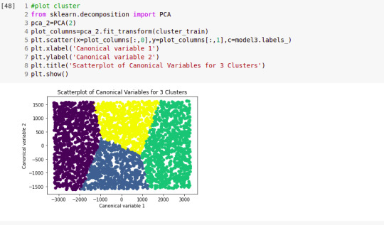
# Interpret 3 cluster solution model3=KMeans(n_clusters=3) model3.fit(clus_train) clusassign=model3.predict(clus_train) # plot clusters

from sklearn.decomposition import PCA pca_2 = PCA(2) plot_columns = pca_2.fit_transform(clus_train) plt.scatter(x=plot_columns[:,0], y=plot_columns[:,1], c=model3.labels_,) plt.xlabel('Canonical variable 1') plt.ylabel('Canonical variable 2') plt.title('Scatterplot of Canonical Variables for 3 Clusters') plt.show()

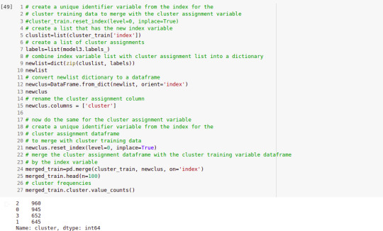
""" BEGIN multiple steps to merge cluster assignment with clustering variables to examine cluster variable means by cluster """ # create a unique identifier variable from the index for the # cluster training data to merge with the cluster assignment variable clus_train.reset_index(level=0, inplace=True) # create a list that has the new index variable cluslist=list(clus_train['index']) # create a list of cluster assignments labels=list(model3.labels_) # combine index variable list with cluster assignment list into a dictionary newlist=dict(zip(cluslist, labels)) newlist # convert newlist dictionary to a dataframe newclus=DataFrame.from_dict(newlist, orient='index') newclus # rename the cluster assignment column newclus.columns = ['cluster']

# now do the same for the cluster assignment variable # create a unique identifier variable from the index for the # cluster assignment dataframe # to merge with cluster training data newclus.reset_index(level=0, inplace=True) # merge the cluster assignment dataframe with the cluster training variable dataframe # by the index variable merged_train=pd.merge(clus_train, newclus, on='index') merged_train.head(n=100) # cluster frequencies merged_train.cluster.value_counts()

""" END multiple steps to merge cluster assignment with clustering variables to examine cluster variable means by cluster """

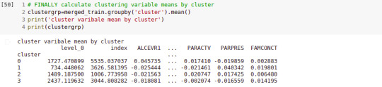
# FINALLY calculate clustering variable means by cluster clustergrp = merged_train.groupby('cluster').mean() print ("Clustering variable means by cluster") print(clustergrp)

# validate clusters in training data by examining cluster differences in GPA using ANOVA # first have to merge GPA with clustering variables and cluster assignment data gpa_data=data_clean['GPA1'] # split GPA data into train and test sets gpa_train, gpa_test = train_test_split(gpa_data, test_size=.3, random_state=123) gpa_train1=pd.DataFrame(gpa_train) gpa_train1.reset_index(level=0, inplace=True) merged_train_all=pd.merge(gpa_train1, merged_train, on='index') sub1 = merged_train_all[['GPA1', 'cluster']].dropna()

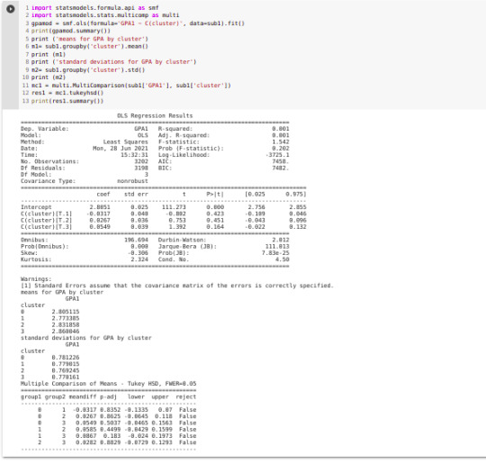
import statsmodels.formula.api as smf import statsmodels.stats.multicomp as multi

gpamod = smf.ols(formula='GPA1 ~ C(cluster)', data=sub1).fit() print (gpamod.summary())

print ('means for GPA by cluster') m1= sub1.groupby('cluster').mean() print (m1)

print ('standard deviations for GPA by cluster') m2= sub1.groupby('cluster').std() print (m2)

mc1 = multi.MultiComparison(sub1['GPA1'], sub1['cluster']) res1 = mc1.tukeyhsd() print(res1.summary())

[faresar]

#Running LASSO Regression Analysis

#import necessary libraries import pandas as pd import numpy as np import matplotlib.pylab as plt from sklearn.cross_validation import train_test_split from sklearn.linear_model import LassoLarsCV

#change directory path:

os.chdir('/content/drive/MyDrive/MachineLearning/Lasso Regression ')

#read csv_dataset from drive

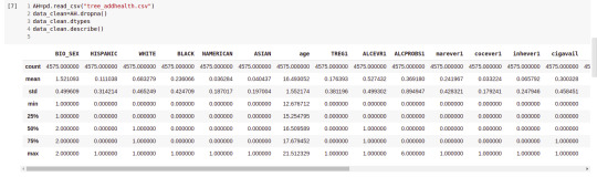
data=pd.read_csv('tree_addhealth.csv')

#upper_case for all dataframe column name

data.columns = map(str.upper, data.columns)

#Data managment for filtering male and female

data_clean = data.dropna()

recode1 = {1:1, 2:0}

data_clean['MALE']= data_clean['BIO_SEX'].map(recode1)

#select predictor variables and target variable as separate data sets  

predvar=data_clean[['MALE','HISPANIC','WHITE','BLACK','NAMERICAN','ASIAN','AGE','ALCEVR1','ALCPROBS1','MAREVER1','COCEVER1','INHEVER1','CIGAVAIL','DEP1','ESTEEM1','VIOL1','PASSIST','DEVIANT1','GPA1','EXPEL1','FAMCONCT','PARACTV','PARPRES']]

target = data_clean.SCHCONN1

#standardize predictors to have mean=0 and sd=1

predictors= predvar.copy()from sklearn import preprocessing predictors['MALE']=preprocessing.scale(predictors['MALE'].astype(’float64′))

predictors['HISPANIC']=preprocessing.scale(predictors['HISPANIC'].astype('float64'))

predictors['WHITE']=preprocessing.scale(predictors['WHITE'].astype('float64'))

predictors['NAMERICAN']=preprocessing.scale(predictors['NAMERICAN'].astype('float64'))

predictors['ASIAN']=preprocessing.scale(predictors['ASIAN'].astype('float64'))

predictors['AGE']=preprocessing.scale(predictors['AGE'].astype('float64'))

predictors['ALCEVR1']=preprocessing.scale(predictors['ALCEVR1'].astype('float64'))

predictors['ALCPROBS1']=preprocessing.scale(predictors['ALCPROBS1'].astype('float64'))

predictors['MAREVER1']=preprocessing.scale(predictors['MAREVER1'].astype('float64'))

predictors['COCEVER1']=preprocessing.scale(predictors['COCEVER1'].astype('float64'))

predictors['INHEVER1']=preprocessing.scale(predictors['INHEVER1'].astype('float64'))

predictors['CIGAVAIL']=preprocessing.scale(predictors['CIGAVAIL'].astype('float64'))

predictors['DEP1']=preprocessing.scale(predictors['DEP1'].astype('float64'))

predictors['ESTEEM1']=preprocessing.scale(predictors['ESTEEM1'].astype('float64'))

predictors['VIOL1']=preprocessing.scale(predictors['VIOL1'].astype('float64'))

predictors['PASSIST']=preprocessing.scale(predictors['PASSIST'].astype('float64'))

predictors['DEVIANT1']=preprocessing.scale(predictors['DEVIANT1'].astype('float64'))

predictors['GPA1']=preprocessing.scale(predictors['GPA1'].astype('float64'))

predictors['EXPEL1']=preprocessing.scale(predictors['EXPEL1'].astype('float64'))

predictors['FAMCONCT']=preprocessing.scale(predictors['FAMCONCT'].astype('float64'))

predictors['PARACTV']=preprocessing.scale(predictors['PARACTV'].astype('float64'))

predictors['PARPRES']=preprocessing.scale(predictors['PARPRES'].astype('float64'))

#split dataset to train=70% and test=30%

red_train,pred_test,tar_train,tar_test=train_test_split(predictors,target,test_size=0.3,random_state=123)

#specifiy LASSO Regression

model=LassoLarsCV(cv=10, precompute=False).fit(pred_train,tar_train)

#print variablet names after put in the lis and regression coefficients

dict(zip(predictors.columns,model.coef_))

#plot coefficient progression

m_log_alphas = -np.log10(model.alphas_)ax = plt.gca()plt.plot(m_log_alphas, model.coef_path_.T)

plt.axvline(-np.log10(model.alpha_), linestyle='--', color='k', label='alphaCV')

plt.ylabel('Regression Coefficients')

plt.xlabel('-log(alpha)')

plt.title('Regression Coefficients Progression for Lasso Paths')

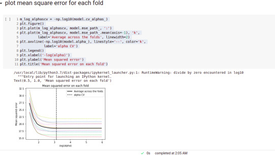
#plot mean square error for each fold

m_log_alphascv = -np.log10(model.cv_alphas_)

plt.figure()plt.plot(m_log_alphascv, model.mse_path_, ':')

plt.plot(m_log_alphascv, model.mse_path_.mean(axis=-1), 'k',  label='Average across the folds', linewidth=2)

plt.axvline(-np.log10(model.alpha_), linestyle='--', color='k',  label='alpha CV')

plt.legend()

plt.xlabel('-log(alpha)')

plt.ylabel('Mean squared error')

plt.title('Mean squared error on each fold')

#MSE from training and test data

from sklearn.metrics import mean_squared_errort

rain_error = mean_squared_error(tar_train, model.predict(pred_train))

test_error = mean_squared_error(tar_test, model.predict(pred_test))

print ('training data MSE')

print(train_error)

print ('test data MSE')print(test_error)

#R_square error

rsquared_train=model.score(pred_train,tar_train)

rsquared_test=model.score(pred_test,tar_test)print ('training data R-square')

print(rsquared_train)print ('test data R-square')print(rsquared_test)

[faresar]

Running Random Forrest

#import the necessary libraries from pandas import Series, DataFrame import pandas as pd import numpy as np import os import matplotlib.pylab as plt from sklearn.cross_validation import train_test_split from sklearn.tree import DecisionTreeClassifier from sklearn.metrics import classification_report import sklearn.metrics # Feature Importance from sklearn import datasets from sklearn.ensemble import ExtraTreesClassifier

os.chdir("/content/drive/MyDrive/MachineLearning/Random Forrest ")

#Load the dataset

AH_data = pd.read_csv("tree_addhealth.csv") data_clean = AH_data.dropna()

data_clean.dtypes data_clean.describe()

#Split into training and testing sets

predictors = data_clean[['BIO_SEX','HISPANIC','WHITE','BLACK','NAMERICAN','ASIAN','age', 'ALCEVR1','ALCPROBS1','marever1','cocever1','inhever1','cigavail','DEP1','ESTEEM1','VIOL1', 'PASSIST','DEVIANT1','SCHCONN1','GPA1','EXPEL1','FAMCONCT','PARACTV','PARPRES']]

targets = data_clean.TREG1

pred_train, pred_test, tar_train, tar_test  = train_test_split(predictors, targets, test_size=.4)

pred_train.shape pred_test.shape tar_train.shape tar_test.shape

#Build model on training data from sklearn.ensemble import RandomForestClassifier

classifier=RandomForestClassifier(n_estimators=25) classifier=classifier.fit(pred_train,tar_train)

predictions=classifier.predict(pred_test)

sklearn.metrics.confusion_matrix(tar_test,predictions) sklearn.metrics.accuracy_score(tar_test, predictions)

# fit an Extra Trees model to the data model = ExtraTreesClassifier() model.fit(pred_train,tar_train) # display the relative importance of each attribute print(model.feature_importances_)

""" Running a different number of trees and see the effect of that on the accuracy of the prediction """

trees=range(25) accuracy=np.zeros(25)

for idx in range(len(trees)):   classifier=RandomForestClassifier(n_estimators=idx + 1)   classifier=classifier.fit(pred_train,tar_train)   predictions=classifier.predict(pred_test)   accuracy[idx]=sklearn.metrics.accuracy_score(tar_test, predictions)

plt.cla() plt.plot(trees, accuracy)

[faresar]

Running Classification Tree using google colab:

# import the necessary libraries   from pandas import Series, DataFrame import pandas as pd import numpy as np import os import matplotlib.pylab as plt from sklearn.cross_validation import train_test_split from sklearn.tree import DecisionTreeClassifier from sklearn.metrics import classification_report import sklearn.metrics

#change directory to csv file path 

os.chdir("/home/Desktop/ML/decision_tree")

#Load the dataset

AH_data = pd.read_csv("tree_addhealth.csv")

data_clean = AH_data.dropna()# drop on N/A 

data_clean.dtypes data_clean.describe()

#prection the result 

predictors = data_clean[['BIO_SEX','HISPANIC','WHITE','BLACK','NAMERICAN','ASIAN', 'age','ALCEVR1','ALCPROBS1','marever1','cocever1','inhever1','cigavail','DEP1', 'ESTEEM1','VIOL1','PASSIST','DEVIANT1','SCHCONN1','GPA1','EXPEL1','FAMCONCT','PARACTV', 'PARPRES']]

#choose the tatget

targets = data_clean.DEVIANT1

#split the dataset to 0.4 test and 0.6 train 

pred_train, pred_test, tar_train, tar_test  =   train_test_split(predictors, targets, test_size=.4)

pred_train.shape pred_test.shape tar_train.shape tar_test.shape

#Build model on training data classifier=DecisionTreeClassifier()#create decision tree  classifier=classifier.fit(pred_train,tar_train)

predictions=classifier.predict(pred_test)

sklearn.metrics.confusion_matrix(tar_test,predictions) sklearn.metrics.accuracy_score(tar_test, predictions)

#Displaying the decision tree from sklearn import tree #from StringIO import StringIO from io import StringIO #from StringIO import StringIO from IPython.display import Image out = StringIO() tree.export_graphviz(classifier, out_file=out) import pydotplus graph=pydotplus.graph_from_dot_data(out.getvalue()) Image(graph.create_png())