ghaida-2525

[ghaida-2525]

Running a k-means Cluster Analysis(HW4)

In this homework I have conducted k-means cluster analysis to perform grouping of fetals based on some similarities in some characteristics, that could impact their health. These are:

Baseline value

Uterine_contractions

Light_decelerations

Severe_decelerations

Prolongued_decelerations

Abnormal_short_term_variability

Mean_value_of_short_term_variability

Histogram_mode

Histogram_mean

Histogram_median

Histogram_variance

All clustering variables were standardized to have a mean of 0 and a standard deviation of 1 in order to balance all scales.

Then I have randomly split data into train and test splits (70/30) to train and test my k-means model. In order to test influence of cluster number and select the best number of clusters, I have conducted series of analysis, fitting model with k=1-9 clusters. The variance in the clustering variables that was accounted for by the clusters (r-square) was plotted for each of the nine cluster solutions in an elbow curve to provide guidance for choosing the number of clusters to interpret. Results can be observed below:

Results for k=2,4 and 7can be interpreted due to the presence of a fracture point in this positions. I’ve selected k=4 for my further analysis

To reduce number of variables PCA analysis were performed.

A scatterplot of the first two canonical variables by cluster (Figure 2 shown below) can be seen below:

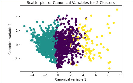
Cluster with green dots has low cluster variance somewhat, cluster with purple dots is also packed well enough, with some variance exists.

cluster with yellow dots isn't well separated from purple and Somewhat from cluster with purple , but it is much more spread on the plot

cluster with yellow it is much more spread on the plot, showing high variance in the plot. data is well separated (clusters overlap is not significant) k=>4 is a suitable number for current situation.

Cluster 0, had the highest Likelihood to be affected by Baseline value.

Cluster 3, includes fetals with higher likelihood of affected by Uterine contractions, Light decelerations, Severe decelerations,,Prolongued decelerations, Abnormal short term variability., Mean value of short term variability, Histogram mode

compared to the other two clusters. It also has higher levels affected by Histogram mean, Histogram median, Histogram variance.

In order to validate the clusters, ANOVA analysis was conducted to test for significant differences between the clusters on fetal health. Results indicated significant differences between the clusters on GPA (F(2, 1485)= 420.2, p<.0001). The tukey test showed that clusters differ significantly within fetal health, although difference between cluster 2 and 3 is not significant.

CODE:

!pip install statsmodels

from pandas import Series, DataFrame

import pandas as pd

import numpy as np

import matplotlib.pylab as plt

from sklearn.model_selection import train_test_split

from sklearn import preprocessing

from sklearn.cluster import KMeans

from scipy.spatial.distance import cdist

from sklearn.decomposition import PCA

import statsmodels.formula.api as smf

import statsmodels.stats.multicomp as multi

%matplotlib inline

RND_STATE = 2226

!pip install pandas

!pip install numpy

!pip install matplotlib

!pip install statsmodels

data = pd.read_csv("fetal_health.csv")

data.columns = map(str.upper, data.columns)

data_clean = data.dropna()

AH_data = pd.read_csv("fetal_health.csv")

data_clean = AH_data.dropna()

cluster=data_clean[['baseline value','uterine_contractions','light_decelerations','severe_decelerations',

'prolongued_decelerations',

'abnormal_short_term_variability','mean_value_of_short_term_variability',

'histogram_mode','histogram_mean',

'histogram_median','histogram_variance']]

cluster.describe()

clustervar=cluster.copy()

clustervar['baseline value']=preprocessing.scale(clustervar['baseline value'].astype('float64'))

clustervar['uterine_contractions']=preprocessing.scale(clustervar['uterine_contractions'].astype('float64'))

clustervar['light_decelerations']=preprocessing.scale(clustervar['light_decelerations'].astype('float64'))

clustervar['severe_decelerations']=preprocessing.scale(clustervar['severe_decelerations'].astype('float64'))

clustervar['prolongued_decelerations']=preprocessing.scale(clustervar['prolongued_decelerations'].astype('float64'))

clustervar['abnormal_short_term_variability']=preprocessing.scale(clustervar['abnormal_short_term_variability'].astype('float64'))

clustervar['mean_value_of_short_term_variability']=preprocessing.scale(clustervar['mean_value_of_short_term_variability'].astype('float64'))

clustervar['histogram_mode']=preprocessing.scale(clustervar['histogram_mode'].astype('float64'))

clustervar['histogram_mean']=preprocessing.scale(clustervar['histogram_mean'].astype('float64'))

clustervar['histogram_median']=preprocessing.scale(clustervar['histogram_median'].astype('float64'))

clustervar['histogram_variance']=preprocessing.scale(clustervar['histogram_variance'].astype('float64'))

clus_train, clus_test = train_test_split(clustervar, test_size=0.3, random_state=RND_STATE)

!pip install cluster

clusters=range(1,10)

meandist=[]

for k in clusters:

model=KMeans(n_clusters=k)

model.fit(clus_train)

clusassign=model.predict(clus_train)

meandist.append(sum(np.min(cdist(clus_train, model.cluster_centers_, 'euclidean'), axis=1))

/ clus_train.shape[0])

!pip install statsmodels

!pip install matplotlib

!pip install scipy

plt.plot(clusters, meandist)

plt.xlabel('Number of clusters')

plt.ylabel('Average distance')

plt.title('Selecting k with the Elbow Method')

plt.show()

model3=KMeans(n_clusters=3)

model3.fit(clus_train)

clusassign=model3.predict(clus_train)

pca_2 = PCA(2)

plot_columns = pca_2.fit_transform(clus_train)

plt.scatter(x=plot_columns[:,0], y=plot_columns[:,1], c=model3.labels_,)

plt.xlabel('Canonical variable 1')

plt.ylabel('Canonical variable 2')

plt.title('Scatterplot of Canonical Variables for 3 Clusters')

plt.show()

clus_train.reset_index(level=0, inplace=True)

cluslist=list(clus_train['index'])

labels=list(model3.labels_)

newlist=dict(zip(cluslist, labels))

newclus=DataFrame.from_dict(newlist, orient='index')

newclus.columns = ['cluster']

newclus.describe()

newclus.reset_index(level=0, inplace=True)

merged_train=pd.merge(clus_train, newclus, on='index')

merged_train.head(n=100)

merged_train.cluster.value_counts()

clustergrp = merged_train.groupby('cluster').mean()

print ("Clustering variable means by cluster")

print(clustergrp)

gpa_data=data_clean['fetal_health']

gpa_train, gpa_test = train_test_split(gpa_data, test_size=.3, random_state=RND_STATE)

gpa_train1=pd.DataFrame(gpa_train)

gpa_train1.reset_index(level=0, inplace=True)

merged_train_all=pd.merge(gpa_train1, merged_train, on='index')

sub1 = merged_train_all[['fetal_health', 'cluster']].dropna()

gpamod = smf.ols(formula='fetal_health ~ C(cluster)', data=sub1).fit()

print (gpamod.summary())

print ('means for fetal health by cluster')

m1= sub1.groupby('cluster').mean()

print (m1)

print ('standard deviations for fetal health by cluster')

m2= sub1.groupby('cluster').std()

print (m2)

mc1 = multi.MultiComparison(sub1['fetal_health'], sub1['cluster'])

res1 = mc1.tukeyhsd()

print(res1.summary())

[ghaida-2525]

HW.3 : Lasso Regression

At this HW. I have implemented lasso regression to predict Fetal Health on a list of explanatory variables. This time I’ve also selected all variables, that exist in given dataset. (baseline value, accelerations, fetal movement, uterine contractions, light decelerations, severe decelerations, prolongued decelerations, etc). All of them were used to build final model to predict the dependent variable – fetal_health .

In order to fit the Lasso Regression model, which helps to improve overall model quality and removes unimportant variables by adding an additional coefficient – alpha to each explanatory variable, I had to perform some preprocessing on data. In addiction to usual procedure of incomplete data removal, I’ve also added scaling to all of variables in order to lead it to one dimension.

In order to test final model I’ve split data into two sets – train (70%) and test(30%) to train and test Lasso Regression model respectively. Moreover, to reduce the influence of data imbalance I’ve added cv parameter (cv=10, default is 3) in order to specify the number of folds in a Stratified KFold, which helps to solve this problem. Change in the validation mean square error at each step:

in[19]: pred_train, pred_test, tar_train, tar_test = train_test_split(predictors, target, test_size=.3, random_state=RND_STATE)

Applying the Lasso Regression to the data assigns a Regression Coefficient to each predictor. Predictors with a Regression Coefficient of zero were eliminated,18 were retained.

{'baseline value': 0.18743121710692548 'accelerations': -0.012420438629578371, 'fetal_movement': -0.02678008761229712, 'uterine_contractions': -0.08881958546068254, 'light_decelerations': -0.025262653640074875, 'severe_decelerations': 0.0362727278281784, 'prolongued_decelerations': 0.20629467915907235, 'mean_value_of_short_term_variability': -0.034597706276368205, 'percentage_of_time_with_abnormal_long_term_variability': 0.2430909703179747, 'mean_value_of_long_term_variability': 0.0, 'histogram_width': 0.0, 'histogram_min': 0.08839831243779736, 'histogram_max': 0.05884828569739267, 'histogram_number_of_peaks': 0.0, 'histogram_number_of_zeroes': 0.0009254817992133355, 'histogram_mode': -0.10936885075312966, 'histogram_mean': -0.19033727038108944, 'histogram_median': 0.0, 'histogram_variance': 0.0865905038625272, 'histogram_tendency': 0.045210673662552284}

As seen, there 4 variables –mean value of long term variability, histogram width,histogram number of peaks, histogram median were removed by algorithm. It can be explained with the fact that Lasso Regression removes correlating variables from dataset.

The MSE for the training data stood at 0.1558 while it was 0.1716 for the test data.

IN[26] : train_error = mean_squared_error(tar_train, model.predict(pred_train))

test_error = mean_squared_error(tar_test, model.predict(pred_test))

print('training data MSE', train_error)

print('test data MSE', test_error)

training data MSE 0.1558480179256629 test data MSE 0.17166571196183492

Regression Coefficients Progression for Lasso Paths:

CODE:

import pandas as pd

import numpy as np

import matplotlib.pylab as plt

from sklearn.model_selection import train_test_split

from sklearn.linear_model import LassoLarsCV

from sklearn import preprocessing

from sklearn.metrics import mean_squared_error

pd.options.mode.chained_assignment = None

%matplotlib inline

RND_STATE = 2226

data = pd.read_csv("fetal_health.csv") data.columns = map(str.upper, data.columns) data.describe()

data_clean = data.dropna()

AH_data = pd.read_csv("fetal_health.csv")

data_clean = AH_data.dropna()

predvar = data_clean[['baseline value','accelerations','fetal_movement','uterine_contractions','light_decelerations','severe_decelerations','prolongued_decelerations','mean_value_of_short_term_variability', 'percentage_of_time_with_abnormal_long_term_variability','mean_value_of_long_term_variability','histogram_width','histogram_min','histogram_max','histogram_number_of_peaks','histogram_number_of_zeroes','histogram_mode','histogram_mean','histogram_median','histogram_variance','histogram_tendency']] target = data_clean.fetal_health

recode = {1:1, 2:0} data_clean['baseline value'] = data_clean['baseline value'].map(recode)

predictors=predvar.copy()

predictors['baseline value']=preprocessing.scale(predictors['baseline value'].astype('float64'))

predictors['accelerations']=preprocessing.scale(predictors['accelerations'].astype('float64'))

predictors['uterine_contractions']=preprocessing.scale(predictors['uterine_contractions'].astype('float64'))

predictors['light_decelerations']=preprocessing.scale(predictors['light_decelerations'].astype('float64'))

predictors['severe_decelerations']=preprocessing.scale(predictors['severe_decelerations'].astype('float64'))

predictors['prolongued_decelerations']=preprocessing.scale(predictors['prolongued_decelerations'].astype('float64'))

predictors['mean_value_of_short_term_variability']=preprocessing.scale(predictors['mean_value_of_short_term_variability'].astype('float64'))

predictors['percentage_of_time_with_abnormal_long_term_variability']=preprocessing.scale(predictors['percentage_of_time_with_abnormal_long_term_variability'].astype('float64'))

predictors['mean_value_of_long_term_variability']=preprocessing.scale(predictors['mean_value_of_long_term_variability'].astype('float64'))

predictors['histogram_width']=preprocessing.scale(predictors['histogram_width'].astype('float64'))

predictors['histogram_min']=preprocessing.scale(predictors['histogram_min'].astype('float64'))

predictors['histogram_max']=preprocessing.scale(predictors['histogram_max'].astype('float64'))

predictors['histogram_number_of_peaks']=preprocessing.scale(predictors['histogram_number_of_peaks'].astype('float64'))

predictors['histogram_number_of_zeroes']=preprocessing.scale(predictors['histogram_number_of_zeroes'].astype('float64'))

predictors['histogram_mode']=preprocessing.scale(predictors['histogram_mode'].astype('float64'))

predictors['histogram_mean']=preprocessing.scale(predictors['histogram_mean'].astype('float64'))

predictors['histogram_median']=preprocessing.scale(predictors['histogram_median'].astype('float64'))

predictors['histogram_variance']=preprocessing.scale(predictors['histogram_variance'].astype('float64'))

predictors['histogram_tendency']=preprocessing.scale(predictors['histogram_tendency'].astype('float64'))

pred_train, pred_test, tar_train, tar_test = train_test_split(predictors, target, test_size=.3, random_state=RND_STATE)

model = LassoLarsCV(cv=10, precompute=False).fit(pred_train,tar_train)

dict(zip(predictors.columns, model.coef_))

m_log_alphas = -np.log10(model.alphas_)

ax = plt.gca()

plt.plot(m_log_alphas, model.coef_path_.T)

plt.axvline(-np.log10(model.alpha_), linestyle='--', color='k',

label='alpha CV')

plt.ylabel('Regression Coefficients')

plt.xlabel('-log(alpha)')

plt.title('Regression Coefficients Progression for Lasso Paths')

m_log_alphascv = -np.log10(model.cv_alphas_)

plt.figure()

plt.plot(m_log_alphascv, model.mse_path_, ':')

plt.plot(m_log_alphascv, model.mse_path_.mean(axis=-1), 'k',

label='Average across the folds', linewidth=2)

plt.axvline(-np.log10(model.alpha_), linestyle='--', color='k',

label='alpha CV')

plt.legend()

plt.xlabel('-log(alpha)')

plt.ylabel('Mean squared error')

plt.title('Mean squared error on each fold')

train_error = mean_squared_error(tar_train, model.predict(pred_train))

test_error = mean_squared_error(tar_test, model.predict(pred_test))

print('training data MSE', train_error)

print('test data MSE', test_error)

rsquared_train=model.score(pred_train,tar_train)

rsquared_test=model.score(pred_test,tar_test)

print('training data R-square', rsquared_train)

print('test data R-square', rsquared_test)

[ghaida-2525]

Fetal Health Classification(Assignment2-Running a Random Forest)

Task:

Run a Random Forest.

You will need to perform a random forest analysis to evaluate the importance of a series of explanatory variables in predicting a binary, categorical response variable.

Solution:

In assignment No. 1, we chose four variables, which are Fetal movement ,Uterine contractions ,Histogram number of peaks and Histogram number of zeros to study the extent of their impact on the health of the fetus. In this assignment, we wrote a code that makes a random comparison between all the factors in the datasets that we applied in the first assignment. We obtained completely different results from what we obtained in the first assignment. The factors that are considered indicators of the health of the fetus here were other than those we chose in the previous assignment. As for the accuracy that we obtained here, it was greatly excellent than it was in the previous assignment, as we got here an accuracy of 93.5%, but in the previous assignment it was 74%.

Reading data from file

To show the frame of datasets:

Apply the Random Forest in Python:

Split into train test datasets

Split into training and testing sets

predictors = data_clean[['baseline value','accelerations','fetal_movement', 'uterine_contractions', 'light_decelerations', 'severe_decelerations', 'prolongued_decelerations',

'abnormal_short_term_variability', 'mean_value_of_short_term_variability', 'percentage_of_time_with_abnormal_long_term_variability','mean_value_of_long_term_variability','histogram_width','histogram_min','histogram_max','histogram_number_of_peaks','histogram_number_of_zeroes','histogram_mode',

'histogram_mean',

'histogram_median','histogram_variance', 'histogram_tendency']]

targets = data_clean.fetal_health

Apply train_test_split.

For example, you can set the test size to 0.4, and therefore the model testing will be based on 40% of the dataset, while the model training will be based on 60% of the dataset:

pred_train, pred_test, tar_train, tar_test = train_test_split(predictors, targets, test_size=.4, random_state=RND_STATE)

Build a Random Forest Classifier

Fitting RandomForestClassifier

Apply the Random Forest as follows:

classifier = RandomForestClassifier(n_estimators=22, random_state=RND_STATE)

classifier = classifier.fit(pred_train, tar_train)

predictions = classifier.predict(pred_test)

print the Accuracy

print(confusion_matrix(tar_test, predictions))

print()

print("Accuracy: ", accuracy_score(tar_test, predictions))

The output

Confusion matrix:

[[642 10 4]

[ 28 94 5]

[ 3 5 60]]

Accuracy: 0.9353701527614571

Final model looked excellent on test data and showed accuracy level at 93.5%!

Find important features with Random Forest model

important_features = pd.Series(data=classifier.feature_importances_,index=predictors.columns) important_features.sort_values(ascending=False,inplace=True)

After fitting the model it occurred that these factors influence final variable with different level of importance. So, I’ve calculated and sorted descending these factors into a feature importance list:

abnormal_short_term_variability 0.151485

percentage_of_time_with_abnormal_long_term_variability 0.118127

mean_value_of_short_term_variability 0.090103

histogram_mean 0.080043

prolongued_decelerations 0.076003

histogram_median 0.065495

histogram_mode 0.054925

accelerations 0.044466

uterine_contractions 0.044239

baseline value 0.042262

mean_value_of_long_term_variability 0.037475

histogram_variance 0.034731

histogram_min 0.034260

histogram_width 0.033916

histogram_max 0.028461

histogram_number_of_peaks 0.025365

fetal_movement 0.018233

light_decelerations 0.008666

histogram_number_of_zeroes 0.006063

histogram_tendency 0.005682

severe_decelerations 0.000000

dtype: float64

we see that the more factors that influnces the Fetal health

are:

abnormal_short_term_variability

percentage_of_time_with_abnormal_long_term_variability

mean_value_of_short_term_variability

histogram_mean

prolongued_decelerations

histogram_median

tested how number of trees in random forest influences on final model accuracy. So results can be presented in this plot:

As it shows, even one tree is able to show accuracy at a excellent level. So, this data can be described even with one tree. But, on the other hand, it is clear, that after adding some more trees (>7) final accuracy increases a bit, making model able to predict data in a better way.

Python code:

import pandas as pd

import numpy as np

import matplotlib.pylab as plt

from sklearn.model_selection import train_test_split

from sklearn.ensemble import RandomForestClassifier

from sklearn.ensemble import ExtraTreesClassifier

from sklearn.metrics import confusion_matrix

from sklearn.metrics import accuracy_score

%matplotlib inline

RND_STATE = 2226

AH_data = pd.read_csv("fetal_health.csv")

data_clean = AH_data.dropna()

data_clean.dtypes

data_clean.describe()

predictors = data_clean[['baseline value','accelerations','fetal_movement', 'uterine_contractions', 'light_decelerations', 'severe_decelerations', 'prolongued_decelerations',

'abnormal_short_term_variability', 'mean_value_of_short_term_variability', 'percentage_of_time_with_abnormal_long_term_variability','mean_value_of_long_term_variability','histogram_width','histogram_min','histogram_max','histogram_number_of_peaks','histogram_number_of_zeroes','histogram_mode',

'histogram_mean',

'histogram_median','histogram_variance', 'histogram_tendency']]

targets = data_clean.fetal_health

pred_train, pred_test, tar_train, tar_test = train_test_split(predictors, targets, test_size=.4, random_state=RND_STATE)

print("Predict train shape: ", pred_train.shape)

print("Predict test shape: ", pred_test.shape)

print("Target train shape: ", tar_train.shape)

print("Target test shape: ", tar_test.shape)

classifier = RandomForestClassifier(n_estimators=22, random_state=RND_STATE)

classifier = classifier.fit(pred_train, tar_train)

predictions = classifier.predict(pred_test)

print("Confusion matrix:")

print(confusion_matrix(tar_test, predictions))

print()

print("Accuracy: ", accuracy_score(tar_test, predictions))

important_features = pd.Series(data=classifier.feature_importances_,index=predictors.columns)

important_features.sort_values(ascending=False,inplace=True)

important_features

model = ExtraTreesClassifier(random_state=RND_STATE)

model.fit(pred_train, tar_train)

print(model.feature_importances_)

trees = range(22)

accuracy = np.zeros(22)

for idx in range(len(trees)):

classifier = RandomForestClassifier(n_estimators=idx + 1, random_state=RND_STATE)

classifier = classifier.fit(pred_train, tar_train)

predictions = classifier.predict(pred_test)

accuracy[idx] = accuracy_score(tar_test, predictions)

plt.cla()

plt.plot(trees, accuracy)

plt.show()

[ghaida-2525]

Fetal Health Classification (Decision Trees Assigment 1)

Task:

This week’s assignment involves decision trees, and more specifically, classification trees. Decision trees are predictive models that allow for a data driven exploration of nonlinear relationships and interactions among many explanatory variables in predicting a response or target variable. When the response variable is categorical (two levels), the model is a called a classification tree. Explanatory variables can be either quantitative, categorical or both. Decision trees create segmentations or subgroups in the data, by applying a series of simple rules or criteria over and over again which choose variable constellations that best predict the response (i.e. target) variable.

Run a Classification Tree.

You will need to perform a decision tree analysis to test nonlinear relationships among a series of explanatory variables and a binary, categorical response variable.

Generated decision tree :

                                     OPEN IMAGE

2126 measurements extracted from cardiotocograms and classified by expert obstetricians.

Decision tree analysis was performed to test nonlinear relationships among a series of explanatory variables and a binary, categorical response variable. All possible separations (categorical) or cut points (quantitative) are tested.

My decision tree uses these variables to predict output variable (fetal_health) – whether fetal health is good or no:

Fetal movement (fetal_movement=flMO).

Uterine contractions (uterin_contractions=Utrin).

Histogram number of peaks (histomgram_number_of_peaks=Peak).

Histogram number of zeros ( histomgram_number_of_ zeros=Zero).

After fitting the tree, I’ve tested it on test dataset and got accuracy = 0.74. This is a good result for a model, which is based only on four explaining variables.

From decision tree we can observe:

Uterine contractions are the  most important factor to determine if the fetal is in a good or no.

When Fetal movement is large value it means that the fetal is in good       state.

When  Histogram number of peaks are high  mean that fetal is in good condition

Formatted Source code (and output)

!pip install pydotplus

import pandas as pd import sklearn.metrics from numpy.lib.format import magic from sklearn.model_selection import train_test_split from sklearn.tree import DecisionTreeClassifier from sklearn import tree from io import StringIO from IPython.display import Image import pydotplus RND_STATE =2226

AH_data = pd.read_csv("fetal_health.csv") data_clean = AH_data.dropna() data_clean.dtypes  data_clean.describe()

predictors = data_clean[['fetal_movement','uterine_contractions', 'histogram_number_of_peaks', 'histogram_number_of_zeroes']]

targets = data_clean.fetal_health

pred_train, pred_test, tar_train, tar_test = train_test_split(predictors, targets, test_size=0.3)

classifier=DecisionTreeClassifier(random_state=RND_STATE)

classifier=classifier.fit(pred_train, tar_train) predictions=classifier.predict(pred_test)

print("Confusion matrix:\n", sklearn.metrics.confusion_matrix(tar_test,predictions)) print("Accuracy: ",sklearn.metrics.accuracy_score(tar_test, predictions))

out = StringIO() tree.export_graphviz(classifier, out_file=out, feature_names=["flMo", "Utrin", "Peak","Zero"],proportion=True, filled=True, max_depth=4) graph=pydotplus.graph_from_dot_data(out.getvalue()) img = Image(data=graph.create_png()) img

with open("utput" + ".png", "wb") as f: f.write(img.data)

[ghaida-2525]

Data science