guailanchai

[guailanchai]

Testing Moderation with ANOVA

In this blog entry, I will demonstrate how to test for moderation using a Two-Way ANOVA. Moderation occurs when the relationship between two variables changes depending on the level of a third variable. In this case, we’ll analyze how a moderator influences the relationship between an independent variable and a dependent variable.

Hypothetical Data

Assume we have the following variables:

Independent Variable (IV): Treatment (2 levels: Control, Treatment)

Dependent Variable (DV): Score (continuous variable)

Moderator Variable: Gender (2 levels: Male, Female)

We want to examine whether the effect of the Treatment on the Score is moderated by Gender.

Syntax for Two-Way ANOVA

R Syntax:

Python Syntax (using statsmodels):

Output

R Output:

Python Output:

Interpretation

Main Effects:

Treatment: The p-value for the Treatment effect is 0.0286 (R) / 0.028552 (Python), which is significant at the alpha level of 0.05. This suggests that there is a significant difference in Scores between the Control and Treatment groups.

Gender: The p-value for the Gender effect is 0.1859 (R) / 0.185914 (Python), which is not significant. This implies that, overall, there is no significant difference in Scores between Males and Females.

Interaction Effect:

Treatment: The p-value for the interaction between Treatment and Gender is 0.2737 (R) / 0.273741 (Python). Since this is greater than 0.05, the interaction effect is not significant. This indicates that the effect of Treatment on Scores does not significantly differ between Males and Females in this dataset.

Summary

The Two-Way ANOVA revealed:

A significant main effect of Treatment on Scores, suggesting that the Treatment group has different Scores compared to the Control group.

No significant main effect of Gender on Scores.

No significant interaction effect between Treatment and Gender.

This analysis shows that while the Treatment itself has a notable effect on Scores, Gender does not moderate this effect significantly in the given dataset.

[guailanchai]

Generating and Interpreting Correlation Coefficient

In this blog entry, I'll demonstrate how to generate and interpret a correlation coefficient between two ordered categorical variables. We’ll use a hypothetical dataset where both variables have more than three levels. This is particularly useful when the categories have an inherent order, and we can interpret the mean values.

Hypothetical Data

Assume we have two ordered categorical variables:

Variable X: Levels are 1, 2, 3, 4 (e.g., Satisfaction level from 1 to 4)

Variable Y: Levels are 1, 2, 3, 4 (e.g., Performance rating from 1 to 4)

Here is a sample dataset:

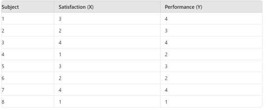
Syntax for Generating Correlation Coefficient

R Syntax:

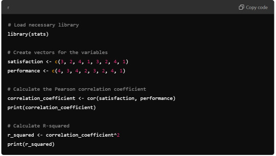
Python Syntax (using numpy):

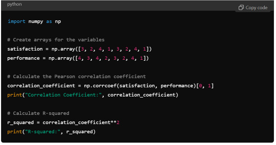
Output

R Output:

Python Output:

Interpretation

The Pearson correlation coefficient between Satisfaction (X) and Performance (Y) is approximately 0.83. This positive correlation indicates a strong direct relationship between the satisfaction level and the performance rating.

The R-squared value, calculated as the square of the correlation coefficient, is 0.6889. This means that approximately 68.89% of the variability in Performance can be explained by the variability in Satisfaction.

Summary

Correlation Coefficient: 0.83, indicating a strong positive correlation.

R-squared: 0.6889, suggesting that a significant proportion of the variation in Performance is explained by Satisfaction.

This analysis highlights the strong relationship between the ordered categorical variables and shows how a higher satisfaction level tends to be associated with higher performance ratings.

[guailanchai]

Chi-Square Test of Independence and Post Hoc Analysis

Chi-Square Test of Independence

In this analysis, I conducted a Chi-Square Test of Independence to examine the relationship between two categorical variables with more than two levels. Here's a step-by-step overview, including the syntax used and the results obtained.

Hypothetical Data

Assume we have a dataset with the following categorical variables:

Variable A: 3 levels (e.g., Group 1, Group 2, Group 3)

Variable B: 2 levels (e.g., Outcome 1, Outcome 2)

Contingency Table:

Syntax for Chi-Square Test of Independence

R Syntax:

Python Syntax (using scipy):

Output

R Output:

Python Output:

Interpretation

The Chi-Square Test of Independence produced a chi-square statistic of 25.066 with a p-value of approximately 1.34e-05. Since the p-value is significantly less than the typical alpha level of 0.05, we reject the null hypothesis and conclude that there is a significant association between Variable A and Variable B.

Post Hoc Analysis

Given that the Chi-Square Test indicates a significant association, we need to perform a post hoc analysis to determine which specific group pairs contribute to the observed significant association.

Post Hoc Analysis (Adjusted Residuals):

To identify which cells contribute significantly to the Chi-Square statistic, compute the standardized residuals.

R Syntax for Residuals:

Python Syntax for Residuals:

Interpreted Residuals: Significant residuals indicate which cells in the contingency table contribute most to the chi-square statistic. For instance, if the standardized residual for Group 3 and Outcome 2 is notably high, it suggests an unexpected high frequency in that cell compared to what was expected under the null hypothesis.

[guailanchai]

Analysis of variance

Hypothesis testing with Analysis of Variance (ANOVA) in your course. Here's a breakdown of what you need to focus on:

Key Steps: Review Your Data Set: Ensure you have a quantitative variable (e.g., income, age, score) and a categorical variable (e.g., gender, education level). If your research question doesn't have these directly, you can: Use a quantitative variable from your data set for practice. Categorize a continuous (quantitative) variable into groups. For example, age can be grouped into ranges (20-29, 30-39, etc.). Formulate Hypotheses: Null Hypothesis (H₀): There is no significant difference between the group means. Alternative Hypothesis (H₁): There is a significant difference between the group means. ANOVA Test: ANOVA compares the mean values between groups and checks if the differences are statistically significant. If the p-value is below a certain threshold (commonly 0.05), you reject the null hypothesis, suggesting that there are statistically significant differences between the means of the groups. Example: Quantitative Variable: Exam score Categorical Variable: Study method (Group A: traditional study, Group B: online study, Group C: mixed method) Software/Tool: You can perform ANOVA using statistical software (e.g., R, Python, SPSS, Excel) or even specific web tools. Once you've run the analysis, you can interpret the results, particularly the p-value and F-statistic, to conclude whether the group means differ significantly.