helloworldtester

[helloworldtester]

Time Series Analysis of S&P500

Load Packages

##Collecting the Data We will collect the S&P500 Stock Index monthly data starting from January 1, 1996 to April 1, 2019. This is an arbitrary range, you may choose a larger range if you prefer. We will get our data from Yahoo Finance, as it is a reliable source. From Yahoo Finance to get a csv file containing the Open, High, Low and Close price of S&P500.

##Reading the Data We will simply read the csv file we got from Yahoo Finance into R.

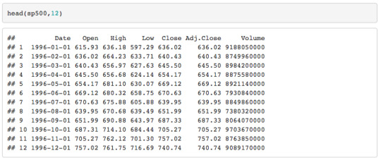
##Data Overview I’ve presented the first 12 rows as a visual.

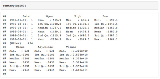
Here is the summary of the data.

##Exploratory Analysis We want to understand how the index is behaving overtime in order to model and forecast the S&P500. We want to ask questions like:

What’s the trend?

Is there cyclical/seasonal behaviour?

Is our seires stationary?

How does the ACF and PACF look?

Will our series be best represented by an autogressive (AR) model, a moving average (MA) model or an ARIMA model (cominbation of both AR and MA models)?

####Some Time Series Terminology Before we continue, I’d like to review some time series terminology.

What does it mean for a series to be stationary? We say a stochastic process ${Y_t}$ is stationary if

the expected value of $Y_t$ is constant overtime and

the autocovarice of $Y_{t, t-h}$ is equal to the autocovariance of $Y_{0,h}$.

What is ACF? ACF stands for autocorrelation function. Autocorrelation occurs when the error terms of a regression forecasting model are correlated. It’s used to detect the order of a moving average process.

What is PACF? PACF stands for partial autocorrelation function. It’s the correlation between $Y_t$ and $Y_{t-h}$. It’s used to detect the order of an autogressive process.

What is an autoregressive model? An autoregressive process is a regression on itself. It’s where the current value $Y_t$ is a linear combination of the past values plus an error term $e_t$ which incorporates everyting new in the series at time $t$ that is not explained in the past values. Here is an example of a third order autoregressive process: $Y_t = \phi_1Y_{t-1} + \phi_2Y_{t-2} + \phi_3Y_{t-3} + e_t$.

What is a moving average model? A moving average process is one whose current value $Y_t$ is a linear combination of the past error terms plus $e_t$ which incorporates everyting new in the series at time $t$ that is not explained in the past values. Here is an example of a second order moving average process: $Y_t = \theta_1e_{t-1} + \theta_2e_{t-2} + e_t$.

What is an ARMA model? An ARMA model is partly autoregressive and partly moving average. Here is an examle of ARMA(3,2) model: $Y_t = \phi_1Y_{t-1} + \phi_2Y_{t-2} + \phi_3Y_{t-3} + \theta_1e_{t-1} + \theta_2e_{t-2} + e_t$.

[helloworldtester]

Trading Options

Note to self: It’s all about the strike price and the expiry date. That’s it.

[helloworldtester]

Kawhi to Raptors, DeRozan to Spurs

How the fuck did this happen? Toronto, the 6ix, the “can never get a superstar”, has a superstar.

To all Raptors fan who think this was the worst decision made by the management, I humbly tell you, you’re dumb. Don’t get in your feelings. Relax.

Here’s the backstory. Kawhi Leonard, easily top 5 NBA player currently playing, has made it clear to everyone he wants to be with LeBron in LA. So much so that he walked away from a five year max contract worth $219 million dollars. Next year Kawhi becomes a free agent, which means he has the ability to choose where he wants to play. Essentially every team gives him a sales pitch for their Toyota Corolla ass team but instead he chooses a Lamborghini, drives to Hollywood and parks his car at the Lakers. Spurs and the great Popovich know that they’re no Lamborghini. So rather trade Kawhi now and get some assets in return than get nothing next year when he’s a free agent. Spurs called up every team and get rejected. No team wants to give up their assets for a player who’s only going to be a one year rental.

Is this seriously your argument? Raptors are dumb because they gave up DeRozan for Kawhi who might potentially be only a one year rental. Let’s be honest here, Raptors, at best, are just contenders for Eastern Conference Semi-Finals with DeRozan (and aging Lowry). They are NOT winning a championship with DeRozan. You know this, I know this. So let me ask you again, what good is it to keep DeRozan? I would rather grow a pair of balls, put all the chips on the table and gamble on Kawhi. Raptors desperately need a roster change. If Kawhi stays, we can attract better players and improve our roster. If Kawhi leaves, we start rebuilding our roster. It’s an inevitable change that needed to happen, so I’d rather take Kawhi in the process.

Welcome to the Raptors Kawhi. Ball out.

[helloworldtester]

Seamless Technology Is Underrated

This is a rather simple thought. I was driving down to class this morning when I remembered a conversation I had with my friend yesterday. He said he would love to get an Apple watch. He argued that it would drop his phone usage, save him time and let him focus on tasks at hand. Initially you may think this is silly, the aggregate time saved is probably less than 10 minutes in the entire day. The difference in time between looking at your Apple watch vs. pulling out your phone may just be 5 seconds or less.

I thought about it, I believe there is a bigger picture to be seen. Having an Apple watch on your wrist will make the information you receive via your mobile phone very seamless. Technology that is integrated in the backend of your life is worth having. This type of technology is underrated because it lacks your attention since it was designed so that the interaction between you and technology is natural and seamless.

Take for example keyless car entry. As long as the car keys are on you somewhere, when you open the door of your car it will unlock. You’re not actively thinking about finding your car keys to open your door as you approach your car. You’re touching yourself all over just to find that the car keys were in your back pocket the whole time. This seamless process of keyless car entry doesn’t break the flow you were in. As you are walking to your car having a conversation with either yourself or your friends, you carry that flow through the door into the car without any interruptions.

In this sense, having an Apple watch is quite similar. Having all your phone notifications available on your wrist will definitely increase your focus. The vibrations you feel from notifications on your wrist will stop you from checking your phone constantly in case you’ve missed something. Seeing information immediately on your wrist is definitely more natural and seamless than having to pull out your phone.

In conclusion, having thought about these technologies 5 minutes longer than usual I found an appreciation for them that I didn’t have before. Now I definitely want an Apple watch.

[helloworldtester]

Regression Analysis

I recently took one of my favourite courses in university: regression analysis. Since I really enjoyed this course, I decided to summarize the entire course in a few paragraphs and do it in such a way that a person from non-statistics/non-mathematics background can understand. So let’s get started.

What is regression analysis?

The first thing we learn in regression analysis is to develop a regression equation that models the relationship between a dependent variable, \( Y \) and multiple predictor variables \( x_1, x_2, x_3, \) etc. Once we have developed our model we would like to analyze it by performing regression diagnostics to check whether our model is valid or invalid.

So what the hell is a regression equation or a regression model? Well, to begin with, they are actually one and the same. A regression model just describes the relationship between a dependent variable \( Y \) and a predictor variable \( x \). I believe the best way to understand is to start with an example.

Example:

Suppose we want to model the relationship between \( Y \), salary in a particular industry and \( x \), the number of years of experience in that industry. To start, we plot \( Y \) vs. \( x \).

After a naive analysis of the plot suppose we come up with the following regression model: \( Y = \beta_0 + \beta_1x + e \). This regression model describes a linear relationship between \( Y \) and \( x \). This would result in the following regression line:

After graphing the regression line on to the plot we can visually see that our regression model is invalid. The plot seems to display quadratic behaviour and our model clearly does not account for that. Now after careful consideration we arrive at the following regression model: \( Y = \beta_0 + \beta_1x + \beta_2x^2 + e \). Again, let’s graph this regression model on to the plot and visually analyze the result.

It is clear that the latter regression model seems to describe the relationship between  \( Y \), salary in a particular industry and \( x \), the number of years of experience in that industry better than our first regression model.

This is essentially what regression analysis is. We develop a regression model to describe the relationship between a dependent variable, \( Y \) and the predictor variables \( x_1, x_2, x_3, \) etc. Once we have done that we perform regression diagnostics to check the validity of our model. If the results provide evidence against a valid model we must try to understand the problems within our model and try to correct our model.

Regression Diagnostics

As I’ve said earlier, once we develop our regression model we’d like to check if it is valid or not, for that we have regression diagnostics. Regression diagnostic is not just about visually analyzing the regression model to check if it’s a good fit or not, though it’s a good place to start, it is much more than that. The following is sort of a “check-list” of things we must analyze to determine the validity of our model.

1. The main tool that is used to validate our regression model is the standardized residual plots.

2. We must determine the leverage points within our data set.

3. We must determine whether outliers exist.

4. We must determine whether constant variance of errors in our model is reasonable and whether they are normally distributed.  

5. If the data is collected over time, we want to examine whether the data is correlated over time.

Standardized residual plots are arguably the most useful tool to determine the validity of the regression model. If there are any problems within steps 2 to 5, they would reflect in the residual plots. So to keep things simple, I will only talk about standardized residual plots. However, before I dive into that, it’s important to understand what residuals.

To understand what residuals are, we have to go back a few steps. It’s crucial that you understand that the regression model we come up with is an estimate of the actual model. We never really know what the true model is. Since we are working with an estimated model, it makes sense that there exists some “differences” between the actual and the estimated model. In statistics, we can these “differences” residuals. To get a visual, consider the graph below.

The solid linear line is our estimated regression model and the points on the graph are the actual values. Our estimated regression model is estimating the \( Y \) value to be roughly 3 when \( X = 2 \) but notice the actual value is roughly 7 when \( X = 2 \). So our residual, \( \hat{e}_3 \), is roughly equal to 4.

Now that we understand what residuals are, let’s talk about standardized residuals. The best way to think about standardized residuals is that they are just residuals which have been scaled down; since it’s usually easier to work with smaller numbers.

Now finally we can discuss standardized residual plots. These are just plots of standardized residuals vs. the predictor variables. Consider the regression model: \( Y = \beta_0 + \beta_1x_1 + \beta_2x_2 + \beta_3x_3 + \beta_4x_4 + e \), where \( Y \) is price, \(x_1\) is food rating, \(x_2\) is decor rating, \(x_3\) is service rating and \(x_4\) is the location of a restaurant, either to the east or west of a certain street. These predictor variables determines the price of the food at a restaurant. The following figure represents the standardized residual plots for this model.

When analyzing residual plots we check whether these plots are deterministic or not. In essence, we are checking to see if these plots display any patterns. If there are signs of pattern, we say the model is invalid. We would like the plots to be random. If they are random (non-deterministic) then we conclude that the regression model is valid. I’m not going to go into detail as to why that is, for that you’ll have to take the course.

Anyways, observing these plots we notice they are random, so we can conclude the regression model \( Y = \beta_0 + \beta_1x_1 + \beta_2x_2 + \beta_3x_3 + \beta_4x_4 + e \) is valid.

Alright we’re done. Semester’s over. Okay, so I’ve left out some topics. Some which are very exciting like variable selection, had to give a shoutout to that. However, this pretty much sums up regression analysis. This should provide a good overview into what you’re signing up for when taking this course.