iamcalledabhi-blog

[iamcalledabhi-blog]

k-means Cluster Analysis

Cluster analysis:

                           Cluster analysis or clustering is the task of grouping a set of objects in such a way that objects in the same group (called a cluster) are more similar (in some sense) to each other than to those in other groups (clusters). It is a main task of exploratory data mining, and a common technique for statistical data analysis, used in many fields, including pattern recognition, image analysis, information retrieval, bioinformatics, data compression, computer graphics and machine learning.

K-Means Clustering:                                   In this section, you will work with the Uber dataset, which contains data generated by Uber for the city on New York. Uber Technologies Inc. is a peer-to-peer ride sharing platform. Don’t worry if you don’t know too much about Uber, all you need to know is that the Uber platform connects you with (cab)drivers who can drive you to your destiny. The data is freely available on Kaggle. The dataset contains raw data on Uber pickups with information such as the date, time of the trip along with the longitude-latitude information.

New York city has five boroughs: Brooklyn, Queens, Manhattan, Bronx, and Staten Island. At the end of this mini-project, you will apply k-means clustering on the dataset to explore the dataset better and identify the different boroughs within New York. All along, you will also learn the various steps that you should take when working on a data science project in general.

Problem UnderstandingThere is a lot of information stored in the traffic flow of any city. This data when mined over location can provide information about the major attractions of the city, it can help us understand the various zones of the city such as residential areas, office/school zones, highways, etc. This can help governments and other institutes plan the city better and enforce suitable rules and regulations accordingly. For example, a different speed limit in school and residential zone than compared to highway zones.

The data when monitored over time can help us identify rush hours, holiday season, impact of weather, etc. This knowledge can be applied for better planning and traffic management. This can at a large, impact the efficiency of the city and can also help avoid disasters, or at least faster redirection of traffic flow after accidents.

However, this is all looking at the bigger problem. This tutorial will only concentrate on trying to solve the problem of identifying the five boroughs of New York city using k-means algorithm, so as to get a better understanding of the algorithms, all along learning to tackle a data science problem.

Understanding The DataYou only need to use the Uber data from 2014. You will find the following .csv files in the Kaggle link mentioned above:

uber-raw-data-apr14.csvuber-raw-data-may14.csvuber-raw-data-jun14.csvuber-raw-data-jul14.csvuber-raw-data-aug14.csvuber-raw-data-sep14.csvThis tutorial makes use of various libraries. Remember that when you work locally, you might have to install them. You can easily do so, using install.packages().

Let’s now load up the data:

# Load the .csv filesapr14 <- read.csv(“https://raw.githubusercontent.com/fivethirtyeight/uber-tlc-foil-response/master/uber-trip-data/uber-raw-data-apr14.csv”)may14 <- read.csv(“https://raw.githubusercontent.com/fivethirtyeight/uber-tlc-foil-response/master/uber-trip-data/uber-raw-data-may14.csv”)jun14 <- read.csv(“https://raw.githubusercontent.com/fivethirtyeight/uber-tlc-foil-response/master/uber-trip-data/uber-raw-data-jun14.csv”)jul14 <- read.csv(“https://raw.githubusercontent.com/fivethirtyeight/uber-tlc-foil-response/master/uber-trip-data/uber-raw-data-jul14.csv”)aug14 <- read.csv(“https://raw.githubusercontent.com/fivethirtyeight/uber-tlc-foil-response/master/uber-trip-data/uber-raw-data-aug14.csv”)sep14 <- read.csv(“https://raw.githubusercontent.com/fivethirtyeight/uber-tlc-foil-response/master/uber-trip-data/uber-raw-data-sep14.csv”)Let’s bind all the data files into one. For this, you can use the bind_rows() function under the dplyr library in R.

library(dplyr)data14 <- bind_rows(apr14, may14, jun14, jul14, aug14, sep14)So far, so good! Let’s get a summary of the data to get an idea of what you are dealing with.

summary(data14)  Date.Time Lat Lon Base         Length:4534327 Min. :39.66 Min. :-74.93 B02512: 205673   Class :character 1st Qu.:40.72 1st Qu.:-74.00 B02598:1393113   Mode :character Median :40.74 Median :-73.98 B02617:1458853                      Mean :40.74 Mean :-73.97 B02682:1212789                      3rd Qu.:40.76 3rd Qu.:-73.97 B02764: 263899                      Max. :42.12 Max. :-72.07                   The dataset contains the following columns:

Date.Time : the date and time of the Uber pickup;Lat: the latitude of the Uber pickup;Lon: the longitude of the Uber pickup;Base: the TLC base company code affiliated with the Uber pickup.Data PreparationThis step consists of cleaning and rearranging your data so that you can work on it more easily. It’s a good idea to first think of the sparsity of the dataset and check the amount of missing data.

# VIM library for using ‘aggr'library(VIM)

# 'aggr’ plots the amount of missing/imputed values in each columnaggr(data14)

As you can see, the dataset has no missing values. However, this might not always be the case with real datasets and you will have to decide how you want to deal with these values. Some popular methods include either deleting the particular row/column or replacing with a mean of the value.

You can see that the first column is Date.Time. To be able to use these values, you need to separate them. So let’s do that, you can use the lubridate library for this. Lubridate makes it simple for you to identify the order in which the year, month, and day appears in your dates and manipulate them.

library(lubridate)

# Separate or mutate the Date/Time columnsdata14$Date.Time <- mdy_hms(data14$Date.Time)data14$Year <- factor(year(data14$Date.Time))data14$Month <- factor(month(data14$Date.Time))data14$Day <- factor(day(data14$Date.Time))data14$Weekday <- factor(wday(data14$Date.Time))data14$Hour <- factor(hour(data14$Date.Time))data14$Minute <- factor(minute(data14$Date.Time))data14$Second <- factor(second(data14$Date.Time))#data14$date_timedata14$MonthLet’s check out the first few rows to see what our data looks like now….

head(data14, n=10)Date.Time Lat Lon Base Year Month Day Weekday Hour Minute Second2014-04-01 00:11:00 40.7690 -73.9549 B02512 2014 4 1 3 0 11 02014-04-01 00:17:00 40.7267 -74.0345 B02512 2014 4 1 3 0 17 02014-04-01 00:21:00 40.7316 -73.9873 B02512 2014 4 1 3 0 21 02014-04-01 00:28:00 40.7588 -73.9776 B02512 2014 4 1 3 0 28 02014-04-01 00:33:00 40.7594 -73.9722 B02512 2014 4 1 3 0 33 02014-04-01 00:33:00 40.7383 -74.0403 B02512 2014 4 1 3 0 33 02014-04-01 00:39:00 40.7223 -73.9887 B02512 2014 4 1 3 0 39 02014-04-01 00:45:00 40.7620 -73.9790 B02512 2014 4 1 3 0 45 02014-04-01 00:55:00 40.7524 -73.9960 B02512 2014 4 1 3 0 55 02014-04-01 01:01:00 40.7575 -73.9846 B02512 2014 4 1 3 1 1 0Awesome!

For this case study, this is the only data manipulation you will require for a good data understanding as well as to work with k-means clustering.

Now would be a good time to divide your data into training and test set. This is an important step in every data science project, it is done to train the model on the training set, determine the values of the parameters required and to finally test the model on the testing set. For example, when working with clustering algorithms, this division is done so that you can identify the parameters such as k, which is the number of clusters in k-means clustering. However, for this case study, you already know the number of clusters expected, which is 5 - the number of boroughs in NYC. Hence, you shall not be working the traditional way but rather, keep it primarily about learning about k-means clustering.

[iamcalledabhi-blog]

Lasso Regression Analysis

What is Lasso Regression?

Lasso regression is a type of linear regression that uses shrinkage . Shrinkage is where data values are shrunk towards a central point, like the mean. The lasso procedure encourages simple, sparse models (i.e. models with fewer parameters). This particular type of regression is well-suited for models showing high levels of muticollinearity or when you want to automate certain parts of model selection, like variable selection/parameter elimination.

Intro:This week I will try to explain the average daily volume of ethanol consumed per person in past year with a LASSO regression model.

DatasetNational Epidemiological Survey on Alcohol and Related Conditions (NESARC)CSV fileFile descriptionVariablesResponse:

ETOTLCA2 -> ETHANOL: average daily volume of ethanol consumed in past year (ounces).Explanatory:

AGE -> AGE: age (years).S1Q24LB -> WEIGHT: weight (pounds).NUMPERS -> HOUSE_PEOPLE: number of persons in household.S1Q4A -> MARRAIGE: age at first marriage (years).S1Q8D -> WORK: age when first worked full time, 30+ hours a week (years).S1Q12A -> INCOME: total household income in last 12 months (dolars).SEX -> MALE: gender (2 groups).S10Q1A63 -> CHANGE_MIND: change mind about things depending on people you’re with or what read or saw on tv (2 groups).All used variables are quantitative.

In [16]:%pylab inline

import numpy as npimport pandas as pd

from sklearn.cross_validation import train_test_splitimport sklearn.metricsfrom sklearn.linear_model import LassoLarsCV

#Visualizationimport matplotlib.pylab as pltimport seaborn as sns

pylab.rcParams[‘figure.figsize’] = (15, 8)Populating the interactive namespace from numpy and matplotlib

WARNING: pylab import has clobbered these variables: ['plt’]`%matplotlib` prevents importing * from pylab and numpy

DataIn [2]:# Load datadata = pd.read_csv(’../datasets/NESARC/nesarc_pds.csv’, usecols=['ETOTLCA2’,'AGE’,'S1Q24LB’,'NUMPERS’,'S1Q4A’,'S1Q8D’,'S1Q12A’,'SEX’,'S10Q1A63’])In [17]:# Custom dataframedf = pd.DataFrame()

# Response variabledf['ETHANOL’] = data['ETOTLCA2’].replace(’ ’,np.NaN).astype(float)

# Explanatory variablesdf['AGE’] = data['AGE’].replace(’ ’,np.NaN).replace('98’,np.NaN).astype(float)df['WEIGHT’] = data['S1Q24LB’].replace(’ ’,np.NaN).replace('999’,np.NaN).astype(float)df['HOUSE_PEOPLE’] = data['NUMPERS’].replace(’ ’,np.NaN).astype(float)df['MARRIAGE’] = data['S1Q4A’].replace(’ ’,np.NaN).replace('99’,np.NaN).astype(float)df['WORK’] = data['S1Q8D’].replace(’ ’,np.NaN).replace('99’,np.NaN).replace('0’,np.NaN).astype(float)df['INCOME’] = data['S1Q12A’].replace(’ ’,np.NaN).astype(float)df['MALE’] = data['SEX’].replace(’ ’,np.NaN).replace('2’,'0’).astype(float)df['CHANGE_MIND’] = data['S10Q1A63’].replace(’ ’,np.NaN).replace('9’,np.NaN).replace('2’,'0’).astype(float)

df = df.dropna()df.describe()Out[17]:ETHANOL AGE WEIGHT HOUSE_PEOPLE MARRIAGE WORK INCOME MALE CHANGE_MINDcount 15307.000000 15307.000000 15307.000000 15307.000000 15307.000000 15307.000000 15307.000000 15307.000000 15307.000000mean 0.490314 45.146338 174.669628 2.736199 23.537532 19.021297 62375.538642 0.503234 0.148559std 1.211545 13.486408 40.473162 1.422247 5.078884 4.496707 70392.218489 0.500006 0.355665min 0.000300 18.000000 78.000000 1.000000 14.000000 5.000000 24.000000 0.000000 0.00000025% 0.016800 35.000000 145.000000 2.000000 20.000000 17.000000 29999.000000 0.000000 0.00000050% 0.103700 43.000000 170.000000 2.000000 23.000000 18.000000 50000.000000 1.000000 0.00000075% 0.475450 54.000000 198.500000 4.000000 26.000000 21.000000 76000.000000 1.000000 0.000000max 29.676500 94.000000 450.000000 13.000000 63.000000 71.000000 3000000.000000 1.000000 1.000000In [4]:TARGET = 'ETHANOL'PREDICTORS = list(df.columns)PREDICTORS.remove(TARGET)

df_target = df[TARGET]df_predictors = pd.DataFrame()Standardize predictors0 Mean1 Standadrd deviationIn [5]:for predictor in PREDICTORS:    pred_data = df[predictor]     df_predictors[predictor] = (df[predictor] - df[predictor].mean()) / df[predictor].std()In [6]:df_predictors.describe()Out[6]:AGE WEIGHT HOUSE_PEOPLE MARRIAGE WORK INCOME MALE CHANGE_MINDcount 1.530700e+04 1.530700e+04 1.530700e+04 1.530700e+04 1.530700e+04 1.530700e+04 1.530700e+04 1.530700e+04mean -1.290461e-16 -5.756014e-17 -6.127369e-17 1.559694e-16 -8.541181e-17 -1.114067e-17 7.519953e-17 4.270591e-17std 1.000000e+00 1.000000e+00 1.000000e+00 1.000000e+00 1.000000e+00 1.000000e+00 1.000000e+00 1.000000e+00min -2.012866e+00 -2.388487e+00 -1.220744e+00 -1.877880e+00 -3.118126e+00 -8.857732e-01 -1.006456e+00 -4.176946e-0125% -7.523381e-01 -7.330692e-01 -5.176310e-01 -6.965176e-01 -4.495061e-01 -4.599449e-01 -1.006456e+00 -4.176946e-0150% -1.591483e-01 -1.153759e-01 -5.176310e-01 -1.058366e-01 -2.271212e-01 -1.758083e-01 9.935207e-01 -4.176946e-0175% 6.564878e-01 5.887944e-01 8.885945e-01 4.848444e-01 4.400337e-01 1.935507e-01 9.935207e-01 -4.176946e-01max 3.622437e+00 6.802789e+00 7.216609e+00 7.769910e+00 1.155928e+01 4.173223e+01 9.935207e-01 2.393937e+00Split: train, testIn [7]:train_target, test_target, train_predictors, test_predictors = train_test_split(df_target, df_predictors, test_size=0.3, random_state=42)

print('Samples train: {0}’.format(len(train_target)))print('Samples test: {0}’.format(len(test_target)))Samples train: 10714Samples test: 4593

ModelIn [8]:model1 = LassoLarsCV(cv=10,precompute=False)model1.fit(train_predictors, train_target)Out[8]:LassoLarsCV(copy_X=True, cv=10, eps=2.2204460492503131e-16,      fit_intercept=True, max_iter=500, max_n_alphas=1000, n_jobs=1,      normalize=True, positive=False, precompute=False, verbose=False)In [9]:print('Alpha parameter: {0}’.format(model1.alpha))Alpha parameter: 0.0

Regression coeficientsIn [10]:coefs = zip(df_predictors.columns,model1.coef_)coefs.sort(key=lambda x: abs(x[1]), reverse=True)print ’\n’.join( ’{0}: {1}’.format(var,coef) for var,coef in coefs)MALE: 0.25510029979HOUSE_PEOPLE: -0.0664057742071CHANGE_MIND: 0.0554624412918WEIGHT: -0.0550868686148WORK: -0.0437114356411AGE: -0.0349338129742MARRIAGE: -0.0195949134257INCOME: -0.0138293582608

PlotsIn [11]:# plot coefficient progressionm_log_alphas = -np.log10(model1.alphas_)ax = plt.gca()plt.plot(m_log_alphas, model1.coef_path_.T)plt.axvline(-np.log10(model1.alpha_), linestyle=’��’, color='k’,label='alpha CV’)plt.ylabel('Regression Coefficients’)plt.xlabel(’-log(alpha)’)plt.title('Regression Coefficients Progression for Lasso Paths’)Out[11]:<matplotlib.text.Text at 0x7fc86aa34550>

In [12]:# plot mean square error for each foldm_log_alphascv = -np.log10(model1.cv_alphas_)plt.figure()plt.plot(m_log_alphascv, model1.cv_mse_path_, ’:’)plt.plot(m_log_alphascv, model1.cv_mse_path_.mean(axis=-1), 'k’, label='Average across the folds’, linewidth=2)plt.axvline(-np.log10(model1.alpha_), linestyle=’–’, color='k’, label='alpha CV’)plt.legend()plt.xlabel(’-log(alpha)’)plt.ylabel('Mean squared error’)plt.title('Mean squared error on each fold’)Out[12]:<matplotlib.text.Text at 0x7fc86a8669d0>

MetricsIn [13]:# MSE from training and test dataprint ('MSE training: {0}’.format(sklearn.metrics.mean_squared_error(train_target, model1.predict(train_predictors))))print ('MSE testing: {0}’.format(sklearn.metrics.mean_squared_error(test_target, model1.predict(test_predictors))))MSE training: 1.51194970787MSE testing: 1.15947090575

In [14]:# R-square from training and test dataprint ('R-square training: {0}’.format(model1.score(train_predictors,train_target)))print ('R-square testing: {0}’.format(model1.score(test_predictors,test_target)))R-square training: 0.0396962849816R-square testing: 0.048380464543

SummaryIn this assignment, the LASSO regression hasn’t proved to be very valuable as the model can only explain a 4,8% of the variance (R-Squared value). It is surprising this value is higher in the test dataset than in the training one. It happens the same with the Mean Squared Error, it is lower in the testing dataset.

The prediction accuracy is pretty stable as the metric values are similar in training and testing datasets.

The most important variable to predict the alcohol ingest is MALE: 0.25510029979, followed by HOUSE_PEOPLE: -0.0664057742071 CHANGE_MIND: 0.0554624412918, WEIGHT: -0.0550868686148 and WORK: -0.0437114356411. Surprisingly, the income is not as relevant as the others but it is not discarded.

One bad thing about the results is getting an Alpha value of 0, this means no regularization has been done and an Ordinary Least Squares regression has been performed. This can be verified as no predictor has been discarded, every one has a coefficient bigger than one.

The LASSO regression is useful when there are few observations and a large number of predictors so it can be used for dimensionality reduction.

[iamcalledabhi-blog]

Running a Random Forest

Random Forest

Random Forests (RFs) are composed of multiple independent decision trees that are trained independently on a random subset of data.

The random forest is a classification algorithm consisting of many decisions trees. It uses bagging and feature randomness when building each individual tree to try to create an uncorrelated forest of trees whose prediction by committee is more accurate than that of any individual tree

During implementation of home work #2 I have fitted several classifiers, including RandomForestClassifier and ExtraTreesClassifier to predict binary response variable – TREG1 (whether person is a smoker or not).

All variables, that exist in dataset, like age, gender, race, alcohol use and others (see dataset) were used to build final model. After fitting the model it occurred that these factors influence final variable with different level of importance. So, I’ve calculated and sorted descending these factors into a feature importance list: marever1 0.096374 age 0.083599 DEVIANT1 0.080081 SCHCONN1 0.075221 GPA1 0.074775 DEP1 0.071728 FAMCONCT 0.067389 PARACTV 0.063784 ESTEEM1 0.057945 ALCPROBS1 0.057670 VIOL1 0.048614 ALCEVR1 0.043539 PARPRES 0.039425 WHITE 0.022146 cigavail 0.021671 BLACK 0.018512 BIO_SEX 0.014942 inhever1 0.012832 cocever1 0.012590 PASSIST 0.010221 EXPEL1 0.009777 HISPANIC 0.007991 NAMERICAN 0.005332 ASIAN 0.003844 So, there is no surprise in output here after HW1. Previous marijuana usage, age and school grades are still ones that influence the most. Final model looked well on test data and showed accuracy level at 83,4%! Also during this home work I’ve tested how number of trees in random forest influences on final model accuracy. So results can be presented in this plot: plot As it shows, even one tree is able to show accuracy at a good level. So, this data can be described even with one tree. But, on the other hand, it is clear, that after adding some more trees (>5) final accuracy increases a bit, making model able to predict data in a better way.

CODING :

import pandas as pd

import numpy as np

import matplotlib.pylab as plt

from sklearn.model_selection import train_test_split

from sklearn.ensemble import RandomForestClassifier

from sklearn.ensemble import ExtraTreesClassifier

from sklearn.metrics import confusion_matrix

from sklearn.metrics import accuracy_score

%matplotlib inline

RND_STATE = 55324

AH_data = pd.read_csv(“data/tree_addhealth.csv”)

data_clean = AH_data.dropna()

data_clean.dtypes

data_clean.describe()

predictors = data_clean[[‘BIO_SEX’, ‘HISPANIC’, ‘WHITE’, ‘BLACK’, ‘NAMERICAN’, ‘ASIAN’, ‘age’,

‘ALCEVR1’, ‘ALCPROBS1’, ‘marever1’, ‘cocever1’, ‘inhever1’, ‘cigavail’, ‘DEP1’, ‘ESTEEM1’,

‘VIOL1’,

‘PASSIST’, ‘DEVIANT1’, ‘SCHCONN1’, ‘GPA1’, ‘EXPEL1’, ‘FAMCONCT’, ‘PARACTV’, ‘PARPRES’]]

targets = data_clean.TREG1

pred_train, pred_test, tar_train, tar_test = train_test_split(predictors, targets, test_size=.4, random_state=RND_STATE)

print(“Predict train shape: “, pred_train.shape)

print(“Predict test shape: “, pred_test.shape)

print(“Target train shape: “, tar_train.shape)

print(“Target test shape: “, tar_test.shape)

classifier = RandomForestClassifier(n_estimators=25, random_state=RND_STATE)

classifier = classifier.fit(pred_train, tar_train)

predictions = classifier.predict(pred_test)

print(“Confusion matrix:”)

print(confusion_matrix(tar_test, predictions))

print()

print(“Accuracy: “, accuracy_score(tar_test, predictions))

important_features = pd.Series(data=classifier.feature_importances_,index=predictors.columns)

important_features.sort_values(ascending=False,inplace=True)

print(important_features)

model = ExtraTreesClassifier(random_state=RND_STATE)

model.fit(pred_train, tar_train)

print(model.feature_importances_)

trees = range(25)

accuracy = np.zeros(25)for idx in range(len(trees)):

classifier = RandomForestClassifier(n_estimators=idx + 1, random_state=RND_STATE)

classifier = classifier.fit(pred_train, tar_train)

predictions = classifier.predict(pred_test)

accuracy[idx] = accuracy_score(tar_test, predictions)

plt.cla()

plt.plot(trees, accuracy)

plt.show()

[iamcalledabhi-blog]

Decision Tree

Machine Learning(ML):

                                  Machine learning is an application of artificial intelligence (AI) that provides systems the ability to automatically learn and improve from experience without being explicitly programmed. Machine learning focuses on the development of computer programs that can access data and use it learn for themselves.It is the field of study that gives computers the capability to learn without being explicitly programmed. ML is one of the most exciting technologies that one would have ever come across. As it is evident from the name, it gives the computer that makes it more similar to humans: The ability to learn. Machine learning is actively being used today, perhaps in many more places than one would expect.

Classification Tree:

                                    Kaggle.com has a Titanic dataset in the ‘Getting started’ section along with some handy machine learning tutorials. I have been a member of kaggle for a year or so as I had to enter a competition as part of my first ever completed MOOC on Machine learning. Back then I had to learn R which seems very nice for machine learning but not much good for anything else. In the interim I have spent time learning some web development as part of a job requirement and Python because it seems a much better language for all purpose programming. I then enrolled in this course to learn about Machine Learning in Python and so now the circle closes as I get back to kaggle after a long break. My current kaggle ranking is 69,710th after hitting a high of 50,058th after my one and only competition. I intend using the next few lessons on this MOOC to begin pushing that higher.

The kaggle training set has 891 records with features as described below. For the purpose of this assignment I will see how a classification can predict survival using only Sex, Age and Passenger Class. I needed to create a categorical feature for sex which I called Gender (Female = 1, Male = 0) and I also split Age into three categories (Under 8 = 0, 8 - 16 = 1, over 16 = 2) simply to keep the picture of the tree nice and compact. Passenger class was naturally categorical with 1, 2 & 3 representing 1st, 2nd and 3rd class.

The performance of even this simple model was quite reasonable with around 80% accuracy and correctly predicting 294 of the 357 test cases. One can see from the training set that of 534 passengers, 348 were male but only 72 of those survived while out of 207 female passengers 135 survived. At least 134 of the 207 survivors were 1st class passengers. Apparantly the lifeboats were loaded on a women and children first basis but also they were often not filled leaving many passengers in the water around 2.5 hours after the accident. It is beleived that the high ratio of 1st class survivors is due to those cabins being on the upper decks of the ship.

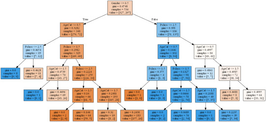
CODING:

# coding: utf-8

“’

Decision tree to predict survival on the TtTanic

”’

get_ipython().magic('matplotlib inline’)

from pandas import Series, DataFrame

import pandas as pd

import numpy as np

import os

import matplotlib.pylab as plt

from sklearn.cross_validation import train_test_split

from sklearn.tree import DecisionTreeClassifier

from sklearn.metrics import classification_report

import sklearn.metrics

titanic = pd.read_csv('train.csv’)

print(titanic.describe())

print(titanic.head(5))

print(titanic.info())

# simplify Age

def catAge (row):

 if row['Age’] <= 8 :

    return 0

 elif row['Age’] <= 16 :

    return 1

 elif row['Age’] <= 60 :

    return 2

 else:

    return 2

# create categorical varioble for sex 1 = female, 0 = male

titanic['Gender’] = titanic['Sex’].map( {'female’: 1, 'male’: 0} ).astype(int)

# create age categories either 1 = Adult or 0 = child

titanic['AgeCat’] = titanic.apply(lambda row:catAge(row), axis = 1)

print(titanic.dtypes)

# get a clean subset

sub = titanic[['PassengerId’, 'Gender’,'Pclass’, 'AgeCat’,'SibSp’, 'Survived’]].dropna()

sub['Gender’] = sub['Gender’].astype('category’)

sub['AgeCat’] = sub['AgeCat’].astype('category’)

sub['Pclass’] = sub['Pclass’].astype('category’)

print(sub.info())

# Split the data

predictors = sub[['Gender’,'Pclass’, 'AgeCat’,'SibSp’]]

targets = sub['Survived’]

pred_train, pred_test, tar_train, tar_test  =   train_test_split(predictors, targets, test_size=.4)

print(pred_train.shape, ’\n’,

pred_test.shape,’\n’,

tar_train.shape,’\n’,

tar_test.shape)

#Build model on training data

classifier=DecisionTreeClassifier()

classifier=classifier.fit(pred_train,tar_train)

predictions=classifier.predict(pred_test)

print(’\nConfusion Matrix’)

print(sklearn.metrics.confusion_matrix(tar_test,predictions))

print('Accuracy Score’)

print(sklearn.metrics.accuracy_score(tar_test, predictions))

#Displaying the decision tree

from sklearn import tree

#from StringIO import StringIO

from io import StringIO

#from StringIO import StringIO

from IPython.display import Image

out = StringIO()

tree.export_graphviz(classifier, out_file=out, feature_names = ['Gender’, 'Pclass’,'AgeCat’,'SibSp’],filled = True)

import pydotplus

graph=pydotplus.graph_from_dot_data(out.getvalue())

Image(graph.create_png())

# Split the data

predictors = sub[['Gender’,'Pclass’, 'AgeCat’]]

targets = sub['Survived’]

pred_train, pred_test, tar_train, tar_test  =   train_test_split(predictors, targets, test_size=.4)

print(pred_train.shape, ’\n’,

pred_test.shape,’\n’,

tar_train.shape,’\n’,

tar_test.shape)

#Build model on training data

classifier=DecisionTreeClassifier()

classifier=classifier.fit(pred_train,tar_train)

# Make prediction on the test data

predictions=classifier.predict(pred_test)

# Confusion Matrix

print('Confusion Matrix’)

print(sklearn.metrics.confusion_matrix(tar_test,predictions))

#Accuracy

print('Accuracy Score’)

print(sklearn.metrics.accuracy_score(tar_test, predictions))

# Show the tree

out = StringIO()

tree.export_graphviz(classifier, out_file=out, feature_names = ['Gender’,'Pclass’, 'AgeCat’],filled = True)

# Save tree as png file

graph=pydotplus.graph_from_dot_data(out.getvalue())

Image(graph.create_png())

print(pred_train.describe())

# Observe various features of the traning data

print(titanic.Gender.sum())

print(titanic.Gender.count())

print(titanic.Gender.sum()/titanic.Gender.count())

# Table of survival Vs Gender

pd.crosstab(titanic.Sex,titanic.Survived)