jane-doe-coursera-blog

[jane-doe-coursera-blog]

Course 4 - Week 3

A lasso regression analysis was conducted to identify a subset of variables from a pool of 17 categorical and quantitative predictor variables  that best predicted a quantitative response variable measuring a categorical variable that describes whether a person is alcoholic or not.

The possible explanatory variables included whether a family member is alcoholic, whether the individual is a retiree, employed full-time or unemployed, the age at first marriage, the race, the age at which the individuals had their first child and the number of children under 18.

Data were randomly split into a training set that included 70% of the observations (N=14,130) and a test set that included 30% of the observations (N=5992). The least angle regression algorithm with k=10 fold cross validation was used to estimate the lasso regression model in the training set, and the model was validated using the test set. The change in the cross validation average (mean) squared error at each step was used to identify the best subset of predictor variables.

Of the 17 predictor variables, 12 were retained in the selected model. The most significant predictors were whether a person is working full time (S1Q7A1) or is retired (S1Q7A9), followed by the sex and whether the person is white (S1Q1D5). S1Q7A1 (1=yes and 2=no) was positively related with alcoholism, indicating that not working full time increases the chance that a person is alcoholic. It is the other way around for S1Q7A9: Being retired increases the risk of being alcoholic as there was a negative association between the two variables. S1Q1D5 was positively associated with alcoholism, indicating that non-white races are more likely to affected by alcoholism. Another interesting finding is that women are more likely to be alcoholic than men as the variable sex () was positively associated with alcoholism. The 12 selected variables accounted for 10.4% of the variance in the alcoholism response variable.

[jane-doe-coursera-blog]

Course 4 - Week 4

I ran a random forest procedure tree for my binary categorical response variable “Alcoholic“. Because SAS tests for the occurrence of the lowest value the variable takes on, I coded Alcoholic=1 if the person is alcohol-dependent and Alcoholic=2 is the person is not. With this, the model event predicted is the presence of alcoholism and not its absence.

The possible explanatory variables included whether a family member is alcoholic, whether the individual is a retiree, employed full-time or unemployed, the age at first marriage, the race, the age at which the individuals had their first child and the number of children under 18.

The random variable set to be tested as splits consisted at each node of four variables each time. 100 trees were grown by the procedure and 60% of the sample data were used in the bagging process and thus used in growing the trees. The remaining 40% were used as test data. By default, there was no pruning.

The procedure read 43,093 observations and used all of them. The misclassification rate is 37.5% so that the forest correctly classified 62.5%. The fit statistics show that the out-of-bag misclassification rate decreases from 32.8% for a forest with a single tree to between 31.5% and 31.7% for a forest with 39 trees or more. From there it fluctuates around this level. The misclassification rate of the training sample is even reduced to 27.5%.

The most important predictors in terms of variable importance are employment status (S1Q7A1 = full time employed, S1Q7A9 = retiree, S1Q7A2 = part-time employed), race (S1Q1D5 = white, S1Q1D3 = black, S1Q1C = hispanic), gender and family history. These variables could be used in further analysis.

[jane-doe-coursera-blog]

Course 4 - Week 1

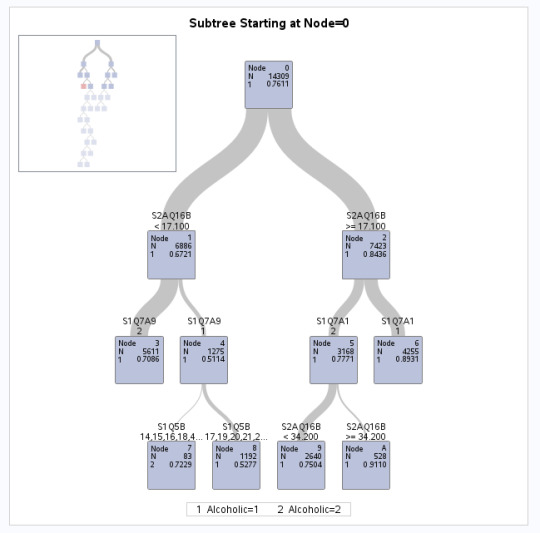
I built a decision tree for my binary categorical response variable “Alcoholic“. Because SAS tests for the occurrence of the lowest value the variable takes on, I coded Alcoholic=1 if the person is alcohol-dependent and Alcoholic=2 is the person is not. With this, the model event predicted is the presence of alcoholism and not its absence.

The output of the HPSPLIT procedure is presented above. We can see that the tree had 348 leaves before pruning and 15 leaves after pruning. There were 43,093 observations read from the data set and 14,309 thereof were used as these had valid data for the explanatory as well as the target variables.

The cost-complexity analysis shows the crossvalidated average standard error (ASE) for each number of leaves. The tree with 13 leaves has the lowest ASE. The final tree has splits for the age when a person first started drinking alcohol weekls (S2AQ16B) as a split node twice, whether the person is retired (S1Q7A9), the age at which the individuals had their first child (S1Q5B), whether they are employed full-time (S1Q7A1).

When we look at the confusion matrix, it becomes clear that the model correctly predicted 97% (error rate=0.03) of the Alcoholics, but only 13% (error rate=0.87) of the non-alcoholics. So we are more likely to correctly predict the presence of alcoholism rather than its absence.

There are some variables that are included in the variable importance training that were not selected as split nodes, such as age at first marriage, the race variables or drinking starting age. These are thus masked by other variables that were included as splits.

[jane-doe-coursera-blog]

Course 3 Week 4 Assignment

I ran a logistic regression on two binary variables, coded zero and one, respectively. My response variable was “Alcoholic” which takes on the value of one if a person reports to be addicted to alcohol and zero otherwise. Because of this, I needed to add the option “descending” to my logistic regression in order to measure the presence of alcoholism and not the absence of it. The explanatory variable is Family_History and takes on the value of one if the person reported that at least one of the family members suffers or previously suffered from alcoholism.

My hypothesis is that there is a certain family disposition to alcoholism. This means that I believe that as family members are alcoholic, an individual is more likely to be addicted to alcohol as well.

The results of the logistic regression are presented below.

It shows that the regression is significant at an alpha level of 0.0196 and the coefficient of family history is 0.0709. This regression has an odds ratio of 1.073. As this figure is greater than one, this means those individuals with a family history of alcoholism are 1.073 times more likely to be alcoholics themselves. The 95% confidence interval lies between 1.011 and 1.139.

As the confidence interval does not include 1 the relationship is statistically significant and reinforces my hypothesis that a person is more likely to become addicted to alcohol at some point in their life if they have relatives who suffer from alcohol dependence.

It would be possible that the family history is not really the driving factor behind an individual’s alcoholism, but that rather the family history of alcoholism influences the individual’s drinking starting age, which in return is the variable for explaining alcoholism. So I added another binary explanatory variable that takes on the value of zero if the individual started drinking before the age of 30 and one otherwise.

The results of that second logistic regression are also shown below. We can see that family history still has an odds ration greater than one with a statistically significant 95% confidence interval of 1.006 to 1.134 (p-value = 0.0309). In addition to that, drinking age group has an odds ratio smaller than one (0.896) with a 95% confidence interval of 0.838 to 0.957, which is also statistically significant (p-value = 0.0011). This means that there is no significant evidence of confounding between these two variables, but rather that they are both valid predictors of alcohol abuse as they remain statistically significant after controlling for the other variable, respectively.

[jane-doe-coursera-blog]

Course 3 Week 3 Assignment

My explanatory variables for my multiple linear regression model are family history of alcohol abuse, sex and the number of times a person drank in the last year. Family history was reported on a single-family member basis from spouses to children and parents and grand-parents. I used these variables to count the number of alcohol-dependent family members, as well as to create a single two-level categorical variable that takes the value of one if the individual has any alcohol-dependent family members and zero otherwise. The binary variables family_history and sex were coded so that one of the values is zero. The quantitative variables Drinks_per_day and Drinks_L12M were centered around zero by subtracting the mean.

My hypothesis is that the family history will have a positive association with drinks per day in that a person with a family history of alcohol abuse tends to drink more. The same is expected to hold true for the number of times a person drinks. Sex is included as a control variable only.

I then ran a multiple linear regression analysis with the number of drinks a person drinks per drinking day as response variable. The results are presented below. The best fit regression line would be

Drinks_per_day =0.211 + 0.572 * family_history – 0.215 * Drinks_L12M - 0.823 * sex.

There is thus a positive relationship between the family history and the number of times a person drank (Beta=0.572), the sex (Beta=-0.823) as well as the number of times a person drank in the past year (Beta=-0.215) after controlling for all the other variables. This relationship is statistically significant with a p-value <0.0001 but r-square is only 0.115 indicating that not too much of the variability in the drinks per day is explained by the three explanatory variables.

This shows that the hypothesis for family_history is supported by the results. However, the results are the opposite for the variable Drinks_L12M. While there is a statistically significant relationship, it is the opposite of what I initially expected. The beta coefficient of the variable sex indicates that females on average drink almost one drink less than males.

As you can see all the variables are statistically significant and there is no indication for confounding variables because all explanatory variables are statistically significant in individual regressions as well as in the multiple linear regression conducted.

Next, I also include a q-q plot. It becomes obvious that the residuals do not follow a straight line, particularly towards the lower and upper quantiles. This indicates that there may be other variables that influence the drinks per day of an individual that is not accounted for in the linear regression and that thus the model is not a really good fit.

The next plot I include is a plot showing the standardized residuals. We can see that there are quite a few outliers outside of three times the standard deviation, one extreme outlier above 40. This might indicate that these outliers strongly influence the model and that therefore the level of error in the model is not acceptable.

The last plot that I included is the outlier and leverage diagnostic. It shows that there are many outliers that have residuals greater than two, but it also shows that there are no leveraging observations, i.e. observations that strongly influence the model. This means that although there are outliers, they do not have a strong influence on the estimation of parameters.

Overall, we can conclude that model fit would need to be improved by including additional explanatory variables.

[jane-doe-coursera-blog]

Week 2 Assignment

My explanatory variable is family history of alcohol abuse. Family history was reported on a single-family member basis from spouses to children and parents and grand-parents. I used these variables to count the number of alcohol-dependent family members, as well as to create a single two-level categorical variable that takes the value of one if the individual has any alcohol-dependent family members and zero otherwise.

Because I have a binary categorical explanatory variable I present below the output of the frequency procedure that shows that it was successfully created with two levels, one of which is zero. My sample includes 14,431 individuals without alcohol-dependent family members and 11,781 individuals with a family history of alcohol abuse.

I then ran a linear regression analysis with the number of drinks a person drinks per drinking day as response variable. The results are also presented below. The best fit regression line would be y=2.306+0.508x. There is thus a positive relationship between the family history and the number of times a person drank (Beta=0.508). Thus, a person with a family history of alcohol abuse would on average drink 0.5 drinks more on a drinking day than one without a family history. This relationship is statistically significant with a p-value <0.0001 but r-square is only 0.011 indicating that very little of the variation of the number of drinks is explained by the family history.

[jane-doe-coursera-blog]

Week1-Measures

Measures

My response variables are concerned with the drinking behavior of the individuals. Because a substantial number of NESARC respondents were nondrinkers (either lifetime abstainers or former drinkers), NESARC included some screener questions to determine current drinking status. Only respondents who reported having at least 1 drink of any type of alcohol in the past year were considered to be current drinkers and were asked detailed questions about past-year alcohol consumption. For the NESARC, lifetime abstainers were those who never had 1 or more drinks in their life, and former drinkers were those who had at least 1 drink in their life, but not in the past year. Most of the tables in this manual are based on current drinkers only (see data manual on NESARC from NIH https://www.niaaa.nih.gov/). Because I am only interested in those who drank in their lifetime, I excluded lifetime abstainers in my analysis. Current drinking was evaluated through further questions, such as “How often did you drink any alcohol in the last 12 months?” with categories ranging from one time to every day or “How many drinks did you usually consume on days when you drank alcohol?”, a quantitative variable ranging from 1 to 98 drinks. My explanatory variable is family history of alcohol abuse. Family history was reported on a single-family member basis from spouses to children and parents and grand-parents. I used these variables to count the number of alcohol-dependent family members, as well as to create a single two-level categorical variable that takes the value of one if the individual has any alcohol-dependent family members and zero otherwise.

[jane-doe-coursera-blog]

Week1-Procedure

Procedure

The observational data was generated by a survey research study: Data were collected by trained U.S. Census Bureau Field Representatives during 2001–2002 through computer-assisted personal interviews (CAPI). One adult was selected for interview in each household, and interviews were conducted in respondents’ homes following informed consent procedures. The original purpose of the study was to provide a nationwide longitudinal survey of alcohol and drug use and associated psychiatric and medical comorbidities.

[jane-doe-coursera-blog]

Week1-Sample

Sample

The sample is from the first wave of the National Epidemiologic Survey on Alcohol and Related Conditions (NESARC), the largest nationwide longitudinal survey of alcohol and drug use and associated psychiatric and medical comorbidities. Participants (N=43,093) represented the civilian, non-institutionalized adult population of the United States, and included persons living in households, military personnel living off base, and persons residing in the following group quarters: boarding or rooming houses, non-transient hotels and motels, shelters, facilities for housing workers, college quarters, and group homes. The NESARC included over sampling of Blacks, Hispanics and young adults aged 18 to 24 years. The data analytic sample for this study included participants 18-25 years old who reported smoking at least 1 cigarette per day in the past 30 days (N=1,320).

[jane-doe-coursera-blog]

Week 4 Moderators

I tested a potential moderator between a categorical explanatory variable and a quantitative response variable. I tested whether the person’s drinking status acts as a moderator between the family history of alcoholism and the drinking starting age. The output is presented below.

It becomes obvious that the results are slightly different for those who are alcoholic: They started drinking on average at 20.4 years if they had no alcoholic family member and started drinking earlier at 18.5 years if they had a family history of alcoholism.

Compared to that, people who are not currently drinking started drinking earlier at 20.1 years if they had no previous history of alcoholism in the family and later at 18.8 years if they had alcoholic family members. So we can see that, while the current drinking status acts as a moderator between the two variables in that there is a much bigger gap in the drinking ages for those who are current drinkers, it does not change the relationship of the variables: The average drinking starting age is still higher for those who have no family history of alcohol abuse.

[jane-doe-coursera-blog]

Week 3 Assignment - Correlation Coefficients

I calculated a correlation coefficient between the variables S2AQ8B (the number of drinks per drinking day), S2AQ8C (the maximum number of drinks on any drinking day) as well as S2AQ12A (how often someone drank before 3PM in the last year). The results are found below. There is a statistically significant relationship between all three (the p-values are all below 0.0001). There is a fairly strong linear relationship between the maximum number of drinks on any drinking day and the number of drinks per drinking day (r=0.75969), indicating that those individuals who drink more on average also drink more excessively. The corresponding r squared of 0.57713 indicates that 57.7% of the variability of the maximum number of drinking days is predicted by the number of drinks.

A weaker linear relationship exists between the number of drinks a person drinks per day and the number of times they drank before afternoon in the past year (r=-0.27786). Since the coefficient is negative, someone who tends to drinks more on a drinking day does not tend to drink early.

[jane-doe-coursera-blog]

2. Week 2 Assignment

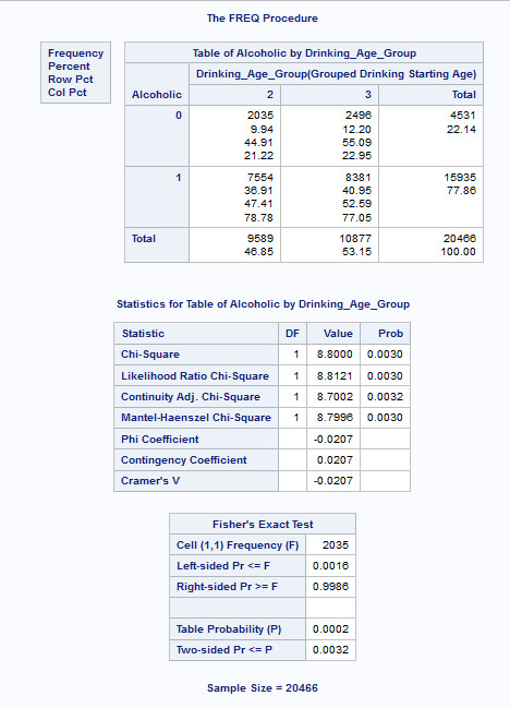
When examining the association between alcoholism (categorical response variable) and the grouped drinking starting age (categorical explanatory variable), a chi-square test of independence revealed that those who started drinking young (drinking age group 1) are less likely alcoholics (44.95%) compared to 78.78% for drinking age group 2 and 77.05% for drinking age group 3.

At a p-value<0.0001 the null hypothesis that there is no association between the two variables is rejected and the alternative hypothesis accepted.

As there are 3 categories for the explanatory variable pairwise comparisons were conducted to protect against Type 1 error. With the three comparisons conducted, the Bonferroni-adjusted p-value is reduced to (0.05/3=0.017).

The three pairwise comparisons all revealed a p-value smaller than 0.017 (<0.0001 for categories 1 and 2, <0.0001 for categories 1 and 3, and 0.003 for categories 2 and 3),  which indicates that all three groups are different from each other.

[jane-doe-coursera-blog]

2. Week 1 Assignment

I am investigating whether there is a connection between the family history of alcoholism and the level of alcohol that an individual consumes. I am thus running an Analysis of Variance (ANOVA). The null hypothesis is thus that there is no connection between the family history and the number of months during which an individual drank in the past 12 months, whereas the alternative hypothesis is that there is a relationship between the two variables.

I ran an ANOVA procedure on the two variables „family_history“ which is a categorical variable that takes on the values of yes and no and S2AQ8A, which is the number of months in which an individual drank alcohol in the past 12 months and thus ranges from 0 to 12. We can see that the mean number of months that individuals without a family history of alcoholism drink is 6.02 and the mean for those with alcohol-dependent family members is 5.93 with a standard deviation of 2.7 for both respectively. The p-value is 0.0216, which suggests rejecting the null hypothesis and accepting the alternative hypothesis to conclude that there is a significant association between family history and drinking habits. We can conclude that individuals with a family history of alcoholism drink on fewer occasions than those without a family history.

I further ran a second ANOVA procedure with a categorical explanatory variable (the age group when an individual first started drinking) that has more than two categories. The results are found below. We can reject the null hypothesis that all means are equal.

To determine which means are not equal a Duncan’s Multiple Range Test was run. The results are below. We can see that for all three age groups the bars are not overlapping. This shows that all means are significantly different from the other two, respectfully. We can hence conclude that each age group reported significantly different drinking frequencies. Those who started drinking below the age of 18 drank the least in the past twelve months, those who started after they turned 21 drank the most.

The code that contains the ANOVA models can be found below.

[jane-doe-coursera-blog]

A sample of 36,309 noninsitutionalized individuals that are representative for the United States civilian population of 18 years and older was questioned about alcohol and drug disorders, related risk factors, and associated physical as well as mental disabilities.

They were for example asked if they are a current drinker, an ex-drinker or a lifetime abstainer as well as how often they drank alcohol in the past twelve months. I chose a subset of the data by limiting my sample to those who consider themselves a current or ex-drinker and have drunk alcohol in the past 12 months. As there are no individuals who stopped drinking in the past twelve months, there are only 26741 current drinkers in the subset.

For data management purposes, I further created a secondary variable called “AGE_DIFF_DRINKING”. It measures the difference between the age when the individual started drinking once a week and the age he or she started drinking at all. I hope it will give me an indication of how fast a person progresses towards alcoholism. I also created the variable “Number_Alcoholic_Family_Membs”, which takes on values between 0 and 6 depending on how many close family members (parents and grandparents) were alcoholics and the variable “Family_History”, which simply indicates whether there is an alcoholic family member.

I include univariate graphs for the three variables. You can see that about 65% reported no alcoholic family member and that 35% reported an alcoholic family member. If we take the individual answers and exclude everyone who answered unknown to any of the family member we can count the number of alcoholic family members. Roughly, 21% reported one alcoholic family member and 9969 individuals were excluded due to missing values. The graph is unimodal with a mode at 0 and a spread of 6. It is thus right-skewed.

The years between the time an individual started to drink and the time when they started to drink once a week are presented in the second bar chart. You can see that the mode is 0 and that it is also right-skewed with a spread of 73.

When we graph these two variables together, we need a bivariate bar chart as none of the variables are continuous. The result is as expected: The more alcohol-dependent family members an individual has, the less time passes between their first drink and the time when they start drinking once a week. For those without alcoholic family members the mean is 4.2 years, for those with 6 alcohol-dependent family members, the mean is 1.3 years. The trend is not perfect, but very clear.

[jane-doe-coursera-blog]

A sample of 36,309 noninsitutionalized individuals that are representative for the United States civilian population of 18 years and older was questioned about alcohol and drug disorders, related risk factors, and associated physical as well as mental disabilities.

They were for example asked if they are a current drinker, an ex-drinker or a lifetime abstainer as well as how often they drank alcohol in the past twelve months. I chose a subset of the data by limiting my sample to those who consider themselves a current or ex-drinker and have drunk alcohol in the past 12 months. As there are no individuals who stopped drinking in the past twelve months, there are only 26741 current drinkers in the subset.

For data management purposes, I set aside missing data. There was the option to answer “Unknown” in a number of questions, coded in as either 99 in the case of numerical answers, such as “How often do you drink?” or as 9 in the case of questions such as “Was your father an alcoholic”. As theses answers do not represent a legitimate category, they were coded as missing values. I have included the results for the question “How often did you drink in public during the past 12 months. It becomes obvious that instead of an answer choice 99, 142 values are now missing.

It did not make sense for me to code in valid data as there were no legitimate skips because I had already excluded non-drinkers previously in the research question.

I further created a secondary variable called “AGE_DIFF_DRINKING”. It measures the difference between the age when the individual started drinking once a week and the age he or she started drinking at all. I hope it will give me an indication of how fast a person progresses towards alcoholism. It becomes clear that most individuals started drinking once a week the same year they started drinking [39.6%] and that there are 10605 missing values for those who did not report one or both of the starting ages. (I had to split the output for this one for better readability.)

Lastly, I grouped two age variables into categories: the age when started drinking and the age when started drinking once a week. I display the frequency tables for the first. Group 1 includes those who started drinking before the age of 18 (i.e. before they are of legal age); Group 2 includes those who started drinking between the ages of 18 and 20 (i.e. before they are of legal drinking age in the U.S.) and Group 3 includes those who started drinking after turning 21. Roughly one third can be found in each group and there are 2029 missing observations (including those who answered unknown).

[jane-doe-coursera-blog]

A sample of 36,309 noninsitutionalized individuals that are representative for th United States civilian population of 18 years and older was questioned about alcohol and drug disorders, related risk factors, and associated pyhsical as well as mental disabilities.

They were for example asked if they are a current drinker, an ex-drinker or a lifetime abstainer as well as how often they drank alcohol in the past twelve months. I chose a subset of the data by limiting my sample to those who consider themselves a current or ex-drinker and have drunk alcohol in the past 12 months. As there are no individuals who stopped drinking in the past twelve months, there are only 26741 current drinkers in the subset.

It was further asked how of ten they drank alcohol in the past year. Of those that answered the question, most (13.6%) fell into category 10 [1 or 2 times in the last year]. The second most frequent category was chosen by 13.3% [2 to 3 times a month].

Because I am interested in investigating whether the family history affects the drinking pattern I included variables on alcohol-dependent family members. 20.65% of the subset reported that their father was alcoholic [category 1], while only 6.11% reported an alcohol-dependent mother [category 1]. 5.08% and 2.16% reported that they did not know the answer [category 9].

[jane-doe-coursera-blog]

Literature Review: Family History and Alcoholism

After reviewing the NESARC code book, I found myself interested in the alcohol drinking pattern. Thus, I have saved the variables of Section 2A to my personal codebook.

As I have relatives who struggle with alcohol dependence, I care most about the association between the history of the family with alcoholism and alcohol consumption of an individual and aim at answering the research question whether the alcohol consumption of an individual is associated with the individual’s family history of alcohol dependence. Hence, I added the variables of Section 2D to my code book.

There have been extensive studies on the association between family history and alcohol abuse. To perform a review on the literature, search terms included “family history”, “family predisposition” and “genetics” in combination with “alcohol dependence”, “alcoholism” and “alcohol consumption”. In the simplest way, subjects can be designated as family history negative (FH-) if they report no history of alcoholism in their family. This can be narrowly defined at parent-level or wider including grand-parents, aunts and uncles and so forth. On the contrary, if the subject reports alcohol abuse within the defined family range, he or she would be classified as family history positive (FH+).

There are different research angles to capture this association. One strand looks at the genetics of alcohol dependence. In a study of 8,296 relatives of alcoholic probands and 1,654 controls, Nurnberger et al. (2004) found that the risk of the relatives is increased approximately two-fold for FH+ individuals. Factors that were thought to possibly further influence the effects of a family history of alcoholism are gender and degree of kinship. In this context, Kaij and Dock (1975) previously found that the gender of the alcoholic does not play a role in determining the risk of dependence in relatives. This was further reinforced in the findings of a study by Cloninger, Bohman and Sigvardsson in 1981. The degree of kinship, however, was found to impact the risk of alcohol dependence. Dawson, Harford, and Grant (1992) found that risk increase by 45% for second or third degree relatives, by 86% for first degree relatives and by 167% for first and second or third degree relatives.

Another research strand explores environmental factors related to family history of alcoholism, such as the amount of drinking in the environment and nurturance in the social support system that can be thought of as indirectly, but not directly associated with the family’s history of alcohol abuse. Schuckit and Smith (2000) found that for their sample of 315 sons of alcoholics, the former variables added significantly to the explanatory power of their model. Similarly, Grant (1998) explored not only family dependence, but also age at first alcohol use and found the latter to increase the risk of becoming alcohol dependent.

Further, family history seems to have an effect on the individual’s readiness to admit to alcohol problems. Lewis and Nixon (2013) found that women in treatment were more likely to be FH+ than men, indicating that possibly women are more likely to seek treatment for alcohol abuse based on experiences within their family. The same was true for spousal alcohol abuse. However, their sample consisted of 531 patients in treatment and thus does not account for non-treatment-seeking subjects.

Concluding, it can be stated that family history of alcohol abuse as well as environmental factors indirectly related to that history, seem to greatly increase a person’s risk of alcohol dependence. Across studies, however, the common theme is that, FH+ individuals have by far a greater risk of alcohol dependence than FH- individuals even after controlling for environmental factors. I hence want to focus on the family history and its impact on not only the risk of alcoholism in individuals, but also on how that history impacts drinking patterns, such as how often a person drinks, where a person usually drinks and how much a person usually drinks. Concerning family history, I intend to distinguish degrees of kinship and natural vs. adoptive or marital relationships. The hypothesis is that the more family members are alcohol-dependent, the more probable it is that the individual exhibits drinking patterns related to alcoholism (more drinks, drinking at home alone, frequent drinking, etc.).

Sources used:

Cloninger, C., Bohman, M. and Sigvardsson, S. (1981). Inheritance of Alcohol Abuse. Archives of General Psychiatry, 38(8), pp.861-868.

Dawson, D., Harford, T. and Grant, B. (1992). Family History as a Predictor of Alcohol Dependence. Alcoholism: Clinical and Experimental Research, 16(3), pp.572-575.

Grant, B. (1998). The Impact of a Family History of Alcoholism on the Relationship Between Age at Onset of Alcohol Use and DSM - IV Alcohol Dependence: Results From the National Longitudinal Alcohol Epidemiologic Survey. Alcohol Health and Research World, 22(2), p.144.

Kaij, L. and Dock, J. (1975). Grandsons of Alcoholics. Archives of General Psychiatry, 32(11), pp.1379-1381.

Lewis, B. and Nixon, S. (2013). Characterizing Gender Differences in Treatment Seekers. Alcoholism: Clinical and Experimental Research, 38(1), pp.275-284.

Nurnberger, J., Wiegand, R., Bucholz, K., O’Connor, S., Meyer, E., Reich, T., Rice, J., Schuckit, M., King, L., Petti, T., Bierut, L., Hinrichs, A., Kuperman, S., Hesselbrock, V. and Porjesz, B. (2004). A Family Study of Alcohol Dependence. Archives of General Psychiatry, 61(12), pp.1246-1256.

Schuckit, M. and Smith, T. (2000). The relationships of a family history of alcohol dependence, a low level of response to alcohol and six domains of life functioning to the development of alcohol use disorders. Journal of Studies on Alcohol, 61(6), pp.827-835.