jparkau

[jparkau]

K-means Cluster Analysis

In order to create groups of similar bottles of wine, we conducted a k-means cluster analysis and found subgroups of wines based on the similarity of responses on 11 variables. Clustering variables included quantitative variables (which work best on k means analysis): fixed acidity, volatile acidity, citric acid, residual sugar, chlorides, free sulfur dioxide, total sulfur dioxide, density, pH, sulphates, and alcohol level.

CODE:

Call in the libraries.

from pandas import Series, DataFrame import pandas as pd import numpy as np import matplotlib.pylab as plt from sklearn.model_selection import train_test_split from sklearn import preprocessing from sklearn.cluster import KMeans

Call in the data (I used kaggle.com to retrieve the data) data = pd.read_csv("redwinequality.csv")

Make all Dataframe columns uppercase data.columns = map(str.upper, data.columns)

Clean the dataset and delete all of the data with missing information

data_clean = data.dropna()

Assign the following clustering variables cluster=data_clean[['FIXED','VOLATILE','CITRIC','RESSUGAR','CHLORIDES','FSDIO', 'TSDIO','DENSITY','PH','SULPHATES','ALCOHOL']] cluster.describe()

Standardize clustering variables to have mean=0 and sd=1, because the variables should have the same scale to be fair. Astype float 64 ensures numeric format. clustervar=cluster.copy() for col in ['FIXED','VOLATILE','CITRIC','RESSUGAR','CHLORIDES','FSDIO', 'TSDIO','DENSITY','PH','SULPHATES','ALCOHOL']:    clustervar[col] = preprocessing.scale(clustervar[col].astype('float64'))

Split data into train and test sets. We set 30% of the data set into the testing set and 70% into training. clus_train, clus_test = train_test_split(clustervar, test_size=.3, random_state=123)

Perform K-means cluster analysis for 1-9 clusters. We use Euclidean distance to measure similarity.                                             from scipy.spatial.distance import cdist clusters=range(1,10) meandist=[]

for k in clusters:    model=KMeans(n_clusters=k)    model.fit(clus_train)    clusassign=model.predict(clus_train)    meandist.append(sum(np.min(cdist(clus_train, model.cluster_centers_, 'euclidean'), axis=1))    / clus_train.shape[0])

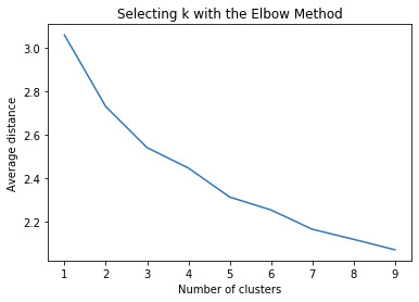
In order to see how many clusters we should choose from, we plot average distance from observations from the cluster centroid and use the Elbow Method.

plt.plot(clusters, meandist) plt.xlabel('Number of clusters') plt.ylabel('Average distance') plt.title('Selecting k with the Elbow Method')

We assume that we choose 3 clusters. Because this is a subjective conclusion, let us interpret the k=3 clustering. model3=KMeans(n_clusters=3) model3.fit(clus_train) clusassign=model3.predict(clus_train)

Use canonical discriminant analysis, which will reduce the number of clustering variables. Plot the first two most influential canonical variables to see the discriminant plot and see cluster within variance as well as overlapping points.

from sklearn.decomposition import PCA pca_2 = PCA(2) plot_columns = pca_2.fit_transform(clus_train) plt.scatter(x=plot_columns[:,0], y=plot_columns[:,1], c=model3.labels_,) plt.xlabel('Canonical variable 1') plt.ylabel('Canonical variable 2') plt.title('Scatterplot of Canonical Variables for 3 Clusters') plt.show()

We can now merge cluster assignment with clustering variables to examine the cluster variable means by cluster clus_train.reset_index(level=0, inplace=True) cluslist=list(clus_train['index']) labels=list(model3.labels_) newlist=dict(zip(cluslist, labels)) newlist newclus=DataFrame.from_dict(newlist, orient='index') newclus newclus.columns = ['cluster']

newclus.reset_index(level=0, inplace=True) # merge the cluster assignment dataframe with the cluster training variable dataframe # by the index variable merged_train=pd.merge(clus_train, newclus, on='index') merged_train.head(n=100) # cluster frequencies merged_train.cluster.value_counts()

We can now calculate clustering variable means by cluster clustergrp = merged_train.groupby('cluster').mean() print ("Clustering variable means by cluster") print(clustergrp)

To validate clusters in training data, we can examine the cluster differences in QUALITY using ANOVA quality_train, quality_test = train_test_split(quality_data, test_size=.3, random_state=123) quality_train1=pd.DataFrame(quality_train) quality_train1.reset_index(level=0, inplace=True) merged_train_all=pd.merge(quality_train1, merged_train, on='index') sub1 = merged_train_all[['QUALITY','cluster']].dropna()

import statsmodels.formula.api as smf import statsmodels.stats.multicomp as multi

qualitymod = smf.ols(formula='QUALITY ~ C(cluster)', data=sub1).fit() print (qualitymod.summary())

print ('means for QUALITY by cluster') m1= sub1.groupby('cluster').mean() print (m1)

print ('standard deviations for QUALITY by cluster') m2= sub1.groupby('cluster').std() print (m2)

mc1 = multi.MultiComparison(sub1['QUALITY'], sub1['cluster']) res1 = mc1.tukeyhsd() print(res1.summary())

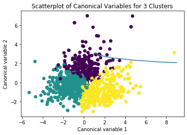
By visualizing the elbow method, we can see that k=2 or k=3 will be an appropriate number of clusters. To further analyze this, let us use the canonical discriminant analyses to interpret the k=3 cluster solution. The canonical discriminant analyses reduced the 11 clustering variables down to 5 that affected most of the variance in clustering variables. We then plot the 2 most influential canonical variables on a scatterplot and see the density or overlap between the points.

We can see from the scatterplot that clusters 1 and 2 are all densely packed with relatively low within cluster variance. Cluster 3 was generally distinct, but the observations had greater spread than cluster 1 and 2 which suggests that it has a higher within cluster variance. Clusters 1, 2, and 3 do not overlap with one another very much. The plot does suggest that a 2 cluster solution is also feasible.

The means on the clustering variables show that compared to the other clusters, types of wine in cluster 1 are low in fixed and volatile acidity, while cluster 2 are low in fixed but relatively higher in volatile acidity. Wine types in cluster 3 are high in fixed acidity and lower in volatile acidity. This indicates that wines in cluster 1 are not acidic, while cluster 2 wine types are not acidic but tend to vary as time continues, and cluster 3 wine types are acidic but tend to vary with time. Both cluster 1 and 3 are low in pH (with cluster 3 being more), while cluster 2 is higher in pH. Wines low in sulphates include cluster 1 and 2, while cluster 1 has a lower alcohol level than others.

In order to externally validate the clusters, we conducted an Analysis of Variance to test for significant differences between the clusters on Quality. We used the turkey test for post hoc comparisons between the clusters, and the results showed us moderate differences between the clusters on Quality (although not significant). On a scale of 10, cluster 2 had similar quality means compared to cluster 1 and 3, with cluster 2 quality mean being 5.56 and cluster 1 and 3’s quality means being 5.375 and 5.972 respectively. When comparing cluster 1 and 3 there is a more noticeable difference in quality mean. Wine in cluster 1 is the lowest in quality, while wine in cluster 3 is the highest in wine quality.

[jparkau]

Lasso Regression Analysis

In order to answer the question: which factors of the coffee beans will affect the quality? I used the data given by Coffee Quality Institute (taken from kaggle.com). In this example, we conducted the lasso regression analysis to see which of the 21 categorical and quantitative predictor variables would best predict the quantitative response variable measuring the quality of coffee bean. I included the following categorical predictors: Species (binary categorical: Arabica / Robusta), variety (Caturra, Bourbon, Other), processing method (Natural / Dry, Washed / Wet, Other). Quantitative predictor variables include the aroma, flavor, aftertaste, acidity, body, balance, uniformity, cup cleanliness, sweetness, moisture, quakers, category 1 defects, and category 2 defects.

CODE:

First we import the libraries.

import pandas as pd import numpy as np import matplotlib.pylab as plt from sklearn.model_selection import train_test_split from sklearn.linear_model import LassoLarsCV

Then we load the dataset. I took mine from the Coffee Quality Institute. data = pd.read_csv("coffee2.csv")

Make all datafram columns uppercase. data.columns = map(str.upper, data.columns)

Clean the data and make sure that any missing information is dropped from our analyses. data_clean = data.dropna()

Select the predictor variables. predvar= data_clean[['ARABICA','ROBUSTA','CATURRA','BOURBON','OTHVAR','WW', 'ND','OTHPRO','AROMA','FLAVOR', 'AFTERTASTE','ACIDITY','BODY','BALANCE','UNIFORMITY','CLEANCUP','SWEET', 'MOIST','QUAKERS','CATONEDEF','CATTWODEF']]

Select the target variables

target = data_clean.CUPPERPOINT

Standardize the predictors to have mean=0 and sd=1 (because the penalty term is not fair if the predictors are not on the same scale). float 64 code ensures that the predictors will have a numeric format.

predictors=predvar.copy() from sklearn import preprocessing for col in ['ARABICA','ROBUSTA','CATURRA','BOURBON','OTHVAR','WW', 'ND','OTHPRO','AROMA','FLAVOR', 'AFTERTASTE','ACIDITY','BODY','BALANCE','UNIFORMITY','CLEANCUP','SWEET', 'MOIST','QUAKERS','CATONEDEF','CATTWODEF']:    predictors[col] = preprocessing.scale(predictors[col].astype('float64'))

Split the data into training and testing sets (I put 30 percent into the test set and 70 to training set). pred_train, pred_test, tar_train, tar_test = train_test_split(predictors, target,                                                              test_size=.3, random_state=123)

Use the Lasso Regression Model and let cv=10. This means we perform a k-fold cross validation with 10 random folds from the training data set to choose the final statistical model. model=LassoLarsCV(cv=10, precompute=False).fit(pred_train,tar_train)

Print variable names and regression coefficients print(dict(zip(predictors.columns, model.coef_)))

Plot coefficient progression m_log_alphas = -np.log10(model.alphas_) ax = plt.gca() plt.plot(m_log_alphas, model.coef_path_.T) plt.axvline(-np.log10(model.alpha_), linestyle='--', color='k',            label='alpha CV') plt.ylabel('Regression Coefficients') plt.xlabel('-log(alpha)') plt.title('Regression Coefficients Progression for Lasso Paths')

Plot mean square error for each fold m_log_alphascv = -np.log10(model.cv_alphas_) plt.figure() plt.plot(m_log_alphascv, model.mse_path_, ':') plt.plot(m_log_alphascv, model.mse_path_.mean(axis=-1), 'k',         label='Average across the folds', linewidth=2) plt.axvline(-np.log10(model.alpha_), linestyle='--', color='k',            label='alpha CV') plt.legend() plt.xlabel('-log(alpha)') plt.ylabel('Mean squared error') plt.title('Mean squared error on each fold')

Show the MSE from training and test data from sklearn.metrics import mean_squared_error train_error = mean_squared_error(tar_train, model.predict(pred_train)) test_error = mean_squared_error(tar_test, model.predict(pred_test)) print ('training data MSE') print(train_error) print ('test data MSE') print(test_error)

Show R-square from training and test data rsquared_train=model.score(pred_train,tar_train) rsquared_test=model.score(pred_test,tar_test) print ('training data R-square') print(rsquared_train) print ('test data R-square') print(rsquared_test)

OUTPUT:

{'ARABICA': 0.0, 'ROBUSTA': 0.0, 'CATURRA': 0.014651466879184293, 'BOURBON': 0.0, 'OTHVAR': 0.0, 'WW': 0.0, 'ND': 0.02404759141496131, 'OTHPRO': 0.0, 'AROMA': 0.03668228465812958, 'FLAVOR': 0.1057058683637391, 'AFTERTASTE': 0.10615286256402166, 'ACIDITY': 0.023956287190667554, 'BODY': 0.027815903709025872, 'BALANCE': 0.04938996327406754, 'UNIFORMITY': 0.0, 'CLEANCUP': 0.006628593931969668, 'SWEET': 0.0, 'MOIST': -0.00990557690970148, 'QUAKERS': 0.0, 'CATONEDEF': 0.0, 'CATTWODEF': 0.0} training data MSE 0.04823858697500274 test data MSE 0.0483824754084936 training data R-square 0.6901460832830091 test data R-square 0.6722367888954521

INTERPRETATION:

Of the 21 predictor variables, 10 were retained in the selected model. We can see from the output, that the quality of coffee beans is most strongly associated with the flavor and aftertaste, followed by the balance and aroma. All of the chosen predictors were positively associated with coffee bean quality except for the moisture (which had a coefficient of around -0.0099). Other predictors associated with greater quality of coffee bean included Caturra variety coffee beans, natural / dry processing methods, acidity, body, and cup cleanliness. The coefficient of the rest of the variables became zero in the shrinking process.

By looking at the mean squared error of the training nd testing data, we can see that the testing data has a slightly higher mean squared error, but overall the two values are close to each other. The R-square of the data indicates that the selected model can explain 69% and 67% variance of the training and testing data.

[jparkau]

Random Forest Analysis

To figure out the most important variable that affects whether or not a client will default on their loan, we performed the random forest analysis and evaluated the importance of each explanatory variable in predicting the binary, categorical response variable. I included the following explanatory variables as candidates: amount of the loan requested (LOAN), amount due on existing mortgage (MORTDUE), value of current property (VALUE), reason for debt (DebtCon or HomeImp), Job (6 categories: professional executive, manager , office, salesperson, works by themselves, and other miscellaneous jobs) years at present job (YOJ), number of major derogatory reports (DEROG), number of delinquent credit lines (DELINQ), age of oldest trade line in months (CLAGE), number of recent credit lines (NINQ), number of total credit lines (CLNO), debt-to-income ratio (DEBTINC).

Code:

First, import the libraries.

from pandas import Series, DataFrame import pandas as pd import numpy as np import os import matplotlib.pylab as plt from sklearn.model_selection import train_test_split from sklearn.tree import DecisionTreeClassifier from sklearn.metrics import classification_report import sklearn.metrics # Feature Importance from sklearn import datasets from sklearn.ensemble import ExtraTreesClassifier

Next, we can load the dataset. I chose the dataset from kaggle.com (https://www.kaggle.com/ajay1735/hmeq-data)

AH_data = pd.read_csv("default.csv")

Clean the data by leaving out the omitted information.

data_clean = AH_data.dropna()

data_clean.dtypes data_clean.describe()

Then, we can now assign the target and explanatory variables. Assign the predictors or explanatory variables.

predictors = data_clean[['LOAN','MORTDUE','VALUE','HomeImp','DebtCon','ProfExe','Mgr','Office','Sales', 'Self','Other','YOJ','DEROG','DELINQ','CLAGE','NINQ','CLNO','DEBTINC']]

Set the target to be the column indicating defaults.

targets = data_clean.BAD

Split and shape the dataset into training and testing set. I assigned 40 percent of the data set to testing and 60% to training.

pred_train, pred_test, tar_train, tar_test  = train_test_split(predictors, targets, test_size=.4)

pred_train.shape pred_test.shape tar_train.shape tar_test.shape

We can first import the Random Forest model from sklearn.

from sklearn.ensemble import RandomForestClassifier

Then we can set the number of trees to 25 and fit the data sets.

classifier=RandomForestClassifier(n_estimators=25) classifier=classifier.fit(pred_train,tar_train)

Next we can predict the test set.

predictions=classifier.predict(pred_test)

We can see the confusion matrix and accuracy score of the random forest.

sklearn.metrics.confusion_matrix(tar_test,predictions) sklearn.metrics.accuracy_score(tar_test, predictions) my_conf_matrix = sklearn.metrics.confusion_matrix(tar_test, predictions)

Remember to print out the confusion matrix and accuracy score to see the results when you run the model.

print('confusion matrix')

print (my_conf_matrix)

my_accurate_score = sklearn.metrics.accuracy_score(tar_test, predictions)

print('Accuracy score')

print(my_accurate_score)

We can then fit an extra tree model to the data. model = ExtraTreesClassifier() model.fit(pred_train,tar_train)

Print out the relative importance of each variable or feature. print(model.feature_importances_)

In order to see whether or not we needed 25 trees to attain the level of accuracy, we can run a different number of trees and see the effect.

trees=range(25) accuracy=np.zeros(25)

for idx in range(len(trees)):   classifier=RandomForestClassifier(n_estimators=idx + 1)   classifier=classifier.fit(pred_train,tar_train)   predictions=classifier.predict(pred_test)   accuracy[idx]=sklearn.metrics.accuracy_score(tar_test, predictions)

plt.cla() plt.plot(trees, accuracy)

OUTCOME:

confusion matrix [[1222    0] [  75   49]] Accuracy score 0.9442793462109955 [0.08024514 0.07817877 0.08530594 0.01802502 0.01708088 0.01065729 0.01518857 0.01421459 0.01146578 0.01118814 0.01559736 0.06978823 0.06903367 0.0928835  0.09667542 0.06849764 0.08892933 0.15704473]

THOUGHTS:

DEBTINC or Debt-to-income ratio had the highest relative importance score of 0.15704473 out of all of the explanatory variables. The other variables were (in order of decreasing importance): age of oldest trade line in months, number of delinquent credit lines. The rest of the explanatory variables had a relative important score of less than 0.09. The confusion matrix tells us there are 0 cases of false positives and 75 cases of false negatives. The accuracy of the random forest was 94.43%, while a single tree would have given an accuracy of around 93% (given by the plot). The difference is quite small meaning that the growing of multiple trees adds little overall accuracy of the model, which could indicate that a single tree may be appropriate. (Although if I preferred a 2% more accurate model, I could simply use 5 trees, because according to the plot, the accuracy score seems to level off after 5 trees.) 

[jparkau]

Classification Tree Analysis

In this assignment, I used a decision tree to test the relationship between the explanatory variables and a binary, response variable. The research question I attempted to experiment with was: which client will default on their loans?

I used the following explanatory variables to contribute information to the classification evaluating whether or not a client of a bank will default on their loans: amount of the loan requested (LOAN), amount due on existing mortgage (MORTDUE), value of current property (VALUE), reason for debt (DebtCon or HomeImp), Job (6 categories: professional executive, manager , office, salesperson, works by themselves, and other miscellaneous jobs) years at present job (YOJ), number of major derogatory reports (DEROG), number of delinquent credit lines (DELINQ), age of oldest trade line in months (CLAGE), number of recent credit lines (NINQ), number of total credit lines (CLNO), debt-to-income ratio (DEBTINC).

Code:

First, import the libraries.

from pandas import Series, DataFrame

import pandas as pd

import numpy as np

import os

import matplotlib.pylab as plt

from sklearn.model_selection import train_test_split

from sklearn.tree import DecisionTreeClassifier

from sklearn.metrics import classification_report

import sklearn.metrics

Next, we can load the dataset. I chose the dataset from kaggle.com (https://www.kaggle.com/ajay1735/hmeq-data)

#Load the dataset

AH_data = pd.read_csv("default.csv")

Clean the data by leaving out the omitted information.

data_clean = AH_data.dropna()

data_clean.dtypes

data_clean.describe()

Then, we can now assign the target and explanatory variables. Assign the predictors or explanatory variables.

predictors = data_clean[['LOAN','MORTDUE','VALUE','HomeImp','DebtCon','ProfExe','Mgr','Office','Sales', 'Self','Other','YOJ','DEROG','DELINQ','CLAGE','NINQ','CLNO','DEBTINC']]

Set the target to be the column indicating defaults.

targets = data_clean.BAD

Split the dataset into training and testing set. I assigned 40 percent of the data set to testing and 60% to training.

pred_train, pred_test, tar_train, tar_test  =   train_test_split(predictors, targets, test_size=.4)

pred_train.shape

pred_test.shape

tar_train.shape

tar_test.shape

At last, we can build the decision tree model (with max depth 3) on the training set and try out the prediction on the testing set.

classifier=DecisionTreeClassifier(max_depth = 3)

classifier=classifier.fit(pred_train,tar_train)

predictions=classifier.predict(pred_test)

Now create the confusion matrix using the code below.

sklearn.metrics.confusion_matrix(tar_test,predictions)

sklearn.metrics.accuracy_score(tar_test, predictions)

We can display the decision tree by using the code below.

from sklearn import tree

#from StringIO import StringIO

from io import StringIO

#from StringIO import StringIO

from IPython.display import Image

out = StringIO()

tree.export_graphviz(classifier, out_file=out, feature_names=predictors.columns, filled=True, rounded=True, special_characters=True)

import pydotplus

print(out.getvalue())

graph=pydotplus.graph_from_dot_data(out.getvalue())

Img=(Image(graph.create_png()))

display(Img)

graph.write_png("loandefault.png")

To view the confusion matrix, we can print it out.

my_conf_matrix = sklearn.metrics.confusion_matrix(tar_test, predictions)

print('confusion matrix')

print (my_conf_matrix)

We can also see the accuracy score using the code below.

my_accurate_score = sklearn.metrics.accuracy_score(tar_test, predictions)

print('Accuracy score')

print(my_accurate_score)

The first variable to split the sample into two subgroups was the debt to income ratio. Clients with a debt to income ratio less than or equal to 43.705 were more likely to default on their loans compared to clients who have a debt to income ratio higher than 43.705.

Out of the clients with a debt to income ratio less than or equal to 43.705, clients who have a number of delinquent credit lines less than or equal to 4.5 are more likely to default on their loans. The last subdivision is made with the variable LOAN, or the amount of loan borrowed from the bank. Clients who have requested a loan more than 4050 are more likely to default on their loans than those who have requested less. The final sample value = [1809, 124].

What does this all mean?

Findings: Under the assumption of 3 maximum nodes, we can note that the decision tree indicates that clients who have a debt to income ratio of less than or equal to 43.705, a number of delinquent credit lines less than or equal to 4.5, and who have requested a loan for more than 4050 are likely to default on their loans. The most important variables for classifying clients on their default loans are 1) Debt to Income Ratio, 2) number of delinquent credit lines, 3) amount of loans.

Confusion Matrix

[[1228   14]

[  78   26]]

Accuracy score

0.9316493313521546

The confusion matrix indicates that there are 14 cases of false positives and 78 cases of false negatives. The accuracy score is around 93% which is incredibly high (we perhaps need a bigger dataset).

Additional opinion: In my opinion, the data set might be too small to work with. I say this because the accuracy of the decision tree is incredibly high in terms of both bias and variance. However, when we look at the second subdivision, we can see that clients with a number of delinquent credit lines HIGHER than 4.5 are actually less likely to default on their loans. In reality, aren’t clients more prone to default on their loans if their credit lines are already labeled as delinquent? Perhaps this is a psychological issue, where people are more willing to learn from their previous mistakes. But in my opinion, seeing as the number of delinquent credit lines is actually used as a risk factor in many banks, we need a larger dataset to verify the second subdivision.