laketofountain

[laketofountain]

Binary - more than 1′s and 0′s - Logistic Regression Testing

In the final exercise for regression modeling we will look at regression testing for categorical variables - Logistic regression. We will use the data provided in the 2012 Outlook on Life Survey, carried out by the University of California, Irvine. Our focus area will be ‘ Feeling’ (OPTPES) - do you feel Optimistic or Pessimistic? This is a binary variable and will be used as our response variable. We will examine this using the explanatory variable  GENDER. Our hypothesis will ask the question - is Feeling related to Gender? We will also add political leaning to the regression test to determine if it is a confounding variable.

Results summary

The first regression test demonstrated that there was statistically no impact on feeling driven by gender - while the p value was < 0,0001 the Odds Ratio was 0.5 which would suggest that Optimism and Pessimism are driven by factors other than Gender. The second test added Political Leaning to the test. The odds ratio was even lower which suggested that it also had little to do with Feeling and was not a confounding variable.

Data Management

Activities were carried out to remove values not being tested and to re-code our binary variables assigning the values 1 and 0. 

The Leaning variable was a 7 value categorical variable which was collapsed into a Binary variable. Values 1-3 were assigned to Liberal (0) and values 5-7 were assigned to Conservative (1).

Regression Modeling

Our first model tests the association between Feeling and Gender. The p values are significant in that they are both less than 0.0001 however the 95% confidence intervals are both < 1 which shows that  Gender does not have a significant impact on feeling. The code to generate and model output follows .

Code:

Output:

The second model adds the explanatory variable Leaning - (Liberal or Conservative) to see if that has an impact on the hypothesis.  The p values again are significant in that they are both less than 0.0001 however the 95% confidence intervals are all still < 1 which shows that  the explanatory variable (Gender) will likely not impact the response variable (Feeling) when Leaning is accounted for. Feeling is not a confounding variable. The code to generate and model output follows .

Code:

Output:

[laketofountain]

Under the Influence

Testing a Multiple Regression Model

For this exercise I am using the Gapminder data set - based on a collection of Global health indicators gathered from multiple countries since 2005 by the Gapminder non profit organization based in Norway. For this exercise I am trying to establish if there is a relationship between Alcohol Consumption (explanatory variable - alcconsumption) and Life Expectancy (response variable - lifeexpectancy). I will then examine the relationship and see if Income Per Person (incomeperperson) is an confounding variable. 

First of all I centered my quantitative variables by subtracting the mean from each.

The linear scatter plot shown would appear to demonstrate  a relationship between Life Expectancy and Alcohol Consumption with a marked decrease as consumption units passes 15. To support this I ran a linear regression test to establish whether or not there is a relationship between the Response Variable - Life Expectancy and the explanatory variable Alcohol Consumption. You can see from the results below that the p value is < 0.05 and the parameter estimate (Beta coefficient) value is positive suggesting that Alcohol consumption does indeed have an impact on Life Expectancy. 

Next I added the Income Per Person variable and ran a multiple regression model  to see if it is possible that this is a confounding variable - i.e. is Life Expectancy driven by Income and not impacted by Alcohol consumption? The results show a positive parameter estimate (Beta Coefficient) value and a p value <0.05 for both variables which suggest that they both have an impact on Life Expectancy however Income Per Person is not a confounding variable.

The Q-Plot and Standardized Residual Plots for the variables follow

The Q plot shows that our values do not quite follow a linear plot - they vary slightly across the distribution. This suggests that there could be explanatory variables that have a more direct impact on the response variable - Life Expectancy.

The standardized residual plot shows that fewer than 95% of the residuals fall no more than 2 standard deviations from the mean, In this case we see more than 5% of the residuals outside that tolerance meaning that there are outliers present that may be impacting the results. This would also suggest a poor model fit so we may be missing an important explanatory variable.

The Leverage /  Influence Plot

Our Influence plot reinforces the outliers that we see in our standardized residual plot. We have multiple residuals that have high leverage on the model suggesting better choice of variables would help prove our hypothesis. In this case our hypothesis that Alcohol Consumption and Life Expectancy are related is not supported by income level.

[laketofountain]

Linear Regression Model Testing

In exercise two of the ‘Regression Modeling in Practice’  module I will be testing for a relationship between the Average Monthly Income (Response Variable) of a respondent and whether or not they have Optimistic or Pessimistic outlook (Explanatory Variable) based on the data provided in the 2012 Outlook on Life survey, carried out by the University of California, Irvine. 

The Optimistic / Pessimistic variable OPTPES is a re-coded version of the variable W2_QE1 - which describes whether or not the respondent is Optimistic (1) or Pessimistic (2). The re-code sets the value for pessimistic to 0 to support the linear regression model. this variable is categorical so we will not be centering against the mean in this exercise.

First of all I verified the sample size for respondents (total 1110).

Then we re-code the variable as follows to realign pessimism with the value 0.

Once completed I verified that the re-code was successful

generating the output:

Once the OPTPES variable had been managed monthly income is addressed. 

The re-code creates AVMONTHLYINC - 19 average monthly income amounts (not all shown in the cut and paste above) based on the income bands in the survey. To determine the amount the lower and upper annual band were added together and divided by 2. This was then divided by 12 to get the monthly equivalent.

Once the two variables were managed a regression model was run with OPTPES as the Explanatory Variable and AVMONTHLYINC as the Response Variable.

This produces the Linear Regression Model below

It can be seen from the results that we can accept the null hypothesis that there is little or no relationship between our feeling variable OPTPES and Average Monthly Income AVMONTHLYINC - with a Beta of 1.335 and p = 0.248 we are outside the p = 0.05 tolerance that would enable us to reject the null hypothesis. The bi-variate bar graph shown demonstrates this as well - there is little difference between the average income and feeling variables across the survey.

A very happy new year to whoever is lucky enough to review this blog!

A complete listing of the program follows 

# -*- coding: utf-8 -*- """ Spyder Editor

This is a temporary script file. """ import pandas import numpy import seaborn import matplotlib.pyplot as plt import matplotlib.patches as mpatches import statsmodels.formula.api as smf import statsmodels.stats.multicomp as multi import statsmodels.api

data = pandas.read_csv('ool_pds.csv', low_memory=False)

#Set PANDAS to show all columns in DataFrame pandas.set_option('display.max_columns', None) #Set PANDAS to show all rows in DataFrame pandas.set_option('display.max_rows', None)

# bug fix for display formats to avoid run time errors pandas.set_option('display.float_format', lambda x:'%f'%x)

#convert fields of interest to numberic type #Can optimism and political affiliation be linked?

#ARE YOU OPTIMISTIC? data["W2_QE1"] = pandas.to_numeric((data["W2_QE1"]),errors='coerce') #PERSONAL BELIEF - CONSRVATIVE or LIBERAL data["W1_C2"] = pandas.to_numeric((data["W1_C2"]),errors='coerce') #HOUSE OWNERSHIP data["PPRENT"] = pandas.to_numeric((data["PPRENT"]),errors='coerce') #HOUSEHOLD INCOME data["PPINCIMP"] = pandas.to_numeric((data["PPINCIMP"]),errors='coerce') #lowercase data.columns = map(str.upper, data.columns)

#DATA MANAGEMENT

#Create data subset #Include only data for optimists and pessimists

#Make a copy for manipulation sub200 = data.copy()

#DATA MANAGEMENT FOR FEELING - OPTIMIST/PESSIMIST; #SUBSET 1: Remove data for those who are neither optimists nor pessimists (or non responses) - feeling data sub200=data[(data['W2_QE1']>=1) & (data['W2_QE1']<3)]

#Frequency Table for Feeling data print ('Frequency Table Check for feeling data prior to recode') print ('1.000000 - Optimistic 2.000000 - Pessimistic') print (" ")

chk1 = sub200['W2_QE1'].value_counts(sort=False, dropna=False) chk1 = chk1.sort_index(ascending=True) print (chk1)

#create feeling column with values 1 (Optimistic) or 0 (Pessimistic) for Explanitory Response Variable recode1 = {1:1, 2:0} sub200['OPTPES']= sub200['W2_QE1'].map(recode1)

# check recode for feeling print ('Frequency Table Check for Recode - 0 Pessimistic / 1 Optimistic') print (" ") chkrc1 = sub200['OPTPES'].value_counts(sort=False, dropna=True) chkrc1 = chkrc1.sort_index(ascending=True) print (chkrc1)

#Create Median Monthly Income based Annual Income bands (0-$5000, $5000-$7499 etc - average monthly = [(Low+high)/2]/12) #Create Categorical Repsonse Variable recode2 = {1: 208, 2: 521, 3: 729, 4: 937, 5: 1146, 6: 1458, 7: 1875, 8: 2292, 9: 2708, 10: 3125, 11: 3750, 12: 4583, 13: 5625, 14: 6667, 15: 7708, 16: 9375, 17: 11458, 18: 13452, 19: 15625 } sub200['AVMONTHLYINC']= sub200['PPINCIMP'].map(recode2)

# check recode for Income print (" ") print ('Frequency Table Check for Recode - Average Monthly Income') print (" ") chkrc2 = sub200['AVMONTHLYINC'].value_counts(sort=False, dropna=False) chkrc2 = chkrc2.sort_index(ascending=True) print (chkrc2)

# Linear Reagression Test plt.figure() print (" ") print ("OLS regression model for the association between Feeling and Average Monthly Income") rt1 = smf.ols('OPTPES ~ AVMONTHLYINC', data=sub200).fit() print (rt1.summary())

# listwise deletion for calculating means for regression model observations

sub200 = sub200[['OPTPES', 'AVMONTHLYINC']].dropna()

# group means & sd print ("Mean") ds1 = sub200.groupby('OPTPES').mean() print (ds1) print ("Standard deviation") ds2 = sub200.groupby('OPTPES').std() print (ds2)

plt.figure() # bivariate bar graph seaborn.factorplot(x="OPTPES", y="AVMONTHLYINC", data=sub200, kind="bar", ci=None) plt.xlabel('Feeling') plt.ylabel('Avergae Monthly Income')

Output Generated

Frequency Table Check for feeling data prior to recode 1.000000 - Optimistic 2.000000 - Pessimistic

1.000000    880 2.000000    230 Name: W2_QE1, dtype: int64 Frequency Table Check for Recode - 0 Pessimistic / 1 Optimistic

0    230 1    880 Name: OPTPES, dtype: int64

Frequency Table Check for Recode - Average Monthly Income

208       36 521       21 729       23 937       31 1146      22 1458      30 1875      48 2292      64 2708      57 3125      66 3750      77 4583      84 5625     125 6667      68 7708      81 9375     116 11458     75 13452     39 15625     47 Name: AVMONTHLYINC, dtype: int64

OLS regression model for the association between Feeling and Average Monthly Income                            OLS Regression Results                             ============================================================================== Dep. Variable:                 OPTPES   R-squared:                       0.001 Model:                            OLS   Adj. R-squared:                  0.000 Method:                 Least Squares   F-statistic:                     1.335 Date:                Wed, 27 Dec 2017   Prob (F-statistic):              0.248 Time:                        14:15:08   Log-Likelihood:                -571.90 No. Observations:                1110   AIC:                             1148. Df Residuals:                    1108   BIC:                             1158. Df Model:                           1                                         Covariance Type:            nonrobust                                         ================================================================================                   coef    std err          t      P>|t|      [0.025      0.975] -------------------------------------------------------------------------------- Intercept        0.7728      0.021     36.478      0.000       0.731       0.814 AVMONTHLYINC   3.48e-06   3.01e-06      1.156      0.248   -2.43e-06    9.39e-06 ============================================================================== Omnibus:                      224.375   Durbin-Watson:                   2.030 Prob(Omnibus):                  0.000   Jarque-Bera (JB):              385.034 Skew:                          -1.442   Prob(JB):                     2.46e-84 Kurtosis:                       3.087   Cond. No.                     1.22e+04 ==============================================================================

Warnings: [1] Standard Errors assume that the covariance matrix of the errors is correctly specified. [2] The condition number is large, 1.22e+04. This might indicate that there are strong multicollinearity or other numerical problems. Mean        AVMONTHLYINC OPTPES               0        5483.365217 1        5829.226136 Standard deviation        AVMONTHLYINC OPTPES              



[laketofountain]

Explanatory and Response Variables

In the examples used during my study I focused on responses related to Optimism and its relationship to Political Affiliation. I created two categorical variables to help with my hypothesis:

Optimism: (scale of 1-3 with 1 being Optimistic and 3 being Pessimistic). Those who were neither Pessimistic nor Optimistic (value 2) were removed from the sample.

Political Affiliation: Liberal or Conservative (scale of 1 – 7 with 1 being Liberal and 7 being Conservative) – Liberal was anyone with a rating of 1-3 and Conservative 5-7. Those who aligned with the middle were removed (value 4).

When testing the relationship I looked at several quantitative variables however the primary focus was Income.

Average Monthly Income – This variable was a quantitative variable derived from a 19 value categorical response.  I created a 19 value set by calculating the midpoint of the income bands defined in the survey. I then re-coded the response to align it with an average value. 

For example - if the Monthly Income Category response value was 5 it was aligned with was those earning between $2k and $4k per month. To calculate the midpoint the lower and upper bands were summed and divided by 2 [ $2k+$4k / 2 = $3k ]. This was repeated for the 19 bands in the survey.

Income Level - In order to further explore the relationship between income and affiliation I created a categorical response variable to classify income as Low, Middle or High. To do this the 19 category values available in the survey were re-coded into Low (response values up $40k), Middle (values $41- $125k) and Top (those >$125k).

 .

[laketofountain]

Data Collection Methods

Participants were randomly selected from a web based sample created by the GRK Knowledge Network which is designed to closely resemble the population of the United States. The initial phase started in August 2012 running through December 2012 had 2294 responses. The second phase, carried out in December 2012 saw 1601 participants re-interviewed. In the first phase the response rate was approximately 55.3% which improved to 75.1% in phase 2.

Phase 1: 2012-08-16 to 2012-12-31

Phase 2: 2012-12-13 to 2012-12-28

The responses were weighted in 3 ways:   

All cases

overall weighting when looking at the sample as a whole,

Total African American and total non-African American

used for comparing ethnic groups

Total African American/non-African American by Male/Female

used for comparing ethnic and gender groups.

Participants completed the survey via the internet using a web based survey tool.

[laketofountain]

Sample Size and Description

Survey Population: The Outlook on Life Surveys funded by the National Science Foundation, were carried out in 2012 by the University of California, Irvine. Their goal was to study American attitudes on a variety of social and economic factors that affected life in the United States. The survey was carried out twice using an internet panel of participants.  

The survey targeted four separate groups who were living in the United States and were not institutionalized:

·         African American males aged 18 and over

·         African American females aged 18 and over

·         Other race males aged 18 and over

·         Other race females aged 18 and over

Analysis Level: Questions were asked on a variety of subjects including feeling, political affiliation, religion, ethnicity, class, feminism and cultural beliefs. Data was also gathered on income, housing, marital status and family demographics. The analysis was carried out at individual level. 

Sample Size: Participants were randomly selected from a web based sample created by the GRK Knowledge Network which is designed to closely resemble the population of the United States. The initial phase in August 2012 had 2294 responses. The second phase, carried out in December 2012 saw 1601 participants re-interviewed. The sample size is 2294 with 436 variables measured by each survey.

In the examples used during my study I focused on responses related to Optimism and its relationship to Political Affiliation. This reduced the Sample to 717 responses.

[laketofountain]

Everything is Good in Moderation

A little while back I took a look at the variables Average Monthly Income (Quantitative) and Political Affiliation (Categorical) to see if they were related. At the time it seemed like they were not. The tests to examine that relationship were carried out on the complete sample of the data for those who considered themselves Optimists or Pessimists using the 2012 Outlook on Life Survey.

 For the purposes of understanding moderation I chose to see if State of Mind (”Am I feeling Optimistic or Pessimistic?”) acted as a moderator on the relationship between Average Monthly Income (Response Variable) and Political Affiliation (Explanatory Variable). In other words - if I were an Optimistic Liberal would there be a difference between my Income and that of an Optimistic Conservative. 

To test this I ran two Anova tests. The first was against the relationship between Affiliation and Average Monthly income for Optimists and the second tested the same relationship for Pessimists.

Test One - Optimism as the Moderating Variable

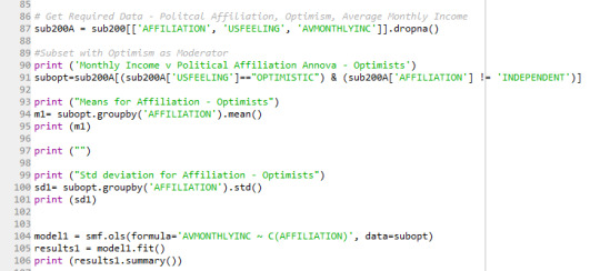
The results for Optimism shows the F statistic of 0.0531 and probability value p of 0.818 respectively. These low values demonstrate that there is no relationship between the variables and shows that the moderating variable (in this case Optimism) has no effect.

Test Two:  Pessimism as the moderating variable.

With a F value of 0.07599 and a p value of 0.783, the results show a similar outcome to the first test - a statistically insignificant chance that there is a relationship between Income and Affiliation. Again, the moderating variable (Pessimism) had no impact.

Based on these results it is still clear that no link exists between Income and Political Affiliation exists. I had thought it possible that Optimistic or Pessimistic samples would have been behaved differently, but this was not the case.

[laketofountain]

Pearson Correlations

Since the relationship between Optimism and Political Leaning (my chosen hypothesis) demonstrated by the 2012 Outlook on Life survey (Robnett, Tate) requires the comparison of categorical variables, I decided to look at some of the other variables in the survey to learn a little about the Pearson Correlation tool. 

In an earlier exercise I created a quantitative variable, Average Monthly Income (AVMONTHLYINC) which ranged from $200 - $16000. In this exercise I examined the relationships between this quantitative explanatory variable and 3 quantitative response variables (all were rated from 0 to 100). 

How participants rated undocumented aliens

How participants rated the top 1%

How participants rated public school teachers

The goal was to determine whether or not there was a relationship between a person’s income and their attitude to the demographics mentioned.

The code exert to run the scatter plots and Pearson Correlations follows

For the relationship between undocumented aliens and average monthly income the scatterplot shows that the relationship between the two variables and at first glance it seems like there is nothing to link them.

If we examine the results of the correlation (below), we see a positive correlation co-efficient  r = 0.014 and probability p = 0.709 (much higher than 0.05, the point at which we would reject the null hypothesis). 

This tells us that there statistically, a very small chance that there is a relationship between the two variables (since r is close to 0) so in this case we can assume that Income and attitude to undocumented aliens are not related.

The second test checks the relationship between average monthly income and respondent attitudes to the top 1%. 

The correlation results shown below follow a similar path to the first

In this case we see a negative linear correlation co-efficient (0.013) - and still a high probability value (0.71) suggesting again that we don’t have a relationship between the two (the closer the r  is to 0 the less chance of a relationship)

The final scatterplot shows the results for Public School Teachers

The correlation results in this case are a little different -

The output shows a positive linear correlation which is still low (r=0.09) but there may still be a relationship (p is now lower than 0.05 which would cause us to reject the notion that there is no relationship)  and the scatterplot seems to support that. However there are fewer folks in the high income ranges which would explain the frequency pattern on the graph. One thing seems clear though, the public school teacher would appear to rate well across all income levels with fewer detractors than the other two comparisons.

[laketofountain]

Bonferroni - not Famous for Pasta

This week, to supplement the Anova analysis carried out in the last exercise, I am running a Chi-Square Test of Independence Analysis on 2 categorical variables in the 2012 Outlook on Life survey (Robnett, Tate). The items in question are Political Leaning and Feeling. The Political Leaning variable (W1_C2) is a 7 level categorical explanatory variable with values from 1 (Liberal) to 7 (Conservative). The Feeling variable (USFEELING) is a 2 value response variable with the values ‘Optimistic’ and ‘Pessimistic’.

The Hypothesis is that there is a relationship between Feeling and Political Leaning and the Null Hypothesis is that there is no relationship between the two variables.

The code to run the analysis is follows:

My results are below, first frequency and then percentages.

In this case the Chi-Square value is ~105.41 and the p value is ~1.86e-20. These values suggest that Feeling and Political Leaning are related (large Chi-Square value and a p value lower than 0.005).

Since the explanatory variable is a 7 level variable it is necessary to carry out a post hoc test to determine why the results from the Chi-Square test suggest that we should reject the null hypothesis. For a multi level variable it is necessary to test each paired value in the set. The probability (p) value is adjusted to reduce the possibility of rejecting the null hypothesis using the Bonferroni Adjustment. This divides p (0.005) by the number of tests we plan to carry out (in this case, since we are comparing 7 values there are 21 tests, so 0.005/21 gives us a p value of 0.0023).

A section of the code is shown along with the outputs for the two comparisons - 1 and 2 and 1 and 3. 

Results for these comparisons:

The results of the 21 tests are summarized in the table that follows. The p values highlighted in green show where definite relationships exist between the explanatory and response variables. A complete listing of the program plus output follows the summary. Enjoy!

Program Listing:

# -*- coding: utf-8 -*- """ Spyder Editor

This is a temporary script file. """ import pandas import numpy import seaborn import matplotlib.pyplot as plt import matplotlib.patches as mpatches import statsmodels.formula.api as smf import statsmodels.stats.multicomp as multi import scipy.stats

data = pandas.read_csv('ool_pds.csv', low_memory=False)

#Set PANDAS to show all columns in DataFrame pandas.set_option('display.max_columns', None) #Set PANDAS to show all rows in DataFrame pandas.set_option('display.max_rows', None)

# bug fix for display formats to avoid run time errors pandas.set_option('display.float_format', lambda x:'%f'%x)

#convert fields of interest to numberic type #Can optimism and political affiliation be linked?

#ARE YOU OPTIMISTIC? data["W2_QE1"] = pandas.to_numeric((data["W2_QE1"]),errors='coerce') #PERSONAL BELIEF - CONSRVATIVE or LIBERAL data["W1_C2"] = pandas.to_numeric((data["W1_C2"]),errors='coerce') #HOUSE OWNERSHIP data["PPRENT"] = pandas.to_numeric((data["PPRENT"]),errors='coerce') #HOUSEHOLD INCOME data["PPINCIMP"] = pandas.to_numeric((data["PPINCIMP"]),errors='coerce') #lowercase data.columns = map(str.upper, data.columns)

#how much data is there?

print (" ") print ('Assumptions') print (" ") print ('Liberals - those with a rating of 1-3 on Scale of 1-7 where 1 is very Liberal and 7 is very Conservative') print ('Independent - those with a rating of 4 on Scale of 1-7 where 1 is very Liberal and 7 is very Conservative') print ('Conservative - those with a rating of 1-3 on Scale of 1-7 where 1 is very Liberal and 7 is very Conservative') print (" ") print (" ")

#DATA MANAGEMENT

#Create data subset #Assign Home Ownership categories - Map 1 to OWN, 2 to RENT, Exclude 3  and remove missing data for political affiliation (-1) #Include only data for optimists and pessimists

submain=data[(data['PPRENT']<3) & (data["W1_C2"]>0)] submain=submain[(submain['W2_QE1'] >= 1)] submain=submain[(submain['W2_QE1'] < 3)]

print ("Describe Political Affiliation of all Participants (missing data removed)" ) desc= submain['W2_QE1'].describe() print (desc)

#Make a copy for manipulation sub200 = submain.copy()

#Subsets for Graphing recode1 = {1: "OWN", 2: "RENT"} sub200['USROB']= sub200['PPRENT'].map(recode1) #Make Own or Rent Column 1 or 0 for Categorical Response Variable recode3 = {1: "1", 2: "0"} sub200['USROBBIN']= sub200['PPRENT'].map(recode3) #Create Categorical Response Variable for Income (Low (0-40k), Middle (41-125k), Top (>125k)) recode2 = {1: "LOW", 2: "LOW", 3: "LOW", 4: "LOW", 5: "LOW", 6: "LOW", 7: "LOW", 8: "LOW", 9: "LOW", 10: "LOW", 11: "MIDDLE", 12: "MIDDLE", 13: "MIDDLE", 14: "MIDDLE", 15: "MIDDLE", 16: "MIDDLE", 17: "TOP", 18: "TOP", 19: "TOP" } sub200['USINC']= sub200['PPINCIMP'].map(recode2) #Create Categorical Repsonse Variable for Political Affiliation (Including Ind.) recode4 = {1: "LIBERAL", 2: "LIBERAL", 3: "LIBERAL", 4: "INDEPENDENT", 5:"CONSERVATIVE", 6:"CONSERVATIVE", 7:"CONSERVATIVE"} sub200['AFFILIATION']= sub200['W1_C2'].map(recode4) #Create Categorical Repsonse Variable for Optimist and Pessimist recode5 = {1: "OPTIMISTIC", 2: "PESSIMISTIC"} sub200['USFEELING']= sub200['W2_QE1'].map(recode5)

#Create Median Monthly Income based Income bands (0-5000, 5000-7499 etc - average monthly = [Low +high / 2]/12) recode6 = {1: 208, 2: 521, 3: 729, 4: 937, 5: 1146, 6: 1458, 7: 1875, 8: 2292, 9: 2708, 10: 3125, 11: 3750, 12: 4583, 13: 5625, 14: 6667, 15: 7708, 16: 9375, 17: 11458, 18: 13452, 19: 15625 } sub200['AVMONTHLYINC']= sub200['PPINCIMP'].map(recode6)

# contingency table based on liberal - conservative leaning (7 level categorical variable) vs Optimism (bi-level)

# contingency table of observed counts print ('Pessimism vs Optimism based on Politcial Leaning (scale: 1 - Liberal to 7 - Conservative)') ct1=pandas.crosstab(sub200['USFEELING'], sub200['W1_C2']) print (ct1)

# column percentages colsum=ct1.sum(axis=0) colpct=ct1/colsum print(colpct)

# chi-square print ('chi-square value, p value, expected counts') cs1= scipy.stats.chi2_contingency(ct1) print (cs1)

#Bonferroni - 21 tests (7 variable comparisons) #pvalue - 0.0024 (0.005/21)

print ('Chi-sqaure post hoc testing using Bonferroni Adjustment') print ('') print ('************ 1 v 2 ***************')

print ('chi-square value, p value, expected counts')

recodecomp1 = {1: 1, 2: 2} sub200['COMP1v2']= sub200['W1_C2'].map(recodecomp1)

# contingency table of observed counts ct2=pandas.crosstab(sub200['USFEELING'], sub200['COMP1v2']) print (ct2)

# column percentages colsum=ct2.sum(axis=0) colpct=ct2/colsum print(colpct)

print ('chi-square value, p value, expected counts') cs2= scipy.stats.chi2_contingency(ct2) print (cs2)

print ('************ 1 v 3 ***************')

recodecomp2 = {1: 1, 3: 3} sub200['COMP1v3']= sub200['W1_C2'].map(recodecomp2)

# contingency table of observed counts ct3=pandas.crosstab(sub200['USFEELING'], sub200['COMP1v3']) print (ct3)

# column percentages colsum=ct3.sum(axis=0) colpct=ct3/colsum print(colpct)

print ('chi-square value, p value, expected counts') cs3= scipy.stats.chi2_contingency(ct3) print (cs3)

print ('************ 1 v 4 ***************')

recodecomp4 = {1: 1, 4: 4} sub200['COMP1v4']= sub200['W1_C2'].map(recodecomp4)

# contingency table of observed counts ct4=pandas.crosstab(sub200['USFEELING'], sub200['COMP1v4']) print (ct4)

# column percentages colsum=ct4.sum(axis=0) colpct=ct4/colsum print(colpct)

print ('chi-square value, p value, expected counts') cs4= scipy.stats.chi2_contingency(ct4) print (cs4)

print ('************ 1 v 5 ***************')

recodecomp5 = {1: 1, 5: 5} sub200['COMP1v5']= sub200['W1_C2'].map(recodecomp5)

# contingency table of observed counts ct5=pandas.crosstab(sub200['USFEELING'], sub200['COMP1v5']) print (ct5)

# column percentages colsum=ct5.sum(axis=0) colpct=ct5/colsum print(colpct)

print ('chi-square value, p value, expected counts') cs5= scipy.stats.chi2_contingency(ct5) print (cs5)

print ('************ 1 v 6 ***************')

recodecomp6 = {1: 1, 6: 6} sub200['COMP1v6']= sub200['W1_C2'].map(recodecomp6)

# contingency table of observed counts ct6=pandas.crosstab(sub200['USFEELING'], sub200['COMP1v6']) print (ct6)

# column percentages colsum=ct6.sum(axis=0) colpct=ct6/colsum print(colpct)

print ('chi-square value, p value, expected counts') cs6= scipy.stats.chi2_contingency(ct6) print (cs6)

print ('************ 1 v 7 ***************')

recodecomp7 = {1: 1, 7: 7} sub200['COMP1v7']= sub200['W1_C2'].map(recodecomp7)

# contingency table of observed counts ct7=pandas.crosstab(sub200['USFEELING'], sub200['COMP1v7']) print (ct7)

# column percentages colsum=ct7.sum(axis=0) colpct=ct7/colsum print(colpct)

print ('chi-square value, p value, expected counts') cs7= scipy.stats.chi2_contingency(ct7) print (cs7)

print ('************ 2 v 3 ***************')

print ('chi-square value, p value, expected counts')

recodecomp23 = {2: 2, 3: 3} sub200['COMP2v3']= sub200['W1_C2'].map(recodecomp23)

# contingency table of observed counts ct23=pandas.crosstab(sub200['USFEELING'], sub200['COMP2v3']) print (ct23)

# column percentages colsum=ct23.sum(axis=0) colpct=ct23/colsum print(colpct)

print ('chi-square value, p value, expected counts') cs23= scipy.stats.chi2_contingency(ct23) print (cs23)

print ('************ 2 v 4 ***************')

recodecomp24 = {2: 2, 4: 4} sub200['COMP2v4']= sub200['W1_C2'].map(recodecomp24)

# contingency table of observed counts ct24=pandas.crosstab(sub200['USFEELING'], sub200['COMP2v4']) print (ct24)

# column percentages colsum=ct24.sum(axis=0) colpct=ct24/colsum print(colpct)

print ('chi-square value, p value, expected counts') cs24= scipy.stats.chi2_contingency(ct4) print (cs24)

print ('************ 2 v 5 ***************')

recodecomp25 = {2: 2, 5: 5} sub200['COMP2v5']= sub200['W1_C2'].map(recodecomp25)

# contingency table of observed counts ct25=pandas.crosstab(sub200['USFEELING'], sub200['COMP2v5']) print (ct25)

# column percentages colsum=ct25.sum(axis=0) colpct=ct25/colsum print(colpct)

print ('chi-square value, p value, expected counts') cs25= scipy.stats.chi2_contingency(ct25) print (cs25)

print ('************ 2 v 6 ***************')

recodecomp26 = {2: 2, 6: 6} sub200['COMP2v6']= sub200['W1_C2'].map(recodecomp26)

# contingency table of observed counts ct26=pandas.crosstab(sub200['USFEELING'], sub200['COMP2v6']) print (ct26)

# column percentages colsum=ct26.sum(axis=0) colpct=ct26/colsum print(colpct)

print ('chi-square value, p value, expected counts') cs26= scipy.stats.chi2_contingency(ct26) print (cs26)

print ('************ 2 v 7 ***************')

recodecomp27 = {2: 2, 7: 7} sub200['COMP2v7']= sub200['W1_C2'].map(recodecomp27)

# contingency table of observed counts ct27=pandas.crosstab(sub200['USFEELING'], sub200['COMP2v7']) print (ct27)

# column percentages colsum=ct27.sum(axis=0) colpct=ct27/colsum print(colpct)

print ('chi-square value, p value, expected counts') cs27= scipy.stats.chi2_contingency(ct27) print (cs27)

print ('************ 3 v 4 ***************')

recodecomp34 = {3: 3, 4: 4} sub200['COMP3v4']= sub200['W1_C2'].map(recodecomp34)

# contingency table of observed counts ct34=pandas.crosstab(sub200['USFEELING'], sub200['COMP3v4']) print (ct34)

# column percentages colsum=ct34.sum(axis=0) colpct=ct34/colsum print(colpct)

print ('chi-square value, p value, expected counts') cs34= scipy.stats.chi2_contingency(ct34) print (cs34)

print ('************ 3 v 5 ***************')

recodecomp35 = {3: 3, 5: 5} sub200['COMP3v5']= sub200['W1_C2'].map(recodecomp35)

# contingency table of observed counts ct35=pandas.crosstab(sub200['USFEELING'], sub200['COMP3v5']) print (ct35)

# column percentages colsum=ct35.sum(axis=0) colpct=ct35/colsum print(colpct)

print ('chi-square value, p value, expected counts') cs35= scipy.stats.chi2_contingency(ct35) print (cs35)

print ('************ 3 v 6 ***************')

recodecomp36 = {3: 3, 6: 6} sub200['COMP3v6']= sub200['W1_C2'].map(recodecomp36)

# contingency table of observed counts ct36=pandas.crosstab(sub200['USFEELING'], sub200['COMP3v6']) print (ct36)

# column percentages colsum=ct36.sum(axis=0) colpct=ct36/colsum print(colpct)

print ('chi-square value, p value, expected counts') cs36= scipy.stats.chi2_contingency(ct36) print (cs36)

print ('************ 3 v 7 ***************')

recodecomp37 = {3: 3, 7: 7} sub200['COMP3v7']= sub200['W1_C2'].map(recodecomp37)

# contingency table of observed counts ct37=pandas.crosstab(sub200['USFEELING'], sub200['COMP3v7']) print (ct37)

# column percentages colsum=ct37.sum(axis=0) colpct=ct37/colsum print(colpct)

print ('chi-square value, p value, expected counts') cs37= scipy.stats.chi2_contingency(ct37) print (cs37)

print ('************ 4 v 5 ***************')

recodecomp45 = {4: 4, 5: 5} sub200['COMP4v5']= sub200['W1_C2'].map(recodecomp45)

# contingency table of observed counts ct45=pandas.crosstab(sub200['USFEELING'], sub200['COMP4v5']) print (ct45)

# column percentages colsum=ct45.sum(axis=0) colpct=ct45/colsum print(colpct)

print ('chi-square value, p value, expected counts') cs45= scipy.stats.chi2_contingency(ct45) print (cs45)

print ('************ 4 v 6 ***************')

recodecomp46 = {4: 4, 6: 6} sub200['COMP4v6']= sub200['W1_C2'].map(recodecomp46)

# contingency table of observed counts ct46=pandas.crosstab(sub200['USFEELING'], sub200['COMP4v6']) print (ct46)

# column percentages colsum=ct46.sum(axis=0) colpct=ct46/colsum print(colpct)

print ('chi-square value, p value, expected counts') cs46= scipy.stats.chi2_contingency(ct46) print (cs46)

print ('************ 4 v 7 ***************')

recodecomp47 = {4: 4, 7: 7} sub200['COMP4v7']= sub200['W1_C2'].map(recodecomp47)

# contingency table of observed counts ct47=pandas.crosstab(sub200['USFEELING'], sub200['COMP4v7']) print (ct47)

# column percentages colsum=ct47.sum(axis=0) colpct=ct47/colsum print(colpct)

print ('chi-square value, p value, expected counts') cs47= scipy.stats.chi2_contingency(ct47) print (cs47)

print ('************ 5 v 6 ***************')

recodecomp56 = {5: 5, 6: 6} sub200['COMP5v6']= sub200['W1_C2'].map(recodecomp56)

# contingency table of observed counts ct56=pandas.crosstab(sub200['USFEELING'], sub200['COMP5v6']) print (ct56)

# column percentages colsum=ct56.sum(axis=0) colpct=ct56/colsum print(colpct)

print ('chi-square value, p value, expected counts') cs56= scipy.stats.chi2_contingency(ct56) print (cs56)

print ('************ 5 v 7 ***************')

recodecomp57 = {5: 5, 7: 7} sub200['COMP5v7']= sub200['W1_C2'].map(recodecomp57)

# contingency table of observed counts ct57=pandas.crosstab(sub200['USFEELING'], sub200['COMP5v7']) print (ct57)

# column percentages colsum=ct57.sum(axis=0) colpct=ct57/colsum print(colpct)

print ('chi-square value, p value, expected counts') cs57= scipy.stats.chi2_contingency(ct57) print (cs57)

print ('************ 6 v 7 ***************')

recodecomp67 = {6: 6, 7: 7} sub200['COMP6v7']= sub200['W1_C2'].map(recodecomp67)

# contingency table of observed counts ct67=pandas.crosstab(sub200['USFEELING'], sub200['COMP6v7']) print (ct67)

# column percentages colsum=ct67.sum(axis=0) colpct=ct67/colsum print(colpct)

print ('chi-square value, p value, expected counts') cs67= scipy.stats.chi2_contingency(ct67) print (cs67)

Output:

Assumptions

Liberals - those with a rating of 1-3 on Scale of 1-7 where 1 is very Liberal and 7 is very Conservative Independent - those with a rating of 4 on Scale of 1-7 where 1 is very Liberal and 7 is very Conservative Conservative - those with a rating of 1-3 on Scale of 1-7 where 1 is very Liberal and 7 is very Conservative

Describe Political Affiliation of all Participants (missing data removed) count   1074.000000 mean       1.206704 std        0.405130 min        1.000000 25%        1.000000 50%        1.000000 75%        1.000000 max        2.000000 Name: W2_QE1, dtype: float64 Pessimism vs Optimism based on Politcial Leaning (scale: 1 - Liberal to 7 - Conservative) W1_C2         1    2    3    4    5    6   7 USFEELING                                   OPTIMISTIC   27  145  138  314  105  103  20 PESSIMISTIC   5   10   20   55   40   69  23 W1_C2              1        2        3        4        5        6        7 USFEELING                                                                 OPTIMISTIC  0.843750 0.935484 0.873418 0.850949 0.724138 0.598837 0.465116 PESSIMISTIC 0.156250 0.064516 0.126582 0.149051 0.275862 0.401163 0.534884 chi-square value, p value, expected counts (105.40880123421682, 1.8617010557256508e-20, 6, array([[  25.38547486,  122.96089385,  125.34078212,  292.72625698,         115.02793296,  136.44692737,   34.11173184],       [   6.61452514,   32.03910615,   32.65921788,   76.27374302,          29.97206704,   35.55307263,    8.88826816]])) Chi-sqaure post hoc testing using Bonferroni Adjustment

************ 1 v 2 *************** chi-square value, p value, expected counts COMP1v2      1.000000  2.000000 USFEELING                       OPTIMISTIC         27       145 PESSIMISTIC         5        10 COMP1v2      1.000000  2.000000 USFEELING                       OPTIMISTIC   0.843750  0.935484 PESSIMISTIC  0.156250  0.064516 chi-square value, p value, expected counts (1.9096634119467368, 0.16700065219498123, 1, array([[  29.43315508,  142.56684492],       [   2.56684492,   12.43315508]])) ************ 1 v 3 *************** COMP1v3      1.000000  3.000000 USFEELING                       OPTIMISTIC         27       138 PESSIMISTIC         5        20 COMP1v3      1.000000  3.000000 USFEELING                       OPTIMISTIC   0.843750  0.873418 PESSIMISTIC  0.156250  0.126582 chi-square value, p value, expected counts (0.02755801687763719, 0.8681521694924621, 1, array([[  27.78947368,  137.21052632],       [   4.21052632,   20.78947368]])) ************ 1 v 4 *************** COMP1v4      1.000000  4.000000 USFEELING                       OPTIMISTIC         27       314 PESSIMISTIC         5        55 COMP1v4      1.000000  4.000000 USFEELING                       OPTIMISTIC   0.843750  0.850949 PESSIMISTIC  0.156250  0.149051 chi-square value, p value, expected counts (0.02214248541174926, 0.88170867871508918, 1, array([[  27.21197007,  313.78802993],       [   4.78802993,   55.21197007]])) ************ 1 v 5 *************** COMP1v5      1.000000  5.000000 USFEELING                       OPTIMISTIC         27       105 PESSIMISTIC         5        40 COMP1v5      1.000000  5.000000 USFEELING                       OPTIMISTIC   0.843750  0.724138 PESSIMISTIC  0.156250  0.275862 chi-square value, p value, expected counts (1.3975653898902822, 0.23713162935968868, 1, array([[  23.86440678,  108.13559322],       [   8.13559322,   36.86440678]])) ************ 1 v 6 *************** COMP1v6      1.000000  6.000000 USFEELING                       OPTIMISTIC         27       103 PESSIMISTIC         5        69 COMP1v6      1.000000  6.000000 USFEELING                       OPTIMISTIC   0.843750  0.598837 PESSIMISTIC  0.156250  0.401163 chi-square value, p value, expected counts (5.9815364671469338, 0.014456402869507837, 1, array([[  20.39215686,  109.60784314],       [  11.60784314,   62.39215686]])) ************ 1 v 7 *************** COMP1v7      1.000000  7.000000 USFEELING                       OPTIMISTIC         27        20 PESSIMISTIC         5        23 COMP1v7      1.000000  7.000000 USFEELING                       OPTIMISTIC   0.843750  0.465116 PESSIMISTIC  0.156250  0.534884 chi-square value, p value, expected counts (9.6823303692920746, 0.0018604850982736709, 1, array([[ 20.05333333,  26.94666667],       [ 11.94666667,  16.05333333]])) ************ 2 v 3 *************** chi-square value, p value, expected counts COMP2v3      2.000000  3.000000 USFEELING                       OPTIMISTIC        145       138 PESSIMISTIC        10        20 COMP2v3      2.000000  3.000000 USFEELING                       OPTIMISTIC   0.935484  0.873418 PESSIMISTIC  0.064516  0.126582 chi-square value, p value, expected counts (2.7987115928185866, 0.094340088093986238, 1, array([[ 140.14376997,  142.85623003],       [  14.85623003,   15.14376997]])) ************ 2 v 4 *************** COMP2v4      2.000000  4.000000 USFEELING                       OPTIMISTIC        145       314 PESSIMISTIC        10        55 COMP2v4      2.000000  4.000000 USFEELING                       OPTIMISTIC   0.935484  0.850949 PESSIMISTIC  0.064516  0.149051 chi-square value, p value, expected counts (0.02214248541174926, 0.88170867871508918, 1, array([[  27.21197007,  313.78802993],       [   4.78802993,   55.21197007]])) ************ 2 v 5 *************** COMP2v5      2.000000  5.000000 USFEELING                       OPTIMISTIC        145       105 PESSIMISTIC        10        40 COMP2v5      2.000000  5.000000 USFEELING                       OPTIMISTIC   0.935484  0.724138 PESSIMISTIC  0.064516  0.275862 chi-square value, p value, expected counts (22.595773081201337, 1.9992397734327818e-06, 1, array([[ 129.16666667,  120.83333333],       [  25.83333333,   24.16666667]])) ************ 2 v 6 *************** COMP2v6      2.000000  6.000000 USFEELING                       OPTIMISTIC        145       103 PESSIMISTIC        10        69 COMP2v6      2.000000  6.000000 USFEELING                       OPTIMISTIC   0.935484  0.598837 PESSIMISTIC  0.064516  0.401163 chi-square value, p value, expected counts (48.608086674364841, 3.1257767670735383e-12, 1, array([[ 117.55351682,  130.44648318],       [  37.44648318,   41.55351682]])) ************ 2 v 7 *************** COMP2v7      2.000000  7.000000 USFEELING                       OPTIMISTIC        145        20 PESSIMISTIC        10        23 COMP2v7      2.000000  7.000000 USFEELING                       OPTIMISTIC   0.935484  0.465116 PESSIMISTIC  0.064516  0.534884 chi-square value, p value, expected counts (50.288732183045759, 1.3270935741868568e-12, 1, array([[ 129.16666667,   35.83333333],       [  25.83333333,    7.16666667]])) ************ 3 v 4 *************** COMP3v4      3.000000  4.000000 USFEELING                       OPTIMISTIC        138       314 PESSIMISTIC        20        55 COMP3v4      3.000000  4.000000 USFEELING                       OPTIMISTIC   0.873418  0.850949 PESSIMISTIC  0.126582  0.149051 chi-square value, p value, expected counts (0.29201551688092608, 0.58893182535690092, 1, array([[ 135.5142315,  316.4857685],       [  22.4857685,   52.5142315]])) ************ 3 v 5 *************** COMP3v5      3.000000  5.000000 USFEELING                       OPTIMISTIC        138       105 PESSIMISTIC        20        40 COMP3v5      3.000000  5.000000 USFEELING                       OPTIMISTIC   0.873418  0.724138 PESSIMISTIC  0.126582  0.275862 chi-square value, p value, expected counts (9.6907411651066173, 0.00185198823181632, 1, array([[ 126.71287129,  116.28712871],       [  31.28712871,   28.71287129]])) ************ 3 v 6 *************** COMP3v6      3.000000  6.000000 USFEELING                       OPTIMISTIC        138       103 PESSIMISTIC        20        69 COMP3v6      3.000000  6.000000 USFEELING                       OPTIMISTIC   0.873418  0.598837 PESSIMISTIC  0.126582  0.401163 chi-square value, p value, expected counts (30.144636362671896, 4.0099467430317328e-08, 1, array([[ 115.38787879,  125.61212121],       [  42.61212121,   46.38787879]])) ************ 3 v 7 *************** COMP3v7      3.000000  7.000000 USFEELING                       OPTIMISTIC        138        20 PESSIMISTIC        20        23 COMP3v7      3.000000  7.000000 USFEELING                       OPTIMISTIC   0.873418  0.465116 PESSIMISTIC  0.126582  0.534884 chi-square value, p value, expected counts (31.124712549835955, 2.4197110638053693e-08, 1, array([[ 124.19900498,   33.80099502],       [  33.80099502,    9.19900498]])) ************ 4 v 5 *************** COMP4v5      4.000000  5.000000 USFEELING                       OPTIMISTIC        314       105 PESSIMISTIC        55        40 COMP4v5      4.000000  5.000000 USFEELING                       OPTIMISTIC   0.850949  0.724138 PESSIMISTIC  0.149051  0.275862 chi-square value, p value, expected counts (10.284694927299604, 0.0013413819611359889, 1, array([[ 300.79961089,  118.20038911],       [  68.20038911,   26.79961089]])) ************ 4 v 6 *************** COMP4v6      4.000000  6.000000 USFEELING                       OPTIMISTIC        314       103 PESSIMISTIC        55        69 COMP4v6      4.000000  6.000000 USFEELING                       OPTIMISTIC   0.850949  0.598837 PESSIMISTIC  0.149051  0.401163 chi-square value, p value, expected counts (40.791508488770077, 1.6936744025960089e-10, 1, array([[ 284.4232902,  132.5767098],       [  84.5767098,   39.4232902]])) ************ 4 v 7 *************** COMP4v7      4.000000  7.000000 USFEELING                       OPTIMISTIC        314        20 PESSIMISTIC        55        23 COMP4v7      4.000000  7.000000 USFEELING                       OPTIMISTIC   0.850949  0.465116 PESSIMISTIC  0.149051  0.534884 chi-square value, p value, expected counts (34.883307428513099, 3.500693287658955e-09, 1, array([[ 299.1407767,   34.8592233],       [  69.8592233,    8.1407767]])) ************ 5 v 6 *************** COMP5v6      5.000000  6.000000 USFEELING                       OPTIMISTIC        105       103 PESSIMISTIC        40        69 COMP5v6      5.000000  6.000000 USFEELING                       OPTIMISTIC   0.724138  0.598837 PESSIMISTIC  0.275862  0.401163 chi-square value, p value, expected counts (4.9335744411322526, 0.026339780455611996, 1, array([[  95.14195584,  112.85804416],       [  49.85804416,   59.14195584]])) ************ 5 v 7 *************** COMP5v7      5.000000  7.000000 USFEELING                       OPTIMISTIC        105        20 PESSIMISTIC        40        23 COMP5v7      5.000000  7.000000 USFEELING                       OPTIMISTIC   0.724138  0.465116 PESSIMISTIC  0.275862  0.534884 chi-square value, p value, expected counts (8.8578690800779025, 0.0029182805497870072, 1, array([[ 96.40957447,  28.59042553],       [ 48.59042553,  14.40957447]])) ************ 6 v 7 *************** COMP6v7      6.000000  7.000000 USFEELING                       OPTIMISTIC        103        20 PESSIMISTIC        69        23 COMP6v7      6.000000  7.000000 USFEELING                       OPTIMISTIC   0.598837  0.465116 PESSIMISTIC  0.401163  0.534884 chi-square value, p value, expected counts (1.9961503623188408, 0.15769928782411674, 1, array([[ 98.4,  24.6],       [ 73.6,  18.4]]))

[laketofountain]

Super Anova

Testing with more than a hunch

Onto subject two in this journey - Data Analysis Tools. 

In my last post I examined the relationship between Optimism and Political Affiliation. Based on the modeling output built using Python (and the associated graphs) it would appear that there is a relationship. As it turns out the word ‘appear’ is accurate. There is was no substantive test, just a theory based on the graphical output. A hunch, basically. So now its time to see if I can prove the hypothesis (or reject the null hypothesis). Note The working data set is the 2012 Outlook on Life Survey (Robnett / Tate) with a sample of people who claimed either to be optimistic or pessimistic about their future.

To learn how to test my hypothesis I started with an Anova that explores the relationship between between a person’s Average Monthly Income (quantitative variable) and their frame of mind - a 2 level categorical variable with the values Optimistic or Pessimistic. The sample size was 1074.

Monthly income was extrapolated from a 19 band categorical variable (income bands) to average monthly income values as follows - I took the lower band value, added it to the upper band value and divided it by two for the mean for that band. I then divided the result by 12 to give the monthly average. For example, for the category $85,000 - $99,999 I summed the lower and upper values and divided them by 2 to get a mean of $92,500 and then divided by 12 to get an average monthly income of $7708. For the upper band, > $175k I used $200k as the upper delimiter. The code except is shown below. 

The results for this Anova are as follows

The F Statistic 1.389 and the p value is 0.239 which is much greater than the p value at which we would reject the null hypothesis (>0.05). Based on these results we can say that there is no relationship between income and state of mind. Maybe money doesn't buy happiness!

To follow, I ran Anova examining a multi value categorical value, exploring the relationship between average monthly income and ethnicity.

 The Anova results for this are shown

We can see here that the F-statistic is 4.754 with a p value of 0.00835 - lower than p 0.05. This suggests that we can reject the null hypothesis that there is no relationship between monthly income and ethnicity. However it doesn't explain why. 

The code for ethnicity follows

1 White, Non-Hispanic  2 Black, Non-Hispanic  3 Other, Non-Hispanic  4 Hispanic  5 2+ Races, Non-Hispanic

To understand what is driving the result I ran a Tukey post hoc test to compare the 5 groups to each other and understand which comparison(s) will result in the rejection of the null hypothesis. 

The test shows a difference between group 1 (white) and group 2 (black). Based on these results we can reject the null hypothesis and establish that there is a relationship between ethnicity and average monthly income when comparing white and black ethnicity categories.

[laketofountain]

Making Sense of the Data

Here I am at week 4 in the journey from the lake to the mountain. I have been trying to determine whether or not there is a link between political affiliation and optimism based on the 2012 Outlook On Life survey. The results so far have been interesting and the opportunity to graphically analyse the data has been especially helpful in my quest to prove whether or not a relationship exists.

To assist with explaining my results I will include the graphical output from my exercise with the program listing and complete output to follow. It is worth noting that the data is categorical so the charts chosen to highlight the data are bar charts. 

Step 1: To start, I graphed the distribution of political affiliation - it is based on a sample size of 1074 responses - those people who described themselves as optimistic or pessimistic (there were values for those who described themselves as neither or who did not respond, both of which were removed). The distribution in Uni-modal and is evenly distributed. 

As you can see, most folks (the distribution mode and mean in this case) fall into the middle (Independent) and the distribution is almost identical for those on either side of the mode. You might be interested to know that my precinct in Wake County, NC aligns with this pattern (assuming that folks in categories 1-3 register with the Democratic Party and 5-7 with the Republican Party) - we have 1500 registered Democrats, 3000 Unaffiliated and 1500 registered Republicans

The other uni-modal variables were Optimism / Pessimism with most responses falling into the Optimistic category in our Sample and the Income Level variable where most respondents would be considered middle income.

Step 2: Next was to align Income levels (see my last post to understand how I categorized them) with affiliation to see if there was a relationship between those two variables. There are 3 distributions included in the chart below - Low Income, Middle Income and High Income. All 3 are bi-variate comparing the explanatory variable - Affiliation to the response variable - Income to answer the question “Does Income impact political affiliation?”

The distribution is uniform across all income levels and almost matches the initial distribution for Affiliation in all 3 income categories ( with the exception of a spike for the Middle Income distribution (green) on the Conservative half of the distribution. The Income vs Affiliation distribution is Uni-modal for Low and Top income respondents but could be considered bi-modal in the case of the Middle Income variable. 

Since Income followed the same distribution pattern across the Affiliation spectrum it was eliminated as a factor in the relationship between Optimism and Political Affiliation. There is further supporting data on this in program output as I a applied the same tests to each income level individually. Since they followed the same pattern the conclusion did not change (see the graphs in the program output that follows).

Step 3: I applied the Optimism variable to affiliation.

This distribution applies the optimism / pessimism variable to the analysis creating 2 bi-variate distributions. Interestingly, while the optimism measure follows a similar pattern to the initial affiliation distribution in step 1, the pessimism distribution is skewed left demonstrating that as we move to the right in the political spectrum, there does indeed seem to be an increase in pessimism.

The initial hypotheses (”Are Liberals more Optimistic than Conservatives?”) would seem at first glance to be proven, however, there are many factors that may affect the data and the mood of those interviewed. This was before the 2012 election so it is possible that the feelings affected by that election also skewed the results somewhat. It would be interesting to revisit the models with data from the 2016 survey. 

Program Listing

# -*- coding: utf-8 -*-

"""

Spyder Editor

This is a temporary script file.

"""

import pandas 

import numpy

import seaborn

import matplotlib.pyplot as plt

import matplotlib.patches as mpatches

data = pandas.read_csv('ool_pds.csv', low_memory=False)

#Set PANDAS to show all columns in DataFrame

pandas.set_option('display.max_columns', None)

#Set PANDAS to show all rows in DataFrame

pandas.set_option('display.max_rows', None)

# bug fix for display formats to avoid run time errors

pandas.set_option('display.float_format', lambda x:'%f'%x)

#convert fields of interest to numberic type

#Can optimism and political affiliation be linked?

#ARE YOU OPTIMISTIC?

data["W2_QE1"] = pandas.to_numeric((data["W2_QE1"]),errors='coerce')

#PERSONAL BELIEF - CONSRVATIVE or LIBERAL

data["W1_C2"] = pandas.to_numeric((data["W1_C2"]),errors='coerce')

#HOUSE OWNERSHIP

data["PPRENT"] = pandas.to_numeric((data["PPRENT"]),errors='coerce')

#HOUSEHOLD INCOME

data["PPINCIMP"] = pandas.to_numeric((data["PPINCIMP"]),errors='coerce')

#lowercase

data.columns = map(str.upper, data.columns)

#how much data is there?

print (" ")

print ('Assumptions')

print (" ")

print ('Liberals - those with a rating of 1-3 on Scale of 1-7 where 1 is very Liberal and 7 is very Conservative')

print ('Independant - those with a rating of 4 on Scale of 1-7 where 1 is very Liberal and 7 is very Conservative')

print ('Conservative - those with a rating of 1-3 on Scale of 1-7 where 1 is very Liberal and 7 is very Conservative')

print (" ")

print (" ")

#DATA MANAGEMENT 

#Create data subset

#Assign Home Ownership categories - Map 1 to OWN, 2 to RENT, Exclude 3  and remove missing data for political affiliation (-1)

#Include only data for optimists and pessimists

submain=data[(data['PPRENT']<3) & (data["W1_C2"]>0)]

submain=submain[(submain['W2_QE1'] >= 1)] 

submain=submain[(submain['W2_QE1'] < 3)] 

print ("Describe Political Affiliation of all Participants (missing data removed)" )

desc= submain['W2_QE1'].describe()

print (desc)

#Make a copy for manipulation

sub200 = submain.copy()

#Subsets for Graphing

recode1 = {1: "OWN", 2: "RENT"}

sub200['USROB']= sub200['PPRENT'].map(recode1)

#Make Own or Rent Column 1 or 0 for Categorical Response Variable

recode3 = {1: "1", 2: "0"}

sub200['USROBBIN']= sub200['PPRENT'].map(recode3)

#Create Categorical Response Variable for Income (Low (0-40k), Middle (41-125k), Top (>125k)) 

recode2 = {1: "LOW", 2: "LOW", 3: "LOW", 4: "LOW", 5: "LOW", 6: "LOW", 7: "LOW", 8: "LOW", 9: "LOW", 10: "LOW", 11: "MIDDLE", 12: "MIDDLE", 13: "MIDDLE", 14: "MIDDLE", 15: "MIDDLE", 16: "MIDDLE", 17: "TOP", 18: "TOP", 19: "TOP" }

sub200['USINC']= sub200['PPINCIMP'].map(recode2)

#Create Categorical Repsonse Variable for Political Affiliation (Including Ind.)

recode4 = {1: "LIBERAL", 2: "LIBERAL", 3: "LIBERAL", 4: "INDEPENDENT", 5:"CONSERVATIVE", 6:"CONSERVATIVE", 7:"CONSERVATIVE"}

sub200['AFFILIATION']= sub200['W1_C2'].map(recode4)

#Create Categorical Repsonse Variable for Optimist and Pessimist

recode5 = {1: "OPTIMISTIC", 2: "PESSIMISTIC"}

sub200['USFEELING']= sub200['W2_QE1'].map(recode5)

#GRAPHING

#Univariate Variable Plots - Affiliation, Optimism and Income Level

plt.figure()

seaborn.set(style="whitegrid")

sub200['W1_C2']=sub200['W1_C2'].astype('category')

seaborn.countplot(x='W1_C2', data=sub200)

plt.xlabel('Affiliation (1 Liberal - 7 Conservative)')

plt.title('Political Affiliation Variable - Out Look on Life (OLL) Survey 2012')

plt.figure()

seaborn.set(style="whitegrid")

seaborn.countplot(x='USFEELING', data=sub200, color="b")

plt.xlabel('Optimistic vs Pessimistic')

plt.title('Optimism / Pessimism Variable - OLL Survey 2012')

plt.figure()

seaborn.set(style="whitegrid")

seaborn.countplot(x='USINC', data=sub200, order= ["LOW","MIDDLE","TOP"])

plt.xlabel('Income Groups')

plt.ylabel('Response Count')

plt.title('Income Level Variable - OOL Survey 2012')

plt.figure()

seaborn.set(style="whitegrid")

sub200['W1_C2']=sub200['W1_C2'].astype('category')

seaborn.countplot(x='W1_C2',hue='USFEELING', data=sub200, color="b")

plt.xlabel('Affiliation (1 Liberal - 7 Conservative)')

plt.title('Political Affiliation by Optimism / Pessimism - OLL Survey 2012')

plt.figure()

seaborn.set(style="whitegrid")

sub200['W1_C2']=sub200['W1_C2'].astype('category')

seaborn.countplot(x='W1_C2',hue='USINC', data=sub200, hue_order= ["LOW","MIDDLE","TOP"])

plt.xlabel('Affiliation (1 Liberal - 7 Conservative)')

plt.ylabel('Response Count')

plt.title('Political Affiliation - by Income Level - OOL Survey 2012')

sub201=sub200[(sub200['USINC']=="LOW")]

sub202=sub200[(sub200['USINC']=="MIDDLE")]

sub203=sub200[(sub200['USINC']=="TOP")]

sub204=sub201[(sub201['USFEELING']=="OPTIMISTIC")]

sub206=sub202[(sub202['USFEELING']=="OPTIMISTIC")]

sub208=sub203[(sub203['USFEELING']=="OPTIMISTIC")]

print ('Low Income Sample Description')

desc1 = sub201['USINC'].describe()

print (desc1)

print ('Middle Income Sample Description')

desc2 = sub202['USINC'].describe()

print (desc2)

print ('High Income Sample Description')

desc3 = sub203['USINC'].describe()

print (desc3)

print ('Low Income Optimist Sample Description')

desc4 = sub204['USINC'].describe()

print (desc1)

print ('Middle Income Optimist Sample Description')

desc5 = sub206['USINC'].describe()

print (desc2)

print ('High Income Optimist Sample Description')

desc6 = sub208['USINC'].describe()

print (desc3)

#Bivariate Variable Plot - Affiliation

#Low Income vs Optimism vs Affiliation

plt.figure()

seaborn.set(style="whitegrid")

sub201['W1_C2']=sub201['W1_C2'].astype('category')

seaborn.countplot(x='W1_C2',hue='USINC', data=sub201)

plt.xlabel('Affiliation (1 Liberal - 7 Conservative)')

plt.ylabel('Response Count')

plt.title('Political Affiliation / Optimism - Out Look on Life Survey 2012 - Low Income')

seaborn.countplot(data=sub204, x='W1_C2', hue="USFEELING", color="blue")

plt.xlabel('Affiliation (1 Liberal - 7 Conservative)')

plt.ylabel('Response Count')

Legend = mpatches.Patch(color='steelblue', label='Total Observations')

Legend2 = mpatches.Patch(color='gainsboro', label='Optimistic Observations')

plt.legend(handles=[Legend,Legend2])

#Middle Income vs Optimism vs Affiliation

plt.figure()

seaborn.set(style="whitegrid")

sub202['W1_C2']=sub202['W1_C2'].astype('category')

seaborn.countplot(x='W1_C2',hue='USINC', data=sub202)

plt.xlabel('Affiliation (1 Liberal - 7 Conservative)')

plt.ylabel('Response Count')

plt.title('Political Affiliation - Out Look on Life Survey 2012 - Middle Income')

seaborn.countplot(data=sub206, x='W1_C2', hue="USFEELING", color="blue")

plt.xlabel('Affiliation (1 Liberal - 7 Conservative)')

plt.ylabel('Response Count')

Legend = mpatches.Patch(color='steelblue', label='Total Observations')

Legend2 = mpatches.Patch(color='gainsboro', label='Optimistic Observations')

plt.legend(handles=[Legend,Legend2])

#Top income vs Optimism vs Affiliation

plt.figure()

seaborn.set(style="whitegrid")

sub203['W1_C2']=sub203['W1_C2'].astype('category')

seaborn.countplot(x='W1_C2',hue='USINC', data=sub203)

plt.title('Political Affiliation - Out Look on Life Survey 2012 - Top Income')

seaborn.countplot(data=sub208, x='W1_C2', hue="USFEELING", color="blue")

plt.xlabel('Affiliation (1 Liberal - 7 Conservative)')

plt.ylabel('Response Count')

Legend = mpatches.Patch(color='steelblue', label='Total Observations')

Legend2 = mpatches.Patch(color='gainsboro', label='Optimistic Observations')

plt.legend(handles=[Legend,Legend2])

Program Output











[laketofountain]

Understanding the Data

Decoding the code book and working out the Python’s quirks

This week I stumbled into the nuances of Python versions as I felt my way through the next exercise - in my last post I mentioned that I was having problems with the deprecated function convert_objects - well one week and many hours later I was able to convert using the to_numeric function. I was also able to order by index, something else that stumped me last week. See my program or ping me if you would like to learn more!

For this exercise I worked on reducing the data and trying to dig further into my hypothesis regarding whether or not Optimism and Political Affiliation are linked. The overall data would suggest that there is a link - 58% of Liberals were optimistic compared with 42% of Conservatives (see my last post). 

To try and understand what was driving these results I studied two denominators - Income and Home Ownership to see if personal wealth was a factor. I used the middle income survey by the Pew Research center (reference: America’s Shrinking Middle Class:  A Close Look at Changes Within Metropolitan Areas - Pew Research Center, May 2016) (see link) to determine my income classifications and then mapped the survey values from the Outlook on Life Surveys, 2012 (Robnett, Tate, 2012) for PPINCIMP: Household Income to those classifications, creating a new column USINC. This reduced the household income categories from 19 to 3 grouping them by Low, Middle, Top categories which was helpful when trying to gain insight to these data sets.  

Also recoded was the PPRENT: Ownership Status of Living Quarters column where I added a column USROB converting the index values from 1 to Own and 2 to Rent. I removed the value 3 which represented Neither as it was not relevant to this study. This made the readout more meaningful.

The output contains the overall results as presented in my last posting as well as some further information around the relationship between affiliation, optimism and personal wealth. You can see that the missing or unnecessary data resulted in the removal of 62 replies (those that neither owned nor rented their homes). Further reductions were made based on affiliation and optimism.

Overall Results - Output Summary (Full Readout Follows Program)

Number of Responses:                    2294 Missing and N/A responses removed:      62 Total Population:                       2232 Totals after data reduced and classified ============================================================

Total Number of Home Owners:          781 Total Number of Home Renters:         1451 Low Income Earners (<$45k):           931 Middle Income Earners(>$45k <125k:)   1030 Top Income Earners:(>$125k)           271

Data Point                        Count Distribution ==========                        ===== ============

Total who are Optimistic:           538 76.0 % Total who are Pessimistic:          167 24.0 %

Affiliation Populations

Total Number of People:             705 100 % Total lean Liberal                  345 49.0 % Total lean Conservative:            360 51.0 %

Total Number of Optimists:          538 100 % Liberals who are Optimistic:        310 58.0 % Conservatives who are Optimistic:   228 42.0 %

Total Number of Pessimists:         167 100 % Liberals who are Pessimistic:       35 21.0 % Conservatives who are Pessimistic:  132 79.0 %

Optimists who are Liberal Split by Home Ownership % OWN     67.0 RENT    33.0

Optimists who are Conservative Split by Home Ownership % OWN     71.0 RENT    29.0

Optimists who are Liberal Split by Income Distribution (Low, Middle, High) % LOW       32.0 MIDDLE    53.0 TOP       15.0

Optimists who are Conservative Split by Income Distribution (Low, Middle, High) % LOW       38.0 MIDDLE    43.0 TOP       19.0

Interestingly - the optimism distributions across these classifications are quite similar which suggests that optimism and personal wealth are likely related. However, since there are fewer optimists on the Conservative side the data would seem to still lean towards a link between Optimism and Political affiliation in general.

Total Number of Optimists:          538 100 % Liberals who are Optimistic:        310 58.0 % Conservatives who are Optimistic:   228 42.0 %

The full results can be seen in my program output. Enjoy! 

Program

# -*- coding: utf-8 -*- """ Spyder Editor

This is a temporary script file. """ import pandas import numpy

data = pandas.read_csv('ool_pds.csv', low_memory=False)

#convert fields of interest to numberic type #Can optimism and political affiliation be linked?

#ARE YOU OPTIMISTIC? data["W2_QE1"] = pandas.to_numeric((data["W2_QE1"]),errors='coerce') #PERSONAL BELIEF - CONSRVATIVE or LIBERAL data["W1_C2"] = pandas.to_numeric((data["W1_C2"]),errors='coerce') #HOUSE OWNERSHIP data["PPRENT"] = pandas.to_numeric((data["PPRENT"]),errors='coerce') #HOUSEHOLD INCOME data["PPINCIMP"] = pandas.to_numeric((data["PPINCIMP"]),errors='coerce') #lowercase data.columns = map(str.upper, data.columns)

#how much data is there?

print (" ") print ('Assumptions') print (" ") print ('Liberals - those with a rating of 1-3 on Scale of 1-7 where 1 is very Liberal and 7 is very Conservative') print ('Conservative - those with a rating of 1-3 on Scale of 1-7 where 1 is very Liberal and 7 is very Conservative') print (" ") print (" ")

#Underlying distributions print (" ") print ("Underlying Distributions:") print (" ") print ('Optimist (1), Pessimist (2), Neither (3)') #sort index used to order value counts by value c99 = data["W2_QE1"].value_counts(sort=True) c99 = c99.sort_index(ascending=True) p99 = data["W2_QE1"].value_counts(sort=False,normalize=True) p99 = p99.sort_index(ascending=True)

print (c99) print (p99)

print ('Liberal (1) to Conservative (7)') #sort index used to order value counts by value c100 = data["W1_C2"].value_counts(sort=False) c100 = c100.sort_index(ascending=True) p100 = data["W1_C2"].value_counts(sort=False, normalize=True) p100 = p100.sort_index(ascending=True) #p100r = round(p100) print (c100) print (p100) #print (((p100r)*100),"%")

print ('Sample Home Ownership (1-own, 2-rent, 3-neither)') #sort index used to order value counts by value c101 = data["PPRENT"].value_counts(sort=False) c101 = c101.sort_index(ascending=True) p101 = data["PPRENT"].value_counts(sort=False, normalize=True) p101 = p101.sort_index(ascending=True) print (c101) print (p101)

print ('Sample Income') #sort index used to order value counts by value c102 = data["PPINCIMP"].value_counts(sort=False) c102 = c102.sort_index(ascending=True) p102 = data["PPINCIMP"].value_counts(sort=False, normalize=True) p102 = p102.sort_index(ascending=True) p102 = ((p102)*100) print (c102) print (p102)

#DATA MANAGEMENT - ADDING NEW COLUMNS BY COMBINING OR CONVERTING VALUES

#Assign Home Ownership categories - Map 1 to OWN, 2 to RENT, Exclude 3

sub200=data[(data['PPRENT']<3)] recode1 = {1: "OWN", 2: "RENT"} sub200['USROB']= sub200['PPRENT'].map(recode1)

#Assign income categories - LOW (0-40k); Middle (41k-125k); Top (>125k)

recode2 = {1: "LOW", 2: "LOW", 3: "LOW", 4: "LOW", 5: "LOW", 6: "LOW", 7: "LOW", 8: "LOW", 9: "LOW", 10: "LOW", 11: "MIDDLE", 12: "MIDDLE", 13: "MIDDLE", 14: "MIDDLE", 15: "MIDDLE", 16: "MIDDLE", 17: "TOP", 18: "TOP", 19: "TOP" } sub200['USINC']= sub200['PPINCIMP'].map(recode2)

#DATA MANAGEMENT FOR FEELING - OPTIMIST/PESSIMIST; LIBERAL, CONSERVATIVE #We made some assumptions about our participants as detailed #Missing data was removed (do not include results of value -1) #Sample - we reduced the sample by aligning liberal and conservative as follows

#SUBSET 1: Optimists who are Liberal (Assumes 1-3 on scale of 1-7)   sub1=sub200[(sub200['W2_QE1']==1) & (sub200['W1_C2']>0) & (sub200['W1_C2']<=3)] #SUBSET 2: Optimists who are Conservative   sub2=sub200[(sub200['W2_QE1']==1) & (sub200['W1_C2']>=5)] #SUBSET 3: Pessimists who are Liberal (Assumes 1-3 on scale of 1-8)   sub3=sub200[(sub200['W2_QE1']==2) & (sub200['W1_C2']>0) & (sub200['W1_C2']<=3)] #SUBSET 4: Pessimists who are Conservative   sub4=sub200[(sub200['W2_QE1']==2) & (sub200['W1_C2']>=5)]

#DATA MANAGEMENT FOR INCOME AND HOME OWNERSHIP

#SUBSET 5: Low income slice sub5=sub200[(sub200['USINC']=="LOW")]   #SUBSET 6: Middle income slice sub6=sub200[(sub200['USINC']=="MIDDLE")]   #SUBSET 7: Top income slice sub7=sub200[(sub200['USINC']=="TOP")]   #SUBSET 8: Owners sub8=sub200[(sub200['USROB']=="OWN")] #SUBSET 9: Renters sub9=sub200[(sub200['USROB']=="RENT")]

#Demographic Totals - Income tot5=(len(sub5)) tot6=(len(sub6)) tot7=(len(sub7)) #Demographic Totals - Home Ownership tot8=(len(sub8)) tot9=(len(sub9)) tot10=(len(sub200))

#Optimists who are Liberal Split by Home Ownership c300 = sub1["USROB"].value_counts(sort=False) p300 = sub1["USROB"].value_counts(sort=False, normalize=True) #Optimists who are Conservative Split by Home Ownership c301 = sub2["USROB"].value_counts(sort=False) p301 = sub2["USROB"].value_counts(sort=False, normalize=True) #Pessimists who are Liberal Split by Home Ownership c302 = sub3["USROB"].value_counts(sort=False) p302 = sub3["USROB"].value_counts(sort=False, normalize=True) #Pessimists who are Conservative Split by Home Ownership c303 = sub4["USROB"].value_counts(sort=False) p303 = sub4["USROB"].value_counts(sort=False, normalize=True)

#Optimists who are Liberal Split by Income Level c400 = sub1["USINC"].value_counts(sort=False) p400 = sub1["USINC"].value_counts(sort=False, normalize=True) #Optimists who are Conservative Split by Income Level c401 = sub2["USINC"].value_counts(sort=False) p401 = sub2["USINC"].value_counts(sort=False, normalize=True) #Pessimists who are Liberal Split by Income Level c402 = sub3["USINC"].value_counts(sort=False) p402 = sub3["USINC"].value_counts(sort=False, normalize=True) #Pessimists who are Conservative Split by Income Level c403 = sub4["USINC"].value_counts(sort=False) p403 = sub4["USINC"].value_counts(sort=False, normalize=True)

c300 = c300.sort_index(ascending=True) c301 = c301.sort_index(ascending=True) c302 = c302.sort_index(ascending=True) c303 = c303.sort_index(ascending=True)

c400 = c400.sort_index(ascending=True) c401 = c401.sort_index(ascending=True) c402 = c402.sort_index(ascending=True) c403 = c403.sort_index(ascending=True)

p300 = p300.sort_index(ascending=True) p301 = p301.sort_index(ascending=True) p302 = p302.sort_index(ascending=True) p303 = p303.sort_index(ascending=True)

p400 = p400.sort_index(ascending=True) p401 = p401.sort_index(ascending=True) p402 = p402.sort_index(ascending=True) p403 = p403.sort_index(ascending=True)

#Lets do some math on the responses - Overall Responses

c9 = sub1["W1_C2"].value_counts(sort=False) c10 = sub2["W1_C2"].value_counts(sort=False) c11 = sub3["W2_QE1"].value_counts(sort=False) c12 = sub4["W2_QE1"].value_counts(sort=False)

#Percentages p9 = sub1["W1_C2"].value_counts(sort=False, normalize=True) p10 = sub2["W1_C2"].value_counts(sort=False, normalize=True) p11 = sub3["W2_QE1"].value_counts(sort=False, normalize=True) p12 = sub4["W2_QE1"].value_counts(sort=False, normalize=True)

#who is optimistic and pessimistic - count1 = (sum(c9) + sum(c10)) count2 = (sum(c11) + sum(c12)) count3 = (count1)+(count2) #Who is Liberal and Conservative count4 = (sum(c9) + sum(c11)) count5 = (sum(c10) + sum(c12)) count6 = (count4)+(count5) #Liberal Optimists

#who is optimistic and pessimistic - Distributions countp1l = round(((sum(c9))/(count1)) * (100)) countp1c = round(((sum(c10))/(count1)) * (100)) countp2 = round((count1/count3) * (100)) countp2l = round(((sum(c11))/(count2)) * (100)) countp2c = round(((sum(c12))/(count2)) * (100)) countp3 = round((count2/count3) * (100)) countp4 = round((count4/count6) * (100)) countp5 = round((count5/count6) * (100)) responses = (len(data)) tot11 = responses-tot10

# Print out print ("Overall Population ") print (" ") print ('Number of Responses:                   ',(responses)) print ('Missing and N/A responses removed:     ',(tot11)) print ('Total Population:                      ',(tot10))

print ("Totals after data reduced and classified") print ("============================================================ ") print (" ") print (("Total Number of Home Owners:         "),(tot9)) print (("Total Number of Home Renters:        "),(tot8)) print (("Low Income Earners (<$45k):          "),(tot5)) print (("Middle Income Earners(>$45k <125k:)  "),(tot6)) print (("Top Income Earners:(>$125k)          "),(tot7)) print (" ") print ("Data Point                        Count Distribution") print ("==========                        ===== ============") print (" ") print (("Total who are Optimistic:          "),(count1),(countp2),("%")) print (("Total who are Pessimistic:         "),(count2),(countp3),("%")) print (" ") print ("Affiliation Populations") print (" ") print (("Total Number of People:            "),(count3),(100),("%")) print (("Total lean Liberal                 "),(count4),(countp4),("%")) print (("Total lean Conservative:           "),(count5),(countp5),("%")) print (" ") print (("Total Number of Optimists:         "),(count1),(100),("%")) print (("Liberals who are Optimistic:       "),(sum(c9)),(countp1l),("%")) print (("Conservatives who are Optimistic:  "),(sum(c10)),(countp1c),("%")) print (" ") print (("Total Number of Pessimists:        "),(count2),(100),("%")) print (("Liberals who are Pessimistic:      "),(sum(c11)),(countp2l),("%")) print (("Conservatives who are Pessimistic: "),(sum(c12)),(countp2c),("%")) print (" ") print (" ") print ("============================================================ ") print ("Lets Dig In a Little ") print ("============================================================ ") print (" ") print ("Split on Home Ownership ") print (" ") print ('Optimists who are Liberal Split by Home Ownership') print (c300) print (" ") print ('Optimists who are Liberal Split by Home Ownership %') print (round((p300)*100)) print (" ") print ('Optimists who are Conservative Split by Home Ownership') print (c301) print (" ") print ('Optimists who are Conservative Split by Home Ownership %') print (round((p301)*100)) print (" ") print ('Pessimists who are Liberal Split by Home Ownership') print (c302) print (" ") print ('Pessimists who are Liberal Split by Home Ownership %') print (round((p302)*100)) print (" ") print ('Pessimists who are Conservative Split by Home Ownership') print (c303) print (" ") print ('Pessimists who are Conservative Split by Home Ownership %') print (round((p303)*100)) print (" ") print ("Split on Income Distribution ") print (" ") print ('Optimists who are Liberal Split by Income Distribution (Low, Middle, High)') print (c400) print (" ") print ('Optimists who are Liberal Split by Income Distribution (Low, Middle, High) %') print (round((p400)*100)) print (" ") print ('Optimists who are Conservative Split by Income Distribution (Low, Middle, High)') print (c401) print (" ") print ('Optimists who are Conservative Split by Income Distribution (Low, Middle, High) %') print (round((p401)*100)) print (" ") print ('Pessimists who are Liberal Split by Income Distribution (Low, Middle, High)') print (c402) print (" ") print ('Pessimists who are Liberal Split by Income Distribution (Low, Middle, High) %') print (round((p402)*100)) print (" ") print ('Pessimists who are Conservative Split by Income Distribution (Low, Middle, High)') print (c403) print (" ") print ('Pessimists who are Conservative Split by Income Distribution (Low, Middle, High) %') print (round((p403)*100)) print (" ")

Program Output

ython 3.6.2 |Anaconda, Inc.| (default, Sep 19 2017, 08:03:39) [MSC v.1900 64 bit (AMD64)] Type "copyright", "credits" or "license" for more information.

IPython 6.1.0 -- An enhanced Interactive Python.

runfile('C:/Users/a248959/Documents/Study/Python Work/ool_script_week3.py', wdir='C:/Users/a248959/Documents/Study/Python Work')

Number of Responses:  2294

Assumptions

Liberals - those with a rating of 1-3 on Scale of 1-7 where 1 is very Liberal and 7 is very Conservative Conservative - those with a rating of 1-3 on Scale of 1-7 where 1 is very Liberal and 7 is very Conservative

Underlying Distributions:

Optimist (1), Pessimist (2), Neither (3) -1.0     31 1.0    880 2.0    230 3.0    460 Name: W2_QE1, dtype: int64 -1.0    0.019363 1.0    0.549656 2.0    0.143660 3.0    0.287320 Name: W2_QE1, dtype: float64 Liberal (1) to Conservative (7) -1     60 1     75 2    312 3    286 4    874 5    297 6    311 7     79 Name: W1_C2, dtype: int64 -1    0.026155 1    0.032694 2    0.136007 3    0.124673 4    0.380994 5    0.129468 6    0.135571 7    0.034438 Name: W1_C2, dtype: float64 Sample Home Ownership (1-own, 2-rent, 3-neither) 1    1451 2     781 3      62 Name: PPRENT, dtype: int64 1    0.632520 2    0.340453 3    0.027027 Name: PPRENT, dtype: float64 Sample Income 1     127 2      64 3      61 4      68 5      62 6      98 7     109 8     140 9     108 10    132 11    162 12    181 13    235 14    129 15    145 16    200 17    125 18     63 19     85 Name: PPINCIMP, dtype: int64 1      5.536181 2      2.789887 3      2.659111 4      2.964255 5      2.702703 6      4.272014 7      4.751526 8      6.102877 9      4.707934 10     5.754141 11     7.061901 12     7.890148 13    10.244115 14     5.623365 15     6.320837 16     8.718396 17     5.448997 18     2.746295 19     3.705318 Name: PPINCIMP, dtype: float64 Data Point                        Count Distribution ==========                        ===== ============ Overall Population

Total Number of People:             705 100 % Total who are Optimistic:           538 76.0 % Total who are Pessimistic:          167 24.0 %

Affiliation Populations

Total Number of People:             705 100 % Total lean Liberal                  345 49.0 % Total lean Conservative:            360 51.0 %

Total Number of Optimists:          538 100 % Liberals who are Optimistic:        310 58.0 % Conservatives who are Optimistic:   228 42.0 %

Total Number of Pessimists:         167 100 % Liberals who are Pessimistic:       35 21.0 % Conservatives who are Pessimistic:  132 79.0 %

============================================================ Lets Dig In a Little ============================================================

Split on Home Ownership

Optimists who are Liberal Split by Home Ownership OWN     207 RENT    103 Name: USROB, dtype: int64

Optimists who are Liberal Split by Home Ownership % OWN     67.0 RENT    33.0 Name: USROB, dtype: float64

Optimists who are Conservative Split by Home Ownership OWN     162 RENT     66 Name: USROB, dtype: int64

Optimists who are Conservative Split by Home Ownership % OWN     71.0 RENT    29.0 Name: USROB, dtype: float64

Pessimists who are Liberal Split by Home Ownership OWN     27 RENT     8 Name: USROB, dtype: int64

Pessimists who are Liberal Split by Home Ownership % OWN     77.0 RENT    23.0 Name: USROB, dtype: float64

Pessimists who are Conservative Split by Home Ownership OWN     114 RENT     18 Name: USROB, dtype: int64

Pessimists who are Conservative Split by Home Ownership % OWN     86.0 RENT    14.0 Name: USROB, dtype: float64

Split on Income Distribution

Optimists who are Liberal Split by Income Distribution (Low, Middle, High) LOW        99 MIDDLE    163 TOP        48 Name: USINC, dtype: int64

Optimists who are Liberal Split by Income Distribution (Low, Middle, High) % LOW       32.0 MIDDLE    53.0 TOP       15.0 Name: USINC, dtype: float64

Optimists who are Conservative Split by Income Distribution (Low, Middle, High) LOW       86 MIDDLE    98 TOP       44 Name: USINC, dtype: int64

Optimists who are Conservative Split by Income Distribution (Low, Middle, High) % LOW       38.0 MIDDLE    43.0 TOP       19.0 Name: USINC, dtype: float64

Pessimists who are Liberal Split by Income Distribution (Low, Middle, High) LOW       16 MIDDLE    13 TOP        6 Name: USINC, dtype: int64

Pessimists who are Liberal Split by Income Distribution (Low, Middle, High) % LOW       46.0 MIDDLE    37.0 TOP       17.0 Name: USINC, dtype: float64

Pessimists who are Conservative Split by Income Distribution (Low, Middle, High) LOW       45 MIDDLE    75 TOP       12 Name: USINC, dtype: int64

Pessimists who are Conservative Split by Income Distribution (Low, Middle, High) % LOW       34.0 MIDDLE    57.0 TOP        9.0 Name: USINC, dtype: float64

Full Program Output

Python 3.6.2 |Anaconda, Inc.| (default, Sep 19 2017, 08:03:39) [MSC v.1900 64 bit (AMD64)] Type "copyright", "credits" or "license" for more information.

IPython 6.1.0 -- An enhanced Interactive Python.

runfile('C:/Users/a248959/Documents/Study/Python Work/ool_script_week3.py', wdir='C:/Users/a248959/Documents/Study/Python Work')

Assumptions

Liberals - those with a rating of 1-3 on Scale of 1-7 where 1 is very Liberal and 7 is very Conservative Conservative - those with a rating of 1-3 on Scale of 1-7 where 1 is very Liberal and 7 is very Conservative

Underlying Distributions:

Optimist (1), Pessimist (2), Neither (3) -1.0     31 1.0    880 2.0    230 3.0    460 Name: W2_QE1, dtype: int64 -1.0    0.019363 1.0    0.549656 2.0    0.143660 3.0    0.287320 Name: W2_QE1, dtype: float64 Liberal (1) to Conservative (7) -1     60 1     75 2    312 3    286 4    874 5    297 6    311 7     79 Name: W1_C2, dtype: int64 -1    0.026155 1    0.032694 2    0.136007 3    0.124673 4    0.380994 5    0.129468 6    0.135571 7    0.034438 Name: W1_C2, dtype: float64 Sample Home Ownership (1-own, 2-rent, 3-neither) 1    1451 2     781 3      62 Name: PPRENT, dtype: int64 1    0.632520 2    0.340453 3    0.027027 Name: PPRENT, dtype: float64 Sample Income 1     127 2      64 3      61 4      68 5      62 6      98 7     109 8     140 9     108 10    132 11    162 12    181 13    235 14    129 15    145 16    200 17    125 18     63 19     85 Name: PPINCIMP, dtype: int64 1      5.536181 2      2.789887 3      2.659111 4      2.964255 5      2.702703 6      4.272014 7      4.751526 8      6.102877 9      4.707934 10     5.754141 11     7.061901 12     7.890148 13    10.244115 14     5.623365 15     6.320837 16     8.718396 17     5.448997 18     2.746295 19     3.705318 Name: PPINCIMP, dtype: float64 Overall Population

Number of Responses:                    2294 Missing and N/A responses removed:      62 Total Population:                       2232 Totals after data reduced and classified ============================================================

Total Number of Home Owners:          781 Total Number of Home Renters:         1451 Low Income Earners (<$45k):           931 Middle Income Earners(>$45k <125k:)   1030 Top Income Earners:(>$125k)           271

Data Point                        Count Distribution ==========                        ===== ============

Total who are Optimistic:           538 76.0 % Total who are Pessimistic:          167 24.0 %

Affiliation Populations

Total Number of People:             705 100 % Total lean Liberal                  345 49.0 % Total lean Conservative:            360 51.0 %

Total Number of Optimists:          538 100 % Liberals who are Optimistic:        310 58.0 % Conservatives who are Optimistic:   228 42.0 %

Total Number of Pessimists:         167 100 % Liberals who are Pessimistic:       35 21.0 % Conservatives who are Pessimistic:  132 79.0 %

============================================================ Lets Dig In a Little ============================================================

Split on Home Ownership

Optimists who are Liberal Split by Home Ownership OWN     207 RENT    103 Name: USROB, dtype: int64

Optimists who are Liberal Split by Home Ownership % OWN     67.0 RENT    33.0 Name: USROB, dtype: float64

Optimists who are Conservative Split by Home Ownership OWN     162 RENT     66 Name: USROB, dtype: int64

Optimists who are Conservative Split by Home Ownership % OWN     71.0 RENT    29.0 Name: USROB, dtype: float64

Pessimists who are Liberal Split by Home Ownership OWN     27 RENT     8 Name: USROB, dtype: int64

Pessimists who are Liberal Split by Home Ownership % OWN     77.0 RENT    23.0 Name: USROB, dtype: float64

Pessimists who are Conservative Split by Home Ownership OWN     114 RENT     18 Name: USROB, dtype: int64

Pessimists who are Conservative Split by Home Ownership % OWN     86.0 RENT    14.0 Name: USROB, dtype: float64

Split on Income Distribution

Optimists who are Liberal Split by Income Distribution (Low, Middle, High) LOW        99 MIDDLE    163 TOP        48 Name: USINC, dtype: int64

Optimists who are Liberal Split by Income Distribution (Low, Middle, High) % LOW   ��   32.0 MIDDLE    53.0 TOP       15.0 Name: USINC, dtype: float64

Optimists who are Conservative Split by Income Distribution (Low, Middle, High) LOW       86 MIDDLE    98 TOP       44 Name: USINC, dtype: int64

Optimists who are Conservative Split by Income Distribution (Low, Middle, High) % LOW       38.0 MIDDLE    43.0 TOP       19.0 Name: USINC, dtype: float64

Pessimists who are Liberal Split by Income Distribution (Low, Middle, High) LOW       16 MIDDLE    13 TOP        6 Name: USINC, dtype: int64

Pessimists who are Liberal Split by Income Distribution (Low, Middle, High) % LOW       46.0 MIDDLE    37.0 TOP       17.0 Name: USINC, dtype: float64

Pessimists who are Conservative Split by Income Distribution (Low, Middle, High) LOW       45 MIDDLE    75 TOP       12 Name: USINC, dtype: int64

Pessimists who are Conservative Split by Income Distribution (Low, Middle, High) % LOW       34.0 MIDDLE    57.0 TOP        9.0 Name: USINC, dtype: float64

[laketofountain]

Wrestling the Python

My first python program follows - At the end of the output you will see two warning messages stating that the convert_objects function covered in the tutorial is deprecated. I was unable to find a way to suppress this but will keep trying.

The program examines optimism versus pessimism in the minds of Liberal and Conservative voters based on the Outlook on Life Surveys (2012, Belinda Robnett, University of California-Irvine; Katherine Tate, Brown University)

To define Political Affiliation I reduced the data chosen by creating 2 subsets of the original code set (question W1_C2: We hear a lot of talk these days about liberals and conservatives. Where would you place YOURSELF on this 7 point scale?) - it had values from 1(very liberal) to 7(very conservative) and -1 (missing). I decided to define Liberal was using values 1-3. I removed 4 as it was right in the middle leaning neither one way or the other and -1 as that signified missing data. Subset 2 was conservative where values 5-7 defined the set.

I then split the results based on Optimism - (question W2_QE1 - When you think about your future, are you generally 1.optimistic, 2.pessimistic, o 3.neither optimistic nor pessimistic?) I used only 1 and 2 selecting only those folks who aligned with one or the other.

The results were interesting - while the population was evenly split between Liberal and Conservative there is a definite leaning toward pessimism in the Conservative camp.However, there is a propensity for Optimism in the overall group with more than 75% feeling optimistic.

Data Point                             Count Distribution ==========                        ===== ============ Overall Population

Total Number of People:             717 100 % Total who are Optimistic:           544 76.0 % Total who are Pessimistic:          173 24.0 %

Affiliation Populations

Total Number of People:             717 100 % Total lean Liberal                      351 49.0 % Total lean Conservative:            366 51.0 %

Total Number of Optimists:          544 100 % Liberals who are Optimistic:        314 58.0 % Conservatives who are Optimistic:   230 42.0 %

Total Number of Pessimists:         173 100 % Liberals who are Pessimistic:       37 21.0 % Conservatives who are Pessimistic:  136 79.0 %

PROGRAM LISTING

# -*- coding: utf-8 -*- """ Spyder Editor

This is a temporary script file. """ import pandas import numpy

data = pandas.read_csv('ool_pds.csv', low_memory=False)

#convert fields of interest to numberic type #Can optimism and political affiliation be linked?

#ARE YOU OPTIMISTIC? data["W2_QE1"] = data["W2_QE1"].convert_objects(convert_numeric=True) #PERSONAL BELIEF - CONSRVATIVE or LIBERAL data["W1_C2"] = data["W1_C2"].convert_objects(convert_numeric=True)

#lowercase data.columns = map(str.upper, data.columns)

#how much data is there? responses = (len(data)) print (" ") print ('Number of Responses: ',(responses)) print (" ") print ('Assumptions') print (" ") print ('Liberals - those with a rating of 1-3 on Scale of 1-7 where 1 is very Liberal and 7 is very Conservative') print ('Conservative - those with a rating of 1-3 on Scale of 1-7 where 1 is very Liberal and 7 is very Conservative') print (" ") print (" ") #Sample - we reduced the sample by aligning liiberal and conservative as follows #SUBSET 1: Optimists who are Liberal (Assumes 1-3 on scale of 1-8)   sub1=data[(data['W2_QE1']==1) & (data['W1_C2']>0) & (data['W1_C2']<=3)] #SUBSET 2: Optimists who are Conservative   sub2=data[(data['W2_QE1']==1) & (data['W1_C2']>=5)] #SUBSET 3: Pessimists who are Liberal (Assumes 1-3 on scale of 1-8)   sub3=data[(data['W2_QE1']==2) & (data['W1_C2']>0) & (data['W1_C2']<=3)] #SUBSET 4: Pessimists who are Conservative   sub4=data[(data['W2_QE1']==2) & (data['W1_C2']>=5)]

#Lets do some math on the responses c9 = sub1["W1_C2"].value_counts(sort=False) c10 = sub2["W1_C2"].value_counts(sort=False) c11 = sub3["W2_QE1"].value_counts(sort=False) c12 = sub4["W2_QE1"].value_counts(sort=False) #Percentages p9 = sub1["W1_C2"].value_counts(sort=False, normalize=True) p10 = sub2["W1_C2"].value_counts(sort=False, normalize=True) p11 = sub3["W2_QE1"].value_counts(sort=False, normalize=True) p12 = sub4["W2_QE1"].value_counts(sort=False, normalize=True)

#who is optimistic and pessimistic - count1 = (sum(c9) + sum(c10)) count2 = (sum(c11) + sum(c12)) count3 = (count1)+(count2) #Who is Liberal and Conservative count4 = (sum(c9) + sum(c11)) count5 = (sum(c10) + sum(c12)) count6 = (count4)+(count5) #Liberal Optimists #who is optimistic and pessimistic - Distributions countp1l = round(((sum(c9))/(count1)) * (100)) countp1c = round(((sum(c10))/(count1)) * (100)) countp2 = round((count1/count3) * (100)) countp2l = round(((sum(c11))/(count2)) * (100)) countp2c = round(((sum(c12))/(count2)) * (100)) countp3 = round((count2/count3) * (100)) countp4 = round((count4/count6) * (100)) countp5 = round((count5/count6) * (100))

# Print out print ("Data Point                        Count Distribution") print ("==========                        ===== ============") print ("Overall Population ") print (" ") print (("Total Number of People:            "),(count3),(100),("%")) print (("Total who are Optimistic:          "),(count1),(countp2),("%")) print (("Total who are Pessimistic:         "),(count2),(countp3),("%")) print (" ") print ("Affiliation Populations") print (" ") print (("Total Number of People:            "),(count3),(100),("%")) print (("Total lean Liberal                 "),(count4),(countp4),("%")) print (("Total lean Conservative:           "),(count5),(countp5),("%")) print (" ") print (("Total Number of Optimists:         "),(count1),(100),("%")) print (("Liberals who are Optimistic:       "),(sum(c9)),(countp1l),("%")) print (("Conservatives who are Optimistic:  "),(sum(c10)),(countp1c),("%")) print (" ") print (("Total Number of Pessimists:        "),(count2),(100),("%")) print (("Liberals who are Pessimistic:      "),(sum(c11)),(countp2l),("%")) print (("Conservatives who are Pessimistic: "),(sum(c12)),(countp2c),("%")) print (" ") print (" ")

#End

PROGRAM OUTPUT

runfile('C:/Users/a248959/Documents/Study/Python Work/ool_script_v4.py', wdir='C:/Users/a248959/Documents/Study/Python Work')

Number of Responses:  2294

Assumptions

Liberals - those with a rating of 1-3 on Scale of 1-7 where 1 is very Liberal and 7 is very Conservative Conservative - those with a rating of 1-3 on Scale of 1-7 where 1 is very Liberal and 7 is very Conservative

Data Point                        Count Distribution ==========                        ===== ============ Overall Population

Total Number of People:             717 100 % Total who are Optimistic:           544 76.0 % Total who are Pessimistic:          173 24.0 %

Affiliation Populations

Total Number of People:             717 100 % Total lean Liberal                  351 49.0 % Total lean Conservative:            366 51.0 %

Total Number of Optimists:          544 100 % Liberals who are Optimistic:        314 58.0 % Conservatives who are Optimistic:   230 42.0 %

Total Number of Pessimists:         173 100 % Liberals who are Pessimistic:       37 21.0 % Conservatives who are Pessimistic:  136 79.0 %

C:/Users/a248959/Documents/Study/Python Work/ool_script_v4.py:17: FutureWarning: convert_objects is deprecated.  Use the data-type specific converters pd.to_datetime, pd.to_timedelta and pd.to_numeric.  data["W2_QE1"] = data["W2_QE1"].convert_objects(convert_numeric=True) C:/Users/a248959/Documents/Study/Python Work/ool_script_v4.py:19: FutureWarning: convert_objects is deprecated.  Use the data-type specific converters pd.to_datetime, pd.to_timedelta and pd.to_numeric.  data["W1_C2"] = data["W1_C2"].convert_objects(convert_numeric=True)

[laketofountain]

Are Optimistic People Liberal People?

Exit polling from the 2016 election showed just 33% of voters believing that the country was moving in the right direction. Hillary Clinton won that demographic by 90%. Two thirds thought the country was moving in the wrong direction. Donald Trump won that group with 69% of the vote (source: CNN Exit Polling - 2016). That would suggest that our electorate is pessimistic. Does that mean conservatives are generally pessimistic? Does it mean that Liberals are optimists?

Many experts suggest that optimists often fair better in life than pessimists. While optimists would often be considered naïve or ‘in denial’ by some, surveys have demonstrated that financial, career and personal health often surpasses that of their pessimistic peers (Source: Optimism and economic choice: Puri, Robinson 2007).

If the optimistic third who voted for Clinton are less socially conserservative than their conservative peers it would also appear to link social tolerance to optimism. Are people who have an optimistic disposition more likely to be tolerant? The 2016 exit polls would appear to indicate that people who are optimistic tend also to show socially progressive tolerant traits. Is that true?

Using the ICSR Outlook on Life Survey results (2012) I will attempt to prove that there is a link between optimism and voting patterns by trying to answer the following questions:

What drives optimism ( socio economic factors, family status, citizenship type)?

Are optimistic people more likely to vote for progressive or conservative candidates in elections?

Literature Review and References (search on Optimism and Happiness, Optimism and Tolerance, Liberal Optimism)

https://www.psychologytoday.com/blog/handy-hints-humans/201601/optimism-how-live-longer-and-be-happiers

http://www.sciencedirect.com/science/article/pii/S0304405X07001122

https://www.scientificamerican.com/article/calling-truce-political-wars/

http://www.heritage.org/political-process/report/conservatism-optimistic-or-pessimistic

http://shass.mit.edu/news/news-2016-election-insights-adam-berinsky-electoral-polls

http://www.cnn.com/election/results/exit-polls

Personal Code Book Extracts from Outlook on Life Surveys 2012

1. Optimism and Pessimism - We will define optimism using the following codes. To establish optimism we will use the generally optimistic variable for both questions. For pessimistic we will use the same but for pessimism

W2_QE1: When you think about your future, are you generally optimistic, pessimistic, or neither optimistic nor pessimistic

W2_QE2: And when you think about the future of the United States as a whole, are you generally optimistic, pessimistic, or neither optimistic nor pessimistic

2. Political Alignment - established based on political party

W1_C1: Generally speaking, do you usually think of yourself as a Democrat, a Republican, an Independent, or something else

W1_C2: We hear a lot of talk these days about liberals and conservatives. Where would you place YOURSELF on this 7 point scale?

3. Socio Economic

W1_P2: People talk about social classes such as the poor, the working class, the middle class, the upper-middle class, and the upper class. Which of these classes would you say you belong to?

W1_P5A: How long have you been living here in your current community?

W1_P13A: Were you born a United States citizen or are you a naturalized U.S. citizen?

W1_P20: Which of the following income groups includes YOUR personal annual income (Donot include the income of other members of your household)?

PPWORK: Current Employment Status

PPINCIMP: Household Income

PPHOUSE: Housing Type

PPMARIT: Marital Status

PPRENT: Ownership Status of Living Quarters

PPSTATEN: State