lucacode

[lucacode]

WEEK4

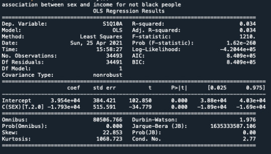
I want to measure the association between the variable SEX and income, and check if being a Black people or not (my moderator) will make the association stronger or different. 

First, I analyzed the association between income and sex and verified that there is a significant association. 

the p-value is significant. 

then I create a data frame with income, sex, and being Black; and data frame with income, sex, and being not Black

 I run the Anova with the two different groups finding the p-value significant for both. 

After that I printed the mean for both the groups.

Based on the study, being Black increases the income but not as being not black. 

here is the bar graph that summarize the results

Bivariate bar graph for Black people

Bivariate bar graph for NOT Black people

Here all the script

import numpy import pandas import statsmodels.formula.api as smf import statsmodels.stats.multicomp as multi

data = pandas.read_csv('nesarc.csv', low_memory=False)

data['S1Q10A'] = pandas.to_numeric(data['S1Q10A'])

sub1 = data[['SEX', 'S1Q10A']].dropna()

model2 = smf.ols(formula='S1Q10A ~ C(SEX)', data=sub1).fit() print (model2.summary())

print ('means for INCOME by SEX') m1= sub1.groupby('SEX').mean() print (m1)

print ('standard deviations for INCOME by SEX') sd1 = sub1.groupby('SEX').std() print (sd1)

import seaborn import matplotlib.pyplot as plt

#bivariate bar graph seaborn.catplot (x='SEX', y='S1Q10A', data=sub1, kind='bar', ci=None) plt.xlabel('sex') plt.ylabel('income')

sub2 = data[['SEX', 'S1Q10A','S1Q1D3']].dropna() print(sub2)

test1 = sub2.where(sub2['S1Q1D3'] == 1).dropna() print(test1)

test2 = sub2.where(sub2['S1Q1D3'] == 2).dropna() print(test2)

print ('association between sex and income for black people') model2 = smf.ols(formula='S1Q10A ~ C(SEX)', data=test1).fit() print (model2.summary())

print ('association between sex and income for not black people') model2 = smf.ols(formula='S1Q10A ~ C(SEX)', data=test2).fit() print (model2.summary())

print ("means for Income by SEX  for Black people") m3= test1.groupby('SEX').mean() print(m3)

print ("means for Income by SEX  for not Black people") m3= test2.groupby('SEX').mean() print(m3)

#bivariate bar graph for Black people seaborn.catplot (x='SEX', y='S1Q10A', data=test1, kind='bar', ci=None) plt.xlabel('sex') plt.ylabel('income')

#bivariate bar graph for not Black people seaborn.catplot (x='SEX', y='S1Q10A', data=test2, kind='bar', ci=None) plt.xlabel('sex') plt.ylabel('income')

[lucacode]

WEEK 3

I decided to examine the relation between 2 quantitative variables:

Income per year

number of persone in house

I asked python to do a scatterplot with the following code:

scat1 = seaborn.regplot(x="NUMPERS", y="S1Q10A", fit_reg=True, data=data) plt.xlabel('Number person in house') plt.ylabel('Income per year') plt.title('Scatterplot for the Association Between persone in house and income per year')

From the scatterplot we can see a negative linear relationship. 

I run the Pearson correlation with the following code:

data_clean=data.dropna()

print ('Association Between persone in house and income per year') print (scipy.stats.pearsonr(data_clean['NUMPERS'], data_clean['S1Q10A']))

Even though my p-value is very significant, the association is negative, but very weak. -0.036 (r)

the r2 is: 0.00129, which means that I can predict the 0.129% of the variability we'll see in the rate of Income per year.

[lucacode]

week2

I decided to see the association between the variable tabacco dependence and use of cannabis in a year. 

- First of all I need to create a new variable with the frequency of smoking cannabis during an year. I use this code.

# recode missing values to python missing (NaN) data['S3BD5Q2C']=data['S3BD5Q2C'].replace(99, numpy.nan)

#recoding values for S3BD5Q2C into a new variable, USFREQY recode1 = {1: 365, 2: 312, 3: 208 , 4: 104, 5: 36, 6: 12, 7: 11, 8: 6, 9: 2, 10: 1} data['USFREQY']= data['S3BD5Q2C'].map(recode1)

- second: I looked at the contingency table of observed counts,  column percentages and chi-square to see if there in any association between the variables. 

# contingency table of observed counts ct1=pandas.crosstab(data['TAB12MDX'], data['USFREQY']) print (ct1)

# column percentages colsum=ct1.sum(axis=0) colpct=ct1/colsum print(colpct)

# chi-square print ('chi-square value, p value, expected counts') cs1= scipy.stats.chi2_contingency(ct1) print (cs1)

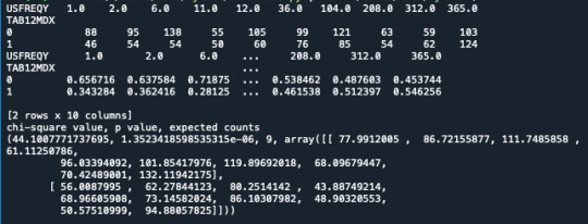
The p value is 1.35e-06 which means the p value is very low. Therefore, there is a valid statistic association between the two variables tabacco dependence and use of cannabis in a year. 

I also decided to do a graph of my variables.

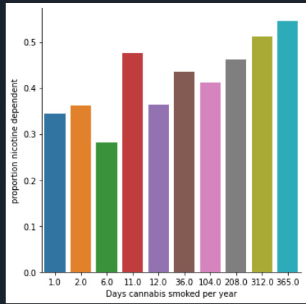
I can say that I can accept the alternate hypothesis that not all nicotine dependence rates are equal across smoking cannabis per year category. 

Now, I have to run a post-hoc to understand which of the category are equal and which are not.

I have 45 combination between my category, therefore my p-value is 0.05/45 = 0.00111111. 

This in an example of code that I used for each category:

# chi-square for set 1/45 recode2 = {1: 1, 2: 2} data['COMP1v2']= data['USFREQY'].map(recode2)

# contingency table of observed counts ct2=pandas.crosstab(data['TAB12MDX'], data['COMP1v2']) print (ct2)

# column percentages colsum=ct2.sum(axis=0) colpct=ct2/colsum print(colpct)

print ('chi-square value, p value, expected counts') cs2= scipy.stats.chi2_contingency(ct2) print (cs2)

I filled a table with the p-value

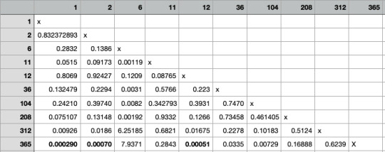
I have found that the groups 1-365; 2-265; 12-365 have a significant difference.

To summarize:

There is a significant association between groups 1-365; 2-265; 12-365

[lucacode]

Week 1

I decided to examine the variance between a Categorical variable (the presence of the father in house - FATHERIH) with a quantitative variable (how many person live in the house - NUMREL). 

First I set my data:

import numpy import pandas import statsmodels.formula.api as smf import statsmodels.stats.multicomp as multi

data = pandas.read_csv('nesarc.csv', low_memory=False)

data['FATHERIH'] = pandas.to_numeric(data['FATHERIH']) data['NUMREL'] = pandas.to_numeric(data['NUMREL'])

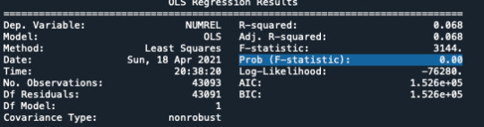
Second I used the ANOVA to see if my is significant. 

# using ols function for calculating the F-statistic and associated p value model1 = smf.ols(formula='NUMREL ~ C(FATHERIH)', data=data) results1 = model1.fit() print (results1.summary())

With surprise, I have a significant p=0.00, which means I can reject my null Hypothesis (no association between the 2 variables). 

Third: I asked python to tell the mean and s.d. of the variable NUMREL (number of relatives in house) to see if there is a difference between the mean of NUMREL with father in house or without. 

sub2 = data[['NUMREL', 'FATHERIH']].dropna()

print ('means for FATHERIH by NUMBER OF RELATIVES AT HOME') m1= sub2.groupby('FATHERIH').mean() print (m1)

print ('standard deviations for FATHERIH by NUMBER OF RELATIVES AT HOME') sd1 = sub2.groupby('FATHERIH').std() print (sd1)

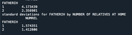
I can conclude that the mean is significant, and there is an association between the two variables. 

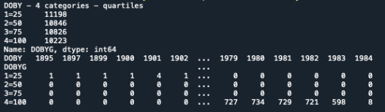
To do more exercises and use the POST HOC analysis, I used an other quantitative variable that I grouped in 4 groups (date of birth by Year, and I divided it in 4 percentiles group).

In the Console it shows that the variable has been divided in 4 groups. The new variable is named DOBYG. But when I try to use it, it doesn’t work because python seems to use still the variable not grouped. 

I tried different options but it doesn’t work. 

I run the POST HOC test too, but something is wrong. here the code:

#SPLIT VARIABLE NUMREL IN 4 GROUPS, percentile print('DOBY - 4 categories - quartiles') data['DOBYG']=pandas.qcut(data.DOBY, 4, labels=["1=25", "2=50", "3=75", "4=100"]) c1 = data['DOBYG'].value_counts(sort=False, dropna=True) print(c1)

print(pandas.crosstab(data['DOBYG'],data['DOBY']))

data['DOBYG'] = pandas.to_numeric(data['DOBY'])

sub1 = data[['DOBYG', 'NUMREL']].dropna()

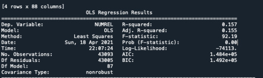
model2 = smf.ols(formula='NUMREL ~ C(DOBYG)', data=sub1).fit() print (model2.summary())

print ('means for NUMREL by DOBYG') m1= sub1.groupby('DOBYG').mean() print (m1)

print ('standard deviations for NUMREL by DOBYG') sd1 = sub1.groupby('DOBYG').std() print (sd1)

Then I ask the mean ask s.d. for the variable DOBYG. 

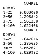
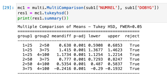
I run the POST HOC test, and every my category is True

[lucacode]

Week 4

Step 1: I take a categorical variable H1G14, and a quantitative variable (USFREQMO), and made two different graphs. Here is the code I used:

import pandas import numpy import seaborn import matplotlib.pyplot as plt

# change format from numeric to categorial

data['H1GI4'] =data['H1GI4'].astype('category') data['H1HS1'] =data['H1HS1'].astype('category') data['H1DA3'] =data['H1DA3'].astype('category')

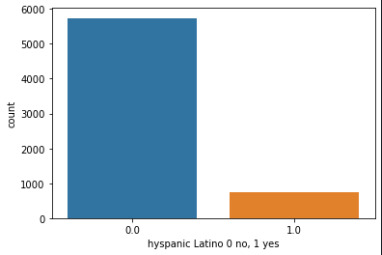
seaborn.countplot(x='H1GI4', data=sub2) plt.xlabel('hyspanic Latino 0 no, 1 yes')

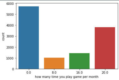
seaborn.countplot(x='USFREQMO', data=data) plt.xlabel('how many time you play game per month')

Also, I examined the measures of center and spread for the variable USFREQMO, using the following code:

print('describe number of time played oer month') desc1 = data['USFREQMO'].describe() print(desc1)

STep 2: 

I decided to analyze the relation between two variables. Both categorical, but one has more than 2 categories. 

First, I created just two categories for that variable:

# creating categorical variable for H1GH1 with 2 categories

def HEALTH (row):    if row['H1GH1'] < 3 :        return 1    if row['H1GH1'] > 3 :        return 0

After that I compared them:

  # bivariate bar graph 

seaborn.catplot(x='USFREQMO', y='H1GH1', data=data, kind='bar', ci=None) plt.xlabel('play per Month') plt.ylabel('General health')

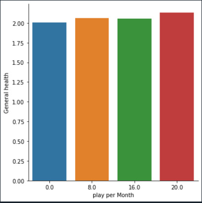
Form the graph it seems there is not an important relation between the number of times a individual plays games or watches tv during the month, and their health situation 

[lucacode]

Week 3

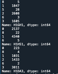
I started counting the values of 3 variables:

print('counts for original')

c1A = data['H1GH1'].value_counts(sort=False) c1B = data['H1HS1'].value_counts(sort=False) c1C = data['H1DA3'].value_counts(sort=False) print(c1A) print(c1B) print(c1B)

Here is the outcome:

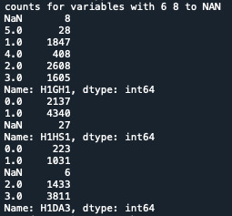
After that, I identified my mission data: for each Variable, the number 6 and 8 are missing data. I changes these values in NaN using this code:

data['H1DA3']=data['H1DA3'].replace(6,numpy.nan) data['H1DA3']=data['H1DA3'].replace(8,numpy.nan)

data['H1GH1']=data['H1GH1'].replace(6,numpy.nan) data['H1GH1']=data['H1GH1'].replace(8,numpy.nan)

data['H1HS1']=data['H1HS1'].replace(6,numpy.nan) data['H1HS1']=data['H1HS1'].replace(8,numpy.nan)

print('counts for variables with 6 8 to NAN') c2A = data['H1GH1'].value_counts(sort=False, dropna=False) c2B = data['H1HS1'].value_counts(sort=False, dropna=False) c2C = data['H1DA3'].value_counts(sort=False, dropna=False) print(c2A) print(c2B) print(c2C)

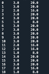
Third step, I recoded the variable H1DA3 using different numbers. Therefore I set the value 1,2,3 as number of time that a person watch tv/play games in a month. Since my data are a bit different from the video, I did have to multiply and create a second variable. I just needed to create a secondary variable using the recode:

print('recode H1DA3 per month') recode1 = {1: 8, 2:16, 3:20} data['USFREQMO']= data['H1DA3'].map(recode1)

c3C = data['USFREQMO'].value_counts(sort=False, dropna=False) print(c3C)

print('table with counting') sub1=data[['H1DA3', 'USFREQMO']] a = sub1.head(n=25) print(a)

STEP 4:

I wrote the code that they suggested for my data set. Using the Ethnicity variable:

print('converting in numeric data') data['H1GI4'] = pandas.to_numeric(data['H1GI4']) data['H1GI6A'] = pandas.to_numeric(data['H1GI6A']) data['H1GI6B'] = pandas.to_numeric(data['H1GI6B']) data['H1GI6C'] = pandas.to_numeric(data['H1GI6C']) data['H1GI6D'] = pandas.to_numeric(data['H1GI6D'])

print('replacing missing data') data['H1GI4'] = data['H1GI4'].replace([6, 8], numpy.nan) data['H1GI6A'] = data['H1GI6A'].replace([6, 8], numpy.nan) data['H1GI6B'] = data['H1GI6B'].replace([6, 8], numpy.nan) data['H1GI6C'] = data['H1GI6C'].replace([6, 8], numpy.nan) data['H1GI6D'] = data['H1GI6D'].replace([6, 8], numpy.nan)

print('summing data in a new variable') data['NUMETHNIC'] = data['H1GI4'] + data['H1GI6A'] + data['H1GI6B'] + data['H1GI6C'] + data['H1GI6D']

print('counts for NUMETHNIC value') chk8 = data["NUMETHNIC"].value_counts(sort=False, dropna=False) print(chk8)

def ETHNICITY (row):    if row['NUMETHNIC'] > 1:        return 1    if row['H1GI4'] == 1:        return 2    if row['H1GI6A'] == 1:         return 3    if row['H1GI6B'] == 1:         return 4    if row['H1GI6C'] == 1:         return 5    if row['H1GI6D'] == 1:         return 6

data['ETHNICITY']  = data.apply (lambda row: ETHNICITY (row), axis=1)

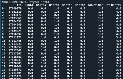
sub2 = data[['AID', 'H1GI4', 'H1GI6A', 'H1GI6B', 'H1GI6C', 'H1GI6D', 'NUMETHNIC', 'ETHNICITY']] a = sub2.head(n=25) print(a)

c10 = sub2['H1GI4'].value_counts(sort=False) print(c10)

[lucacode]

Week 2

import pandas import numpy

data = pandas.read_csv('addhealth_pds.csv', low_memory=False)

print(len(data)) print(len(data.columns))

data['H1HS1'] = pandas.to_numeric(data['H1HS1']) data['H1HS1'].dtype data['H1GH1'] = pandas.to_numeric(data['H1GH1'])

print('counts for H1HS1') c1 = data['H1HS1'].value_counts(sort=False) print(c1)

print('percentage for H1HS1') p1 = data['H1HS1'].value_counts(sort=False, normalize=True)   print(p1)

print('counts for H1GH1') c2 = data['H1GH1'].value_counts(sort=False) print(c2)

print('percentage for H1GH1') p2 = data['H1GH1'].value_counts(sort=False, normalize=True) print(p2)

print('counts for H1DA3') c3 = data['H1DA3'].value_counts(sort=False) print(c3)

print('percentage for H1DA3') p3 = data['H1DA3'].value_counts(sort=False, normalize=True) print(p3)

sub1 = data[(data['H1DA3'] == 3) & (data['H1GH1'] == 6) & (data['H1GH1'] == 1)]

sub2=sub1.copy()

print('counts for H1GH1') c4 = sub1['H1GH1'].value_counts(sort=False) print(c2)

print('percentage for H1GH1') p2 = sub2['H1GH1'].value_counts(sort=False, normalize=True)   print(p2)

print('counts for H1DA3') c3 = sub2['H1DA3'].value_counts(sort=False) print(c3)

print('percentage for H1DA3') p3 = sub2['H1DA3'].value_counts(sort=False, normalize=True)   print(p3)

here my output:

ounts for H1HS1 0    2137 8      22 1    4340 6       5 Name: H1HS1, dtype: int64 percentage for H1HS1 0    0.328567 8    0.003383 1    0.667282 6    0.000769 Name: H1HS1, dtype: float64

counts for H1GH1 4     408 8       5 1    1847 5      28 2    2608 6       3 3    1605 Name: H1GH1, dtype: int64 percentage for H1GH1 4    0.062731 8    0.000769 1    0.283979 5    0.004305 2    0.400984 6    0.000461 3    0.246771 Name: H1GH1, dtype: float64

I am interested in looking at H1GH1 (which is your health situation) that respond 1-excellent, and 6-poor).

0,28% responded 1

0.26% responded 6

counts for H1DA3 0     223 8       4 1    1031 2    1433 6       2 3    3811 Name: H1DA3, dtype: int64 percentage for H1DA3 0    0.034287 8    0.000615 1    0.158518 2    0.220326 6    0.000308 3    0.585947 Name: H1DA3, dtype: float64

I am interested in looking at H1DA3 (which is how many times during the week you watch th) that respond 3: 5 times a week

3    0.585947%

It seems I didn’t have any missing data. 

Also, I tried to do a table for frequency but I didn’t find any explanation for that in the videos!

[lucacode]

[lucacode]

Week 2

I really don’t know what I am doing wrong. 

I'm trying to work on add health and seeing the frequency of 3 variables (H1HS1 - H1GH1 - H1DA3) but when I run the the commands nothing happens. 

very frustrating. I don’t know what to do

[lucacode]

Peer-graded Assignment: Getting Your Research Project Started

Step 1: I decided to use the National Longitudinal Study of Adolescent Health (AddHealth). I am interested in the friendship that adolescence have, and pair of sibling. I am interested to check if there is any association between the pair of sibling (Male/male, Female/male, etc) and the friendship that they have (in school/in home friendship). 

Bibliography

In this paper the authors discuss the association between friendship and sibling relationship, demonstrating that the two elements are connected.

Kramer, L., & Kowal, A. K. (2005). Sibling relationship quality from birth to adolescence: the enduring contributions of friends. Journal of Family Psychology, 19(4), 503–511. https://doi.org/10.1037/0893-3200.19.4.503

In another article the authors found that “For girls, a good relationship with their siblings was linked to good relationships with their parents and peers, as well as increased self-esteem and life satisfaction. For boys, sibling relationships had no relation with other family or personal variables.”

- Alfredo Oliva & Enrique Arranz (2005) Sibling relationships during adolescence, European Journal of Developmental Psychology, 2:3, 253-270, DOI: 10.1080/17405620544000002

Is the variable “full sibling -FSFFxxx - GSMMxxx” related with the variable MF_AID1?

My hypothesis is that sibling with different gender are more likely to look for friends outside school, because they are more flexible about meeting different peers.

[lucacode]

Welcome

trial