machine-learning-coursera

[machine-learning-coursera]

Machine Learning for Data Analysis

Week 4: Running a k-means Cluster Analysis

A k-means cluster analysis was conducted to identify underlying subgroups of countries based on their similarity of responses on 7 variables that represent characteristics that could have an impact on internet use rates. Clustering variables included quantitative variables measuring income per person, employment rate, female employment rate, polity score, alcohol consumption, life expectancy, and urban rate. All clustering variables were standardized to have a mean of 0 and a standard deviation of 1.

Because the GapMinder dataset which I am using is relatively small (N < 250), I have not split the data into test and training sets. A series of k-means cluster analyses were conducted on the training data specifying k=1-9 clusters, using Euclidean distance. The variance in the clustering variables that was accounted for by the clusters (r-square) was plotted for each of the nine cluster solutions in an elbow curve to provide guidance for choosing the number of clusters to interpret.

Load the data, set the variables to numeric, and clean the data of NA values

In [1]:import pandas as pd import numpy as np import matplotlib.pyplot as plt import statsmodels.formula.api as smf import statsmodels.stats.multicomp as multi from sklearn.cross_validation import train_test_split from sklearn import preprocessing from sklearn.cluster import KMeans data = pd.read_csv('c:/users/greg/desktop/gapminder.csv', low_memory=False) data['internetuserate'] = pd.to_numeric(data['internetuserate'], errors='coerce') data['incomeperperson'] = pd.to_numeric(data['incomeperperson'], errors='coerce') data['employrate'] = pd.to_numeric(data['employrate'], errors='coerce') data['femaleemployrate'] = pd.to_numeric(data['femaleemployrate'], errors='coerce') data['polityscore'] = pd.to_numeric(data['polityscore'], errors='coerce') data['alcconsumption'] = pd.to_numeric(data['alcconsumption'], errors='coerce') data['lifeexpectancy'] = pd.to_numeric(data['lifeexpectancy'], errors='coerce') data['urbanrate'] = pd.to_numeric(data['urbanrate'], errors='coerce') sub1 = data.copy() data_clean = sub1.dropna()

Subset the clustering variables

In [2]:cluster = data_clean[['incomeperperson','employrate','femaleemployrate','polityscore', 'alcconsumption', 'lifeexpectancy', 'urbanrate']] cluster.describe()

Out[2]:incomeperpersonemployratefemaleemployratepolityscorealcconsumptionlifeexpectancyurbanratecount150.000000150.000000150.000000150.000000150.000000150.000000150.000000mean6790.69585859.26133348.1006673.8933336.82173368.98198755.073200std9861.86832710.38046514.7809996.2489165.1219119.90879622.558074min103.77585734.90000212.400000-10.0000000.05000048.13200010.40000025%592.26959252.19999939.599998-1.7500002.56250062.46750036.41500050%2231.33485558.90000248.5499997.0000006.00000072.55850057.23000075%7222.63772165.00000055.7250009.00000010.05750076.06975071.565000max39972.35276883.19999783.30000310.00000023.01000083.394000100.000000

Standardize the clustering variables to have mean = 0 and standard deviation = 1

In [3]:clustervar=cluster.copy() clustervar['incomeperperson']=preprocessing.scale(clustervar['incomeperperson'].astype('float64')) clustervar['employrate']=preprocessing.scale(clustervar['employrate'].astype('float64')) clustervar['femaleemployrate']=preprocessing.scale(clustervar['femaleemployrate'].astype('float64')) clustervar['polityscore']=preprocessing.scale(clustervar['polityscore'].astype('float64')) clustervar['alcconsumption']=preprocessing.scale(clustervar['alcconsumption'].astype('float64')) clustervar['lifeexpectancy']=preprocessing.scale(clustervar['lifeexpectancy'].astype('float64')) clustervar['urbanrate']=preprocessing.scale(clustervar['urbanrate'].astype('float64'))

Split the data into train and test sets

In [4]:clus_train, clus_test = train_test_split(clustervar, test_size=.3, random_state=123)

Perform k-means cluster analysis for 1-9 clusters

In [5]:from scipy.spatial.distance import cdist clusters = range(1,10) meandist = [] for k in clusters: model = KMeans(n_clusters = k) model.fit(clus_train) clusassign = model.predict(clus_train) meandist.append(sum(np.min(cdist(clus_train, model.cluster_centers_, 'euclidean'), axis=1)) / clus_train.shape[0])

Plot average distance from observations from the cluster centroid to use the Elbow Method to identify number of clusters to choose

In [6]:plt.plot(clusters, meandist) plt.xlabel('Number of clusters') plt.ylabel('Average distance') plt.title('Selecting k with the Elbow Method') plt.show()

Interpret 3 cluster solution

In [7]:model3 = KMeans(n_clusters=4) model3.fit(clus_train) clusassign = model3.predict(clus_train)

Plot the clusters

In [8]:from sklearn.decomposition import PCA pca_2 = PCA(2) plt.figure() plot_columns = pca_2.fit_transform(clus_train) plt.scatter(x=plot_columns[:,0], y=plot_columns[:,1], c=model3.labels_,) plt.xlabel('Canonical variable 1') plt.ylabel('Canonical variable 2') plt.title('Scatterplot of Canonical Variables for 4 Clusters') plt.show()

Begin multiple steps to merge cluster assignment with clustering variables to examine cluster variable means by cluster.

Create a unique identifier variable from the index for the cluster training data to merge with the cluster assignment variable.

In [9]:clus_train.reset_index(level=0, inplace=True)

Create a list that has the new index variable

In [10]:cluslist = list(clus_train['index'])

Create a list of cluster assignments

In [11]:labels = list(model3.labels_)

Combine index variable list with cluster assignment list into a dictionary

In [12]:newlist = dict(zip(cluslist, labels)) print (newlist) {2: 1, 4: 2, 6: 0, 10: 0, 11: 3, 14: 2, 16: 3, 17: 0, 19: 2, 22: 2, 24: 3, 27: 3, 28: 2, 29: 2, 31: 2, 32: 0, 35: 2, 37: 3, 38: 2, 39: 3, 42: 2, 45: 2, 47: 1, 53: 3, 54: 3, 55: 1, 56: 3, 58: 2, 59: 3, 63: 0, 64: 0, 66: 3, 67: 2, 68: 3, 69: 0, 70: 2, 72: 3, 77: 3, 78: 2, 79: 2, 80: 3, 84: 3, 88: 1, 89: 1, 90: 0, 91: 0, 92: 0, 93: 3, 94: 0, 95: 1, 97: 2, 100: 0, 102: 2, 103: 2, 104: 3, 105: 1, 106: 2, 107: 2, 108: 1, 113: 3, 114: 2, 115: 2, 116: 3, 123: 3, 126: 3, 128: 3, 131: 2, 133: 3, 135: 2, 136: 0, 139: 0, 140: 3, 141: 2, 142: 3, 144: 0, 145: 1, 148: 3, 149: 2, 150: 3, 151: 3, 152: 3, 153: 3, 154: 3, 158: 3, 159: 3, 160: 2, 173: 0, 175: 3, 178: 3, 179: 0, 180: 3, 183: 2, 184: 0, 186: 1, 188: 2, 194: 3, 196: 1, 197: 2, 200: 3, 201: 1, 205: 2, 208: 2, 210: 1, 211: 2, 212: 2}

Convert newlist dictionary to a dataframe

In [13]:newclus = pd.DataFrame.from_dict(newlist, orient='index') newclus

Out[13]:0214260100113142163170192222243273282292312320352373382393422452471533543551563582593630......145114831492150315131523153315431583159316021730175317831790180318321840186118821943196119722003201120522082210121122122

105 rows × 1 columns

Rename the cluster assignment column

In [14]:newclus.columns = ['cluster']

Repeat previous steps for the cluster assignment variable

Create a unique identifier variable from the index for the cluster assignment dataframe to merge with cluster training data

In [15]:newclus.reset_index(level=0, inplace=True)

Merge the cluster assignment dataframe with the cluster training variable dataframe by the index variable

In [16]:merged_train = pd.merge(clus_train, newclus, on='index') merged_train.head(n=100)

Out[16]:indexincomeperpersonemployratefemaleemployratepolityscorealcconsumptionlifeexpectancyurbanratecluster0159-0.393486-0.0445910.3868770.0171271.843020-0.0160990.79024131196-0.146720-1.591112-1.7785290.498818-0.7447360.5059900.6052111270-0.6543650.5643511.0860520.659382-0.727105-0.481382-0.2247592329-0.6791572.3138522.3893690.3382550.554040-1.880471-1.9869992453-0.278924-0.634202-0.5159410.659382-0.1061220.4469570.62033335153-0.021869-1.020832-0.4073320.9805101.4904110.7233920.2778493635-0.6665191.1636281.004595-0.785693-0.715352-2.084304-0.7335932714-0.6341100.8543230.3733010.177691-1.303033-0.003846-1.24242828116-0.1633940.119726-0.3394510.338255-1.1659070.5304950.67993439126-0.630263-1.446126-0.3055100.6593823.1711790.033923-0.592152310123-0.163655-0.460219-0.8010420.980510-0.6448300.444628-0.560127311106-0.640452-0.2862350.1153530.659382-0.247166-2.104758-1.317152212142-0.635480-0.808186-0.7874660.0171271.155433-1.731823-0.29859331389-0.615980-2.113062-2.423400-0.625129-1.2442650.0060770.512695114160-0.6564731.9852172.199302-1.1068200.620643-1.371039-1.63383921556-0.430694-0.102586-0.2240530.659382-0.5547190.3254460.250272316180-0.559059-0.402224-0.6041870.338255-1.1776610.603401-1.777949317133-0.419521-1.668438-0.7331610.3382551.032020-0.659900-0.81098631831-0.618282-0.0155940.061048-1.2673840.211226-1.7590620.075026219171.801349-1.030498-0.4344840.6593820.7029191.1165791.8808550201450.447771-0.827517-1.731013-1.909640-1.1561120.4042250.7359771211000.974856-0.034925-0.0068330.6593822.4150301.1806761.173646022178-0.309804-1.755430-0.9368040.8199460.653945-1.6388680.2520513231732.6193200.3033760.217174-0.946256-1.0346581.2296851.99827802459-0.056177-0.2669040.2714790.8199462.0408730.5916550.63990432568-0.562821-0.3538960.0271070.338255-0.0316830.481486-0.1037773261080.111383-1.030498-1.690284-1.749076-1.3167450.5879080.999290127212-0.6582520.7286690.678765-0.464565-0.364702-1.781946-0.78874722819-0.6525281.1926250.6855540.498818-0.928876-1.306335-0.617060229188-0.662484-0.4505530.135717-1.106820-0.672255-0.147127-1.2726732..............................70140-0.594402-0.044591-0.8214060.819946-0.3157280.5125720.074137371148-0.0905570.052066-0.3190860.8199460.0936890.7235950.80625437211-0.4523170.1583900.549792-1.7490761.2768870.177913-0.140250373641.636776-0.779188-0.1697480.8199461.1084191.2715050.99128407484-0.117682-1.156153-0.5295180.9805101.8214720.5500380.5527263751750.604211-0.3248980.0882000.9805101.5903171.048938-0.287918376197-0.481087-0.0735890.393665-2.070203-0.356866-0.404628-0.287029277183-0.506714-0.808186-0.067926-2.070203-0.347071-2.051902-1.340281278210-0.628790-1.958410-1.887139-0.946256-1.297156-0.353290-1.08675317954-0.5150780.042400-0.1765360.1776910.5109430.6733710.467327380114-0.6661982.2945212.111056-0.625129-1.077755-0.229248-1.1365692814-0.5503841.5889211.445822-0.946256-0.245207-1.8114130.072358282911.575455-0.769523-0.1154430.980510-0.8426821.2795041.62732708377-0.5015740.332373-0.2783580.6593820.0545110.221758-0.28880838466-0.265535-0.0252600.305419-0.1434370.516820-0.6358011.332879385921.240375-1.243145-0.8349830.9805100.5677521.3035020.5785230862011.4545511.540592-0.733161-1.909640-1.2344700.7659211.014413187105-0.004485-1.281808-1.7513770.498818-0.8857790.3704051.418278188205-0.593947-0.1702460.305419-2.070203-0.629158-0.070373-0.8118762891540.504036-0.1605810.1696570.9805101.3846291.0649370.19511839045-0.6307520.061732-0.678856-0.625129-0.068902-1.377621-0.27991229197-0.6432031.3472771.2557550.498818-0.576267-1.199710-1.488839292632.067368-0.1992430.3597250.9805101.2298731.1133390.365916093211-0.6469130.1680550.3665130.498818-0.638953-2.020815-0.874146294158-0.422620-0.943506-0.2919340.8199461.8273490.505990-0.037060395135-0.6635950.2453810.4411820.338255-0.862272-0.018934-1.68276529679-0.6744750.6416770.1221410.338255-0.572349-2.111239-1.1223362971790.882197-0.653534-0.4344840.9805100.9810881.2578350.980609098149-0.6151691.0766361.4118810.017127-0.623282-0.626890-1.891814299113-0.464904-2.354706-1.4459120.8199460.4149550.5938830.5260393

100 rows × 9 columns

Cluster frequencies

In [17]:merged_train.cluster.value_counts()

Out[17]:3 39 2 35 0 18 1 13 Name: cluster, dtype: int64

Calculate clustering variable means by cluster

In [18]:clustergrp = merged_train.groupby('cluster').mean() print ("Clustering variable means by cluster") clustergrp Clustering variable means by cluster

Out[18]:indexincomeperpersonemployratefemaleemployratepolityscorealcconsumptionlifeexpectancyurbanratecluster093.5000001.846611-0.1960210.1010220.8110260.6785411.1956961.0784621117.461538-0.154556-1.117490-1.645378-1.069767-1.0827280.4395570.5086582100.657143-0.6282270.8551520.873487-0.583841-0.506473-1.034933-0.8963853107.512821-0.284648-0.424778-0.2000330.5317550.6146160.2302010.164805

Validate clusters in training data by examining cluster differences in internetuserate using ANOVA. First, merge internetuserate with clustering variables and cluster assignment data

In [19]:internetuserate_data = data_clean['internetuserate']

Split internetuserate data into train and test sets

In [20]:internetuserate_train, internetuserate_test = train_test_split(internetuserate_data, test_size=.3, random_state=123) internetuserate_train1=pd.DataFrame(internetuserate_train) internetuserate_train1.reset_index(level=0, inplace=True) merged_train_all=pd.merge(internetuserate_train1, merged_train, on='index') sub5 = merged_train_all[['internetuserate', 'cluster']].dropna()

In [21]:internetuserate_mod = smf.ols(formula='internetuserate ~ C(cluster)', data=sub5).fit() internetuserate_mod.summary()

Out[21]:

OLS Regression ResultsDep. Variable:internetuserateR-squared:0.679Model:OLSAdj. R-squared:0.669Method:Least SquaresF-statistic:71.17Date:Thu, 12 Jan 2017Prob (F-statistic):8.18e-25Time:20:59:17Log-Likelihood:-436.84No. Observations:105AIC:881.7Df Residuals:101BIC:892.3Df Model:3Covariance Type:nonrobustcoefstd errtP>|t|[95.0% Conf. Int.]Intercept75.20683.72720.1770.00067.813 82.601C(cluster)[T.1]-46.95175.756-8.1570.000-58.370 -35.534C(cluster)[T.2]-66.56684.587-14.5130.000-75.666 -57.468C(cluster)[T.3]-39.48604.506-8.7630.000-48.425 -30.547Omnibus:5.290Durbin-Watson:1.727Prob(Omnibus):0.071Jarque-Bera (JB):4.908Skew:0.387Prob(JB):0.0859Kurtosis:3.722Cond. No.5.90

Means for internetuserate by cluster

In [22]:m1= sub5.groupby('cluster').mean() m1

Out[22]:internetuseratecluster075.206753128.25501828.639961335.720760

Standard deviations for internetuserate by cluster

In [23]:m2= sub5.groupby('cluster').std() m2

Out[23]:internetuseratecluster014.093018121.75775228.399554319.057835

In [24]:mc1 = multi.MultiComparison(sub5['internetuserate'], sub5['cluster']) res1 = mc1.tukeyhsd() res1.summary()

Out[24]:

Multiple Comparison of Means - Tukey HSD,FWER=0.05group1group2meandifflowerupperreject01-46.9517-61.9887-31.9148True02-66.5668-78.5495-54.5841True03-39.486-51.2581-27.7139True12-19.6151-33.0335-6.1966True137.4657-5.76520.6965False2327.080817.461736.6999True

The elbow curve was inconclusive, suggesting that the 2, 4, 6, and 8-cluster solutions might be interpreted. The results above are for an interpretation of the 4-cluster solution.

In order to externally validate the clusters, an Analysis of Variance (ANOVA) was conducting to test for significant differences between the clusters on internet use rate. A tukey test was used for post hoc comparisons between the clusters. Results indicated significant differences between the clusters on internet use rate (F=71.17, p<.0001). The tukey post hoc comparisons showed significant differences between clusters on internet use rate, with the exception that clusters 0 and 2 were not significantly different from each other. Countries in cluster 1 had the highest internet use rate (mean=75.2, sd=14.1), and cluster 3 had the lowest internet use rate (mean=8.64, sd=8.40).

[machine-learning-coursera]

Machine Learning for Data Analysis

Week 3: Running a Lasso Regression Analysis

Continuing on the machine learning analysis of internet use rate from the GapMinder dataset, I conducted a lasso regression analysis to identify a subset of variables from a pool of 10 quantitative predictor variables that best predicted a quantitative response variable measuring the internet use rates of the countries in the world. I have added several variables to my standard analysis that are not particularly interesting to my main question of how internet use rates of a country affects income in order to have more variables available for this lasso regression. The explanatory variables I have used in this model are income per person, employment rate, female employment rate, polity score, alcohol consumption, life expectancy, oil per person, electricity use per person, and urban rate. All variables have been normalized to have a mean of zero and standard deviation of one.

Load the data, convert all variables to numeric, and discard NA values

In [1]:'import pandas as pd import numpy as np import matplotlib.pyplot as plt from sklearn.cross_validation import train_test_split from sklearn.linear_model import LassoLarsCV data = pd.read_csv('c:/users/greg/desktop/gapminder.csv', low_memory=False) data['internetuserate'] = pd.to_numeric(data['internetuserate'], errors='coerce') data['incomeperperson'] = pd.to_numeric(data['incomeperperson'], errors='coerce') data['employrate'] = pd.to_numeric(data['employrate'], errors='coerce') data['femaleemployrate'] = pd.to_numeric(data['femaleemployrate'], errors='coerce') data['polityscore'] = pd.to_numeric(data['polityscore'], errors='coerce') data['alcconsumption'] = pd.to_numeric(data['alcconsumption'], errors='coerce') data['lifeexpectancy'] = pd.to_numeric(data['lifeexpectancy'], errors='coerce') data['oilperperson'] = pd.to_numeric(data['oilperperson'], errors='coerce') data['relectricperperson'] = pd.to_numeric(data['relectricperperson'], errors='coerce') data['urbanrate'] = pd.to_numeric(data['urbanrate'], errors='coerce') sub1 = data.copy() data_clean = sub1.dropna()

Select predictor variables and target variable as separate data sets

In [3]:predvar = data_clean[['incomeperperson','employrate','femaleemployrate','polityscore', 'alcconsumption', 'lifeexpectancy', 'oilperperson', 'relectricperperson', 'urbanrate']] target = data_clean.internetuserate

Standardize predictors to have mean = 0 and standard deviation = 1

In [4]:predictors=predvar.copy() from sklearn import preprocessing predictors['incomeperperson']=preprocessing.scale(predictors['incomeperperson'].astype('float64')) predictors['employrate']=preprocessing.scale(predictors['employrate'].astype('float64')) predictors['femaleemployrate']=preprocessing.scale(predictors['femaleemployrate'].astype('float64')) predictors['polityscore']=preprocessing.scale(predictors['polityscore'].astype('float64')) predictors['alcconsumption']=preprocessing.scale(predictors['alcconsumption'].astype('float64')) predictors['lifeexpectancy']=preprocessing.scale(predictors['lifeexpectancy'].astype('float64')) predictors['oilperperson']=preprocessing.scale(predictors['oilperperson'].astype('float64')) predictors['relectricperperson']=preprocessing.scale(predictors['relectricperperson'].astype('float64')) predictors['urbanrate']=preprocessing.scale(predictors['urbanrate'].astype('float64'))

Split data into train and test sets

In [6]:pred_train, pred_test, tar_train, tar_test = train_test_split(predictors, target, test_size=.3, random_state=123)

Specify the lasso regression model

In [7]:model=LassoLarsCV(cv=10, precompute=False).fit(pred_train,tar_train)

Print the regression coefficients

In [9]:dict(zip(predictors.columns, model.coef_))

Out[9]:{'alcconsumption': 6.2210718136158443, 'employrate': 0.0, 'femaleemployrate': 0.0, 'incomeperperson': 10.730391071065633, 'lifeexpectancy': 7.9415161171462634, 'oilperperson': 0.0, 'polityscore': 0.33239766774625268, 'relectricperperson': 3.3633566029800468, 'urbanrate': 1.1025066401058063}

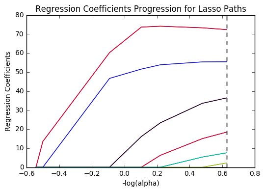
Plot coefficient progression

In [12]:m_log_alphas =-np.log10(model.alphas_) ax = plt.gca() plt.plot(m_log_alphas, model.coef_path_.T) plt.axvline(-np.log10(model.alpha_), linestyle='--', color='k', label='alpha CV') plt.ylabel('Regression Coefficients') plt.xlabel('-log(alpha)') plt.title('Regression Coefficients Progression for Lasso Paths') plt.show()

Plot mean square error for each fold

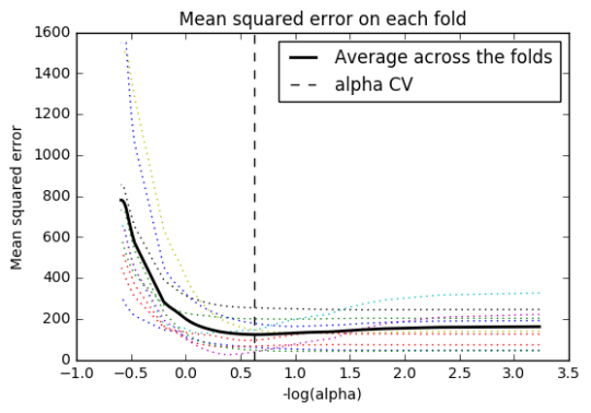
In [13]:m_log_alphascv =-np.log10(model.cv_alphas_) plt.figure() plt.plot(m_log_alphascv, model.cv_mse_path_, ':') plt.plot(m_log_alphascv, model.cv_mse_path_.mean(axis=-1), 'k', label='Average across the folds', linewidth=2) plt.axvline(-np.log10(model.alpha_), linestyle='--', color='k', label='alpha CV') plt.legend() plt.xlabel('-log(alpha)') plt.ylabel('Mean squared error') plt.title('Mean squared error on each fold') plt.show()

Print the mean squared error from training and test data

In [17]:from sklearn.metrics import mean_squared_error train_error = mean_squared_error(tar_train, model.predict(pred_train)) test_error = mean_squared_error(tar_test, model.predict(pred_test)) print ('training data MSE') print(train_error) print ('') print ('test data MSE') print(test_error) training data MSE 100.103936002 test data MSE 120.568970231

Print the r-squared from training and test data

In [18]:rsquared_train=model.score(pred_train,tar_train) rsquared_test=model.score(pred_test,tar_test) print ('training data R-square') print(rsquared_train) print ('') print ('test data R-square') print(rsquared_test) training data R-square 0.861344142378 test data R-square 0.776942580854

Data were randomly split into a training set that included 70% of the observations (N=42) and a test set that included 30% of the observations (N=18). The least angle regression algorithm with k=10 fold cross validation was used to estimate the lasso regression model in the training set, and the model was validated using the test set. The change in the cross validation average (mean) squared error at each step was used to identify the best subset of predictor variables.

Of the 10 predictor variables, 6 were retained in the model. During the estimation process, income per person and life expectancy were most strongly associated with internet use rate, followed by alcohol consumption and electricity use per person. The last two predictors were urban rate and polity score. All variables were positively correlated with internet use rate. These 6 variables accounted for 77.7% of the variance in the internet use rate response variable.

[machine-learning-coursera]

Machine Learning for Data Analysis

Week 2: Running a Random Forest

The main drawback to a decision tree is that the tree is highly specific to the dataset it was built on; if you bring in new data to try and predict outcomes, you may not find the same high correlations that your decision tree featured. One method to overcome this is with a random forest. Instead of building one tree from your whole dataset, you subset the data randomly and build a number of trees. Each tree will be different, but the relationships between your variables will tend to appear consistently. In general though, because decision trees are intrinsically connected to the specific data they were built with, decision trees are better as a tool to analyze trends within a known dataset than to create a model for predicting the outcomes of future data.

With those caveats, I decided to build a random forest using the same data as from my previous post, that is, a response variable of internet use rate and explanatory variables of income per person, employment rate, female employment rate, and polity score, from the GapMinder dataset.

Load the data, convert the variables to numeric, convert the response variable to binary, and remove NA values.

In [3]: import pandas as pd import numpy as np import matplotlib.pyplot as plt from sklearn.cross_validation import train_test_split import sklearn.metrics from sklearn.ensemble import ExtraTreesClassifier data = pd.read_csv('c:/users/greg/desktop/gapminder.csv', low_memory=False) data['internetuserate'] = pd.to_numeric(data['internetuserate'], errors='coerce') data['incomeperperson'] = pd.to_numeric(data['incomeperperson'], errors='coerce') data['employrate'] = pd.to_numeric(data['employrate'], errors='coerce') data['femaleemployrate'] = pd.to_numeric(data['femaleemployrate'], errors='coerce') data['polityscore'] = pd.to_numeric(data['polityscore'], errors='coerce') binarydata = data.copy() # convert response variable to binarydef internetgrp (row): if row['internetuserate'] < data['internetuserate'].median(): return 0 else: return 1 binarydata['internetuserate'] = binarydata.apply (lambda row: internetgrp (row),axis=1) # Clean the dataset binarydata_clean = binarydata.dropna()

Build the model from the training set

In [10]:predictors = binarydata_clean[['incomeperperson','employrate','femaleemployrate','polityscore']] targets = binarydata_clean.internetuserate pred_train, pred_test, tar_train, tar_test = train_test_split(predictors, targets, test_size=.4) from sklearn.ensemble import RandomForestClassifier classifier_r=RandomForestClassifier(n_estimators=25) classifier_r=classifier_r.fit(pred_train,tar_train) predictions_r=classifier_r.predict(pred_test)

Print the confusion matrix

In [11]:sklearn.metrics.confusion_matrix(tar_test,predictions_r)

Out[11]:array([[22, 5], [10, 24]])

Print the accuracy score

In [12]:sklearn.metrics.accuracy_score(tar_test, predictions_r)

Out[12]:0.75409836065573765

Fit an Extra Trees model to the data

In [13]:model_r = ExtraTreesClassifier() model_r.fit(pred_train,tar_train)

Out[13]:ExtraTreesClassifier(bootstrap=False, class_weight=None, criterion='gini', max_depth=None, max_features='auto', max_leaf_nodes=None, min_samples_leaf=1, min_samples_split=2, min_weight_fraction_leaf=0.0, n_estimators=10, n_jobs=1, oob_score=False, random_state=None, verbose=0, warm_start=False)

Display the Relative Importances of Each Attribute

In [15]:model_r.feature_importances_

Out[15]:array([ 0.44072852, 0.12553198, 0.1665162 , 0.2672233 ])

Run a different number of trees and see the effect of that on the accuracy of the prediction

In [16]:trees=range(50) accuracy=np.zeros(50) for idx in range(len(trees)): classifier_r=RandomForestClassifier(n_estimators=idx + 1) classifier_r=classifier_r.fit(pred_train,tar_train) predictions_r=classifier_r.predict(pred_test) accuracy[idx]=sklearn.metrics.accuracy_score(tar_test, predictions_r) plt.cla() plt.plot(trees, accuracy) plt.ylabel('Accuracy Score') plt.xlabel('Number of Trees') plt.show()

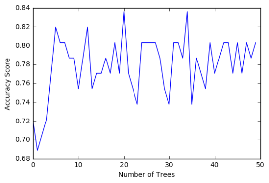
The confusion matrix and accuracy score are similar to that of my previous post (remember, a decision tree is pseudo-randomly created, so results will be similar, but not identical, when run with the same dataset). Examining the relative importance of each attribute is interesting here. As expected, income per person is the most highly correlated with internet use rate, at 54% of the model’s predictive capability. Employment rate (15%) and female employment rate (11%) are less correlated, again, as expected. But polity score, at 20% of the model’s predictive capability, stood out to me because none of the previous models I’ve examined with this dataset have had polity score even near the same level of importance as employment rates. Interesting. Finally, the graph shows that as the number of trees in the forest grows, the accuracy of the model does as well, but only up to about 20 trees. After that, the accuracy stops increasing and instead fluctuates with the random permutations of the subsets of data that were used to create the trees.

[machine-learning-coursera]

Week 1 : Running a Classification Tree

For the next few posts, I’ll be exploring machine learning techniques to help analyze the GapMinder data. To begin, I’ll create a classification tree to explore the relationship between my response variable, internet user rate, and my explanatory variables, income per person, employment rate, female employment rate, and polity score. The technique requires a binary, categorical response variable, so for the purpose of this demonstration I have binned internet use rate into two categories, High usage and Low usage, split by the median data point.

Load the data and convert the variables to numeric

import pandas as pd from sklearn.cross_validation import train_test_split from sklearn.tree import DecisionTreeClassifier import sklearn.metrics data = pd.read_csv('c:/users/greg/desktop/gapminder.csv', low_memory=False) data['internetuserate'] = pd.to_numeric(data['internetuserate'], errors='coerce') data['incomeperperson'] = pd.to_numeric(data['incomeperperson'], errors='coerce') data['employrate'] = pd.to_numeric(data['employrate'], errors='coerce') data['femaleemployrate'] = pd.to_numeric(data['femaleemployrate'], errors='coerce') data['polityscore'] = pd.to_numeric(data['polityscore'], errors='coerce')

Convert the response variable to binary

binarydata = data.copy() def internetgrp (row): if row['internetuserate'] < data['internetuserate'].median(): return 0 else: return 1 binarydata['internetuserate'] = binarydata.apply (lambda row: internetgrp (row),axis=1)

Clean the data by discarding NA values

In [4]:binarydata_clean = binarydata.dropna() binarydata_clean.dtypes binarydata_clean.describe()

Out[4]:incomeperpersonfemaleemployrateinternetuseratepolityscoreemployratecount152.000000152.000000152.000000152.000000152.000000mean6706.55697848.0684210.4539473.86184259.212500std9823.59231514.8268570.4995216.24558110.363802min103.77585712.4000000.000000-10.00000034.90000225%560.79715839.5499990.000000-2.00000051.92499950%2225.93101948.5499990.0000007.00000058.90000275%6905.28766256.0500001.0000009.00000065.000000max39972.35276883.3000031.00000010.00000083.199997

Split into training and testing sets

In [7]:predictors = binarydata_clean[['incomeperperson','employrate','femaleemployrate','polityscore']] targets = binarydata_clean.internetuserate pred_train, pred_test, tar_train, tar_test = train_test_split(predictors, targets, test_size=.4) print ('Training sample') print (pred_train.shape) print ('') print ('Testing sample') print (pred_test.shape) print ('') print ('Training sample') print (tar_train.shape) print ('') print ('Testing sample') print (tar_test.shape) Training sample (91, 4) Testing sample (61, 4) Training sample (91,) Testing sample (61,)

Build model on the training data

In [8]:classifier=DecisionTreeClassifier() classifier=classifier.fit(pred_train,tar_train) predictions=classifier.predict(pred_test)

Display the confusion matrix

In [10]:sklearn.metrics.confusion_matrix(tar_test,predictions)

Out[10]:array([[22, 9], [ 8, 22]])

Display the accuracy score

In [11]:sklearn.metrics.accuracy_score(tar_test, predictions)

Out[11]:0.72131147540983609

Display the decision tree

In [13]:from sklearn import tree from io import StringIO from IPython.display import Image out = StringIO() tree.export_graphviz(classifier, out_file=out) import pydotplus graph=pydotplus.graph_from_dot_data(out.getvalue()) Image(graph.create_png())

Out[13]:

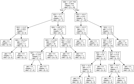
The decision tree analysis was performed to test non-linear relationships among the explanatory variables and a single binary, categorical response variable. The training sample has 91 rows of data and 4 explanatory variables; the testing sample has 61 rows of data, and the same 4 explanatory variables. The decision tree results in 27 true negatives and 16 true positives; and 11 false negatives and 7 false positives. The accuracy score is 70.5%, meaning that the model accurately predicted 70.5% of the internet use rates per country.