machine-learning-da

[machine-learning-da]

k-means Cluster Analysis

A k-means cluster analysis was conducted to identify underlying subgroups of adolescents based on their similarity of responses on 11 variables that represent characteristics that could have an impact on school achievement. Clustering variables included two binary variables measuring whether or not the adolescent had ever used alcohol or marijuana, as well as quantitative variables measuring alcohol problems, a scale measuring engaging in deviant behaviours (such as vandalism, other property damage, lying, stealing, running away, driving without permission, selling drugs, and skipping school), and scales measuring violence, depression, self-esteem, parental presence, parental activities, family connectedness, and school connectedness.

 To build a k-mans clustering model we perform the following steps. We import all the necessary libraries. We import the dataset and also clean the data.  we will create a data set called cluster that includes only our clustering variables.

In cluster analysis variables with large values contribute more to the distance calculations.Variables measured on different scales should be standardized prior to clustering, so that the solution is not driven by variables measured on larger scales. We use the following code to standardize the clustering variables to have a mean of 0, and a standard deviation of 1. 

clustervar['ALCEVR1']=preprocessing.scale(clustervar['ALCEVR1'].astype('float64'))

clustervar['ALCPROBS1']=preprocessing.scale(clustervar['ALCPROBS1'].astype('float64'))

clustervar['MAREVER1']=preprocessing.scale(clustervar['MAREVER1'].astype('float64'))

clustervar['DEP1']=preprocessing.scale(clustervar['DEP1'].astype('float64'))

clustervar['ESTEEM1']=preprocessing.scale(clustervar['ESTEEM1'].astype('float64'))

clustervar['VIOL1']=preprocessing.scale(clustervar['VIOL1'].astype('float64'))

clustervar['DEVIANT1']=preprocessing.scale(clustervar['DEVIANT1'].astype('float64'))

clustervar['FAMCONCT']=preprocessing.scale(clustervar['FAMCONCT'].astype('float64'))

clustervar['SCHCONN1']=preprocessing.scale(clustervar['SCHCONN1'].astype('float64'))

clustervar['PARACTV']=preprocessing.scale(clustervar['PARACTV'].astype('float64'))

clustervar['PARPRES']=preprocessing.scale(clustervar['PARPRES'].astype('float64')) 

We then train the data set using the train_test_split function which randomly split the data into training set and test set. Before cluster analysing we need to know the values of k this is achieved using the following code. The for k in clusters: code tells Python to run the cluster analysis code below for each value of k in the cluster's object. 

 from scipy.spatial.distance import cdist

clusters=range(1,10)

meandist=[]. 

After we have the average distance calculated for each of the 1 to 9 cluster solutions we can plot the elbow curve using the map plot lib plot function that we imported as plt.

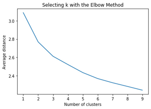
 This plot shows the decrease in the average minimum distance of the observations from the cluster centroids for each of the cluster solutions. We can see that the average distance decreases as the number of clusters increases. Since the goal of cluster analysis is to minimize the distance between observations and their assigned clusters, we want to choose the fewest numbers of clusters that provides a low average distance. What we're looking for in this plot is a bend in the elbow that kind of shows where the average distance value might be levelling off such that adding more clusters doesn't decrease the average distance as much.  

Since we can see a bend at 3 we rerun the cluster analysis, this time asking for 3 clusters. So we create an object, model 3, which will contain the results from the cluster analysis with 3 clusters =KMeans, and in parenthesis, n_clusters=3. And we fit the model and create an object called clusassign that has the cluster assignments based on the 3 cluster model. we're going to use is use canonical discriminate analysis, which is a data reduction technique that creates a smaller number of variables that are linear combinations of the clustering variables mentioned. The new variables, called canonical variables, are ordered in terms of the proportion of variance and the clustering variables that is accounted for by each of the canonical variables. In Python, we can use the PCA function and the sklearn decomposition library to conduct the canonical discriminate analysis.We will plot the two canonical variables by the cluster assignment values from the 3 cluster solution in a scatter plot using the matplot libplot function.

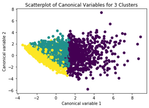
Here is the scatter plot. What this shows is that these two clusters are densely packed, meaning that the observations within the clusters are pretty highly correlated with each other, and within cluster variance is relatively low. The left part of the plot appear to have a good deal of overlap, meaning that there is not good separation between these two clusters. On the other hand, this cluster here shows better separation, but the observations are more spread out indicating less correlation among the observations and higher within cluster variance.This suggests that the two cluster solution might be better, meaning that it would be especially important to further evaluate the two cluster solution as well.  we can take a look at the pattern of means on the clustering variables for each cluster to see whether they are distinct and meaningful. To do this, we have to link the cluster assignment variable back to its corresponding observation in the clus_train dataset that has the clustering variables.  

Multiple steps to merge cluster assignment with clustering variables to examine cluster variable means by cluster. Create a unique identifier variable from the index for the cluster training data to merge with the cluster assignment variable. Then create a list that has the new index variable and create a list of cluster assignments. Combine index variable list with cluster assignment list into a dictionary. Convert newlist dictionary to a dataframe and rename the cluster assignment column. Cow do the same for the cluster assignment variablecreate a unique identifier variable from the index for the cluster assignment dataframe to merge with cluster training data, then merge the cluster assignment dataframe with the cluster training variable dataframe by the index variable. Merge cluster assignment with clustering variables to examine cluster variable means by cluster. Finaly calculate clustering variable means by cluster by using group by.

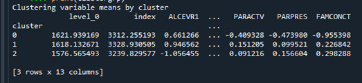
The means on the clustering variables showed that compared to the other clusters, adolescents in the first cluster, cluster 0, had the highest likelihood of having used alcohol, but otherwise tended to fall somewhere in between the other two clusters on the other variables. On the other hand, the second cluster, cluster 1, clearly includes the most troubled adolescents. Adolescents in this cluster had the highest likelihood of having used alcohol, a very high likelihood of having used marijuana, more alcohol problems, and more engagement in deviant and violent behaviors compared to the other two clusters. They also had higher levels of depression, lower self-steem, and the lowest levels of school connectedness, parental presence, involvement of parent in activities, and family connectedness. The third cluster, cluster 2, appears to include the least troubled adolescents. Compared to adolescents in the other clusters, they were least likely to have used alcohol and marijuana, and had the lowest number of alcohol problems and deviant and violent behavior. They also had greater school and family connectedness. 

Validate clusters in training data by examining cluster differences in GPA using ANOVA. have to merge GPA with clustering variables and cluster assignment data. Then split the GPA data for training and testing.  We then print the mean GPA in standard deviation for each cluster using the groupby function.

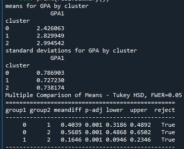
The analysis of variance summary table indicates that the clusters differed significantly on GPA. When we examine the means, we find that not surprisingly, adolescents in cluster 1, the most troubled group, had the lowest GPA, and adolescents in cluster 2, the least troubled group, had the highest GPA. The tukey test shows that the clusters differed significantly in mean GPA, although the difference between cluster 0 and cluster 2 were smaller. 

The full code for cluster analysis is as follows:   

from pandas import Series, DataFrame

import pandas as pd

import numpy as np

import matplotlib.pylab as plt

from sklearn.model_selection import train_test_split

from sklearn import preprocessing

from sklearn.cluster import KMeans

data = pd.read_csv("tree_addhealth.csv")

data.columns = map(str.upper, data.columns) 

data_clean = data.dropna()

 # subset clustering variables

cluster=data_clean[['ALCEVR1','MAREVER1','ALCPROBS1','DEVIANT1','VIOL1',

'DEP1','ESTEEM1','SCHCONN1','PARACTV', 'PARPRES','FAMCONCT']]

cluster.describe()

 # standardize clustering variables to have mean=0 and sd=1

clustervar=cluster.copy()

clustervar['ALCEVR1']=preprocessing.scale(clustervar['ALCEVR1'].astype('float64'))

clustervar['ALCPROBS1']=preprocessing.scale(clustervar['ALCPROBS1'].astype('float64'))

clustervar['MAREVER1']=preprocessing.scale(clustervar['MAREVER1'].astype('float64'))

clustervar['DEP1']=preprocessing.scale(clustervar['DEP1'].astype('float64'))

clustervar['ESTEEM1']=preprocessing.scale(clustervar['ESTEEM1'].astype('float64'))

clustervar['VIOL1']=preprocessing.scale(clustervar['VIOL1'].astype('float64'))

clustervar['DEVIANT1']=preprocessing.scale(clustervar['DEVIANT1'].astype('float64'))

clustervar['FAMCONCT']=preprocessing.scale(clustervar['FAMCONCT'].astype('float64'))

clustervar['SCHCONN1']=preprocessing.scale(clustervar['SCHCONN1'].astype('float64'))

clustervar['PARACTV']=preprocessing.scale(clustervar['PARACTV'].astype('float64'))

clustervar['PARPRES']=preprocessing.scale(clustervar['PARPRES'].astype('float64'))

 # split data into train and test sets

clus_train, clus_test = train_test_split(clustervar, test_size=.3, random_state=123)

 # k-means cluster analysis for 1-9 clusters                                                          

from scipy.spatial.distance import cdist

clusters=range(1,10)

meandist=[]

 for k in clusters:

   model=KMeans(n_clusters=k)

   model.fit(clus_train)

   clusassign=model.predict(clus_train)

  meandist.append(sum(np.min(cdist(clus_train, model.cluster_centers_, 'euclidean'), axis=1))

   / clus_train.shape[0])

plt.plot(clusters, meandist)

plt.xlabel('Number of clusters')

plt.ylabel('Average distance')

plt.title('Selecting k with the Elbow Method')

 # Interpret 3 cluster solution

model3=KMeans(n_clusters=3)

model3.fit(clus_train)

clusassign=model3.predict(clus_train)

# plot clusters

 from sklearn.decomposition import PCA

pca_2 = PCA(2)

plot_columns = pca_2.fit_transform(clus_train)

plt.scatter(x=plot_columns[:,0], y=plot_columns[:,1], c=model3.labels_,)

plt.xlabel('Canonical variable 1')

plt.ylabel('Canonical variable 2')

plt.title('Scatterplot of Canonical Variables for 3 Clusters')

plt.show()

clus_train.reset_index(level=0, inplace=True)

cluslist=list(clus_train['index'])

labels=list(model3.labels_)

newlist=dict(zip(cluslist, labels))

newlist

newclus=DataFrame.from_dict(newlist, orient='index')

newclus

newclus.columns = ['cluster']

newclus.reset_index(level=0, inplace=True)

merged_train=pd.merge(clus_train, newclus, on='index')

merged_train.head(n=100)

merged_train.cluster.value_counts()

clustergrp = merged_train.groupby('cluster').mean()

print ("Clustering variable means by cluster")

print(clustergrp)

 gpa_data=data_clean['GPA1']

gpa_train, gpa_test = train_test_split(gpa_data, test_size=.3, random_state=123)

gpa_train1=pd.DataFrame(gpa_train)

gpa_train1.reset_index(level=0, inplace=True)

merged_train_all=pd.merge(gpa_train1, merged_train, on='index')

sub1 = merged_train_all[['GPA1', 'cluster']].dropna()

 import statsmodels.formula.api as smf

import statsmodels.stats.multicomp as multi

 gpamod = smf.ols(formula='GPA1 ~ C(cluster)', data=sub1).fit()

print (gpamod.summary())

 print ('means for GPA by cluster')

m1= sub1.groupby('cluster').mean()

print (m1)

 print ('standard deviations for GPA by cluster')

m2= sub1.groupby('cluster').std()

print (m2)

 mc1 = multi.MultiComparison(sub1['GPA1'], sub1['cluster'])

res1 = mc1.tukeyhsd()

print(res1.summary())

[machine-learning-da]

Lasso Regression Analysis

A lasso regression analysis was conducted to identify a subset of variables from a pool of 23 categorical and quantitative predictor variables that best predicted a quantitative response variable measuring school connectedness in adolescents. Categorical predictors included gender and a series of 5 binary categorical variables for race and ethnicity (Hispanic, White, Black, Native American and Asian) to improve interpretability of the selected model with fewer predictors. Binary substance use variables were measured with individual questions about whether the adolescent had ever used alcohol, marijuana, cocaine or inhalants. Additional categorical variables included the availability of cigarettes in the home, whether or not either parent was on public assistance and any experience with being expelled from school. Quantitative predictor variables include age, alcohol problems, and a measure of deviance that included such behaviors as vandalism, other property damage, lying, stealing, running away, driving without permission, selling drugs, and skipping school. Another scale for violence, one for depression, and others measuring self-esteem, parental presence, parental activities, family connectedness and grade point average were also included. All predictor variables were standardized to have a mean of zero and a standard deviation of one.

 In lasso regression, the penalty term is not fair if the predictive variables are not on the same scale, meaning that not all the predictors get the same penalty. So all predicters should be standardized to have a mean equal to zero and a standard deviation equal to one, including my binary predictors. It is done as follows

  # standardize predictors to have mean=0 and sd=1

predictors=predvar.copy()

from sklearn import preprocessing

predictors['MALE']=preprocessing.scale(predictors['MALE'].astype('float64'))

predictors['HISPANIC']=preprocessing.scale(predictors['HISPANIC'].astype('float64'))

predictors['WHITE']=preprocessing.scale(predictors['WHITE'].astype('float64'))

predictors['NAMERICAN']=preprocessing.scale(predictors['NAMERICAN'].astype('float64'))

predictors['ASIAN']=preprocessing.scale(predictors['ASIAN'].astype('float64'))

predictors['AGE']=preprocessing.scale(predictors['AGE'].astype('float64'))

predictors['ALCEVR1']=preprocessing.scale(predictors['ALCEVR1'].astype('float64'))

predictors['ALCPROBS1']=preprocessing.scale(predictors['ALCPROBS1'].astype('float64'))

predictors['MAREVER1']=preprocessing.scale(predictors['MAREVER1'].astype('float64'))

predictors['COCEVER1']=preprocessing.scale(predictors['COCEVER1'].astype('float64'))

predictors['INHEVER1']=preprocessing.scale(predictors['INHEVER1'].astype('float64'))

predictors['CIGAVAIL']=preprocessing.scale(predictors['CIGAVAIL'].astype('float64'))

predictors['DEP1']=preprocessing.scale(predictors['DEP1'].astype('float64'))

predictors['ESTEEM1']=preprocessing.scale(predictors['ESTEEM1'].astype('float64'))

predictors['VIOL1']=preprocessing.scale(predictors['VIOL1'].astype('float64'))

predictors['PASSIST']=preprocessing.scale(predictors['PASSIST'].astype('float64'))

predictors['DEVIANT1']=preprocessing.scale(predictors['DEVIANT1'].astype('float64'))

predictors['GPA1']=preprocessing.scale(predictors['GPA1'].astype('float64'))

predictors['EXPEL1']=preprocessing.scale(predictors['EXPEL1'].astype('float64'))

predictors['FAMCONCT']=preprocessing.scale(predictors['FAMCONCT'].astype('float64'))

predictors['PARACTV']=preprocessing.scale(predictors['PARACTV'].astype('float64'))

predictors['PARPRES']=preprocessing.scale(predictors['PARPRES'].astype('float64'))

  Data is split into a training set that included 70% of the observations (N=3201) and a test set that included 30% of the observations (N=1701).

 to run our LASSO regression analysis with the LAR algorithm using the LASSO LarsCV function from the sklearn linear model library we type the following code.

 model=LassoLarsCV(cv=10, precompute=False).fit(pred_train,tar_train)

   LAR Algorithm was used which stands for Least Angle Regression. This algorithm starts with no predictors in the model and adds a predictor at each step. It first adds a predictor that is most correlated with the response variable and moves it towards least score estimate until there is another predictor. That is equally correlated with the model residual. It adds this predictor to the model and starts the least square estimation process over again with both variables. The LAR algorithm continues with this process until it has tested all the predictors. Parameter estimates at any step are shrunk and predictors with coefficients that have shrunk to zero are removed from the model and the process starts all over again. The model that produces the lowest mean-square error is selected by Python as the best model to validate using the test data set.

 The least angle regression algorithm with k=10-fold cross validation was used to estimate the lasso regression model in the training set, and the model was validated using the test set. The change in the cross-validation average (mean) squared error at each step was used to identify the best subset of predictor variables. The precompute matrix is set to false as the dataset is not very large.

 The dict object creates a dictionary, and the zip object creates lists. Output is as follows:

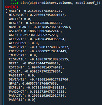
Predictors with regression coefficients equal to zero means that the coefficients for those variables had shrunk to zero after applying the LASSO regression penalty, and were subsequently removed from the model. So the results show that of the 23 variables, 18 were selected in the final model 18 were selected in the final model.

We can also create some plots so we can visualize some of the results. We can plot the progression of the regression coefficients through the model selection process.In Python, we do this by plotting the change in the regression coefficient by values of penalty parameter at each step of selection process. We can use the following code to generate this plot.

This plot shows the relative importance of the predictor selected at any step of the selection process, how the regression coefficients changed with the addition of a new predictor at each step, as well as the steps at which each variable entered the model. As we already know from looking at the list of the regression coefficients self esteem, the dark blue line, had the largest regression coefficient. It was therefore entered into the model first, followed by depression, the black line, at step two. In black ethnicity, the light blue line, at step three and so on.

 Another important plot is one that shows the change in the mean square error for the change in the penalty parameter alpha at each step in the selection process. This code is similar to the code for the previous plot except this time we're plotting the alpha values through the model selection process for each cross-validation fold on the horizontal axis, and the mean square error for each cross validation fold on vertical axis.

We can see that there is variability across the individual cross-validation folds in the training data set, but the change in the mean square error as variables are added to the model follows the same pattern for each fold. Initially it decreases rapidly and then levels off to a point at which adding more predictors doesn't lead to much reduction in the mean square error. This is to be expected as model complexity increases.

 We can also print the average mean square error in the r square for the proportion of variance in school connectedness.

The R-square values were 0.33 and 0.31, indicating that the selected model explained 33 and 31% of the variance in school connectedness for the training and test sets, respectively.

 The full code is as follows:

 #from pandas import Series, DataFrame

import pandas as pd

import numpy as np

import matplotlib.pylab as plt

from sklearn.model_selection import train_test_split

from sklearn.linear_model import LassoLarsCV

#Load the dataset

data = pd.read_csv("tree_addhealth.csv")

 #upper-case all DataFrame column names

data.columns = map(str.upper, data.columns)

 # Data Management

data_clean = data.dropna()

recode1 = {1:1, 2:0}

data_clean['MALE']= data_clean['BIO_SEX'].map(recode1)

 #select predictor variables and target variable as separate data sets  

predvar= data_clean[['MALE','HISPANIC','WHITE','BLACK','NAMERICAN','ASIAN',

'AGE','ALCEVR1','ALCPROBS1','MAREVER1','COCEVER1','INHEVER1','CIGAVAIL','DEP1',

'ESTEEM1','VIOL1','PASSIST','DEVIANT1','GPA1','EXPEL1','FAMCONCT','PARACTV',

'PARPRES']]

 target = data_clean.SCHCONN1

# standardize predictors to have mean=0 and sd=1

predictors=predvar.copy()

from sklearn import preprocessing

predictors['MALE']=preprocessing.scale(predictors['MALE'].astype('float64'))

predictors['HISPANIC']=preprocessing.scale(predictors['HISPANIC'].astype('float64'))

predictors['WHITE']=preprocessing.scale(predictors['WHITE'].astype('float64'))

predictors['NAMERICAN']=preprocessing.scale(predictors['NAMERICAN'].astype('float64'))

predictors['ASIAN']=preprocessing.scale(predictors['ASIAN'].astype('float64'))

predictors['AGE']=preprocessing.scale(predictors['AGE'].astype('float64'))

predictors['ALCEVR1']=preprocessing.scale(predictors['ALCEVR1'].astype('float64'))

predictors['ALCPROBS1']=preprocessing.scale(predictors['ALCPROBS1'].astype('float64'))

predictors['MAREVER1']=preprocessing.scale(predictors['MAREVER1'].astype('float64'))

predictors['COCEVER1']=preprocessing.scale(predictors['COCEVER1'].astype('float64'))

predictors['INHEVER1']=preprocessing.scale(predictors['INHEVER1'].astype('float64'))

predictors['CIGAVAIL']=preprocessing.scale(predictors['CIGAVAIL'].astype('float64'))

predictors['DEP1']=preprocessing.scale(predictors['DEP1'].astype('float64'))

predictors['ESTEEM1']=preprocessing.scale(predictors['ESTEEM1'].astype('float64'))

predictors['VIOL1']=preprocessing.scale(predictors['VIOL1'].astype('float64'))

predictors['PASSIST']=preprocessing.scale(predictors['PASSIST'].astype('float64'))

predictors['DEVIANT1']=preprocessing.scale(predictors['DEVIANT1'].astype('float64'))

predictors['GPA1']=preprocessing.scale(predictors['GPA1'].astype('float64'))

predictors['EXPEL1']=preprocessing.scale(predictors['EXPEL1'].astype('float64'))

predictors['FAMCONCT']=preprocessing.scale(predictors['FAMCONCT'].astype('float64'))

predictors['PARACTV']=preprocessing.scale(predictors['PARACTV'].astype('float64'))

predictors['PARPRES']=preprocessing.scale(predictors['PARPRES'].astype('float64'))

 # split data into train and test sets

pred_train, pred_test, tar_train, tar_test = train_test_split(predictors, target,

                                                            test_size=.3, random_state=123)

 # specify the lasso regression model

model=LassoLarsCV(cv=10, precompute=False).fit(pred_train,tar_train)

 # print variable names and regression coefficients

dict(zip(predictors.columns, model.coef_))

 # plot coefficient progression

m_log_alphas = -np.log10(model.alphas_)

ax = plt.gca()

plt.plot(m_log_alphas, model.coef_path_.T)

plt.axvline(-np.log10(model.alpha_), linestyle='--', color='k',

           label='alpha CV')

plt.ylabel('Regression Coefficients')

plt.xlabel('-log(alpha)')

plt.title('Regression Coefficients Progression for Lasso Paths')

 # plot mean square error for each fold

m_log_alphascv = -np.log10(model.cv_alphas_)

plt.figure()

plt.plot(m_log_alphascv, model.cv_mse_path_, ':')

plt.plot(m_log_alphascv, model.cv_mse_path_.mean(axis=-1), 'k',

        label='Average across the folds', linewidth=2)

plt.axvline(-np.log10(model.alpha_), linestyle='--', color='k',

           label='alpha CV')

plt.legend()

plt.xlabel('-log(alpha)')

plt.ylabel('Mean squared error')

plt.title('Mean squared error on each fold')

         # MSE from training and test data

from sklearn.metrics import mean_squared_error

train_error = mean_squared_error(tar_train, model.predict(pred_train))

test_error = mean_squared_error(tar_test, model.predict(pred_test))

print ('training data MSE')

print(train_error)

print ('test data MSE')

print(test_error)

 # R-square from training and test data

rsquared_train=model.score(pred_train,tar_train)

rsquared_test=model.score(pred_test,tar_test)

print ('training data R-square')

print(rsquared_train)

print ('test data R-square')

print(rsquared_test)

[machine-learning-da]

Random Forest

The diagonal values 1432 and 116 show the number of true negative and true positive classification. 199 shows the false negative and 83 show false positive.

We can also see the accuracy which shows 0.84, which means 84% of people are regular smokers.

Random forest analysis was performed to evaluate the importance of a series of explanatory variables in predicting a binary, categorical response variable. The following explanatory variables were included as possible contributors to a random forest evaluating regular smoking (my response variable), age, gender, (race/ethnicity) Hispanic, White, Black, Native American and Asian. Alcohol use, marijuana use, cocaine use, inhalant use, availability of cigarettes in the home, whether or not either parent was on public assistance, any experience with being expelled from school, alcohol problems, deviance, violence, depression, self-esteem, parental presence, parental activities, family connectedness, school connectedness and grade point average.

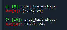
Like in classification trees  get to know the shape of the training and test data set. We can see that training sample has 2745 observation, that is 60% of the sample given and 24 explanatory variables and test sample has 1830 observation, that is 40% of the sample given and 24 explanatory variables.

 We also have confusion matrix. Showing the correct and incorrect classification.

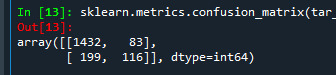
The diagonal values 1432 and 116 show the number of true negative and true positive classification. 199 shows the false negative and 83 show false positive.

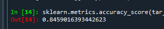
We can also see the accuracy which shows 0.84, which means 84% of people are regular smokers.

Given that we don't interpret individual trees in a random forest, the most helpful information to be gotten from a forest is arguably the measured importance for each explanatory variable. 

Also called the features. 

Based on how many votes or splits each has produced in the 25 tree ensemble. To generate importance scores, we initialize the extra tree classifier, and then fit a model.

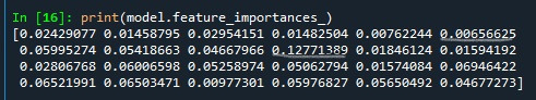
 Following shows the feature important scores. The variables are listed in the order they've been named earlier in the code. Starting with gender, called BIO_SEX, and ending with parental presence. As we can see the variables with the highest important score at 0.127 is marijuana use. And the variable with the lowest important score is Asian ethnicity at .006.

Code for building random forest classifier from 1 to 25 nd finding accuracy for those trees.

 trees=range(25)

accuracy=np.zeros(25)

for idx in range(len(trees)):

  classifier=RandomForestClassifier(n_estimators=idx + 1)

  classifier=classifier.fit(pred_train,tar_train)

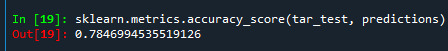
  predictions=classifier.predict(pred_test)

  accuracy[idx]=sklearn.metrics.accuracy_score(tar_test, predictions)

 And we'll plot them as the number of trees increase.

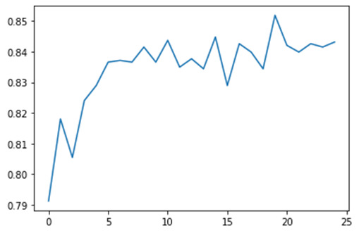
As you can see there is one tree with 82% accuracy and it climbs to only about 85% with successive trees that are grown giving us some confidence that it may be perfectly appropriate to interpret a single decision tree for this data.

The full code is as follows:

from pandas import Series, DataFrame

import pandas as pd

import numpy as np

import os

import matplotlib.pylab as plt

from sklearn.model_selection import train_test_split

from sklearn.tree import DecisionTreeClassifier

from sklearn.metrics import classification_report

import sklearn.metrics

# Feature Importance

from sklearn import datasets

from sklearn.ensemble import ExtraTreesClassifier

   #Load the dataset

 AH_data = pd.read_csv("tree_addhealth.csv")

data_clean = AH_data.dropna()

 data_clean.dtypes

data_clean.describe()

 #Split into training and testing sets

 predictors = data_clean[['BIO_SEX','HISPANIC','WHITE','BLACK','NAMERICAN','ASIAN','age',

'ALCEVR1','ALCPROBS1','marever1','cocever1','inhever1','cigavail','DEP1','ESTEEM1','VIOL1',

'PASSIST','DEVIANT1','SCHCONN1','GPA1','EXPEL1','FAMCONCT','PARACTV','PARPRES']]

 targets = data_clean.TREG1

 pred_train, pred_test, tar_train, tar_test  = train_test_split(predictors, targets, test_size=.4)

 pred_train.shape

pred_test.shape

tar_train.shape

tar_test.shape

 #Build model on training data

from sklearn.ensemble import RandomForestClassifier

 classifier=RandomForestClassifier(n_estimators=25)

classifier=classifier.fit(pred_train,tar_train)

 predictions=classifier.predict(pred_test)

 sklearn.metrics.confusion_matrix(tar_test,predictions)

sklearn.metrics.accuracy_score(tar_test, predictions)

  # fit an Extra Trees model to the data

model = ExtraTreesClassifier()

model.fit(pred_train,tar_train)

# display the relative importance of each attribute

print(model.feature_importances_)

  """

Running a different number of trees and see the effect

of that on the accuracy of the prediction

"""

 trees=range(25)

accuracy=np.zeros(25)

 for idx in range(len(trees)):

  classifier=RandomForestClassifier(n_estimators=idx + 1)

  classifier=classifier.fit(pred_train,tar_train)

  predictions=classifier.predict(pred_test)

  accuracy[idx]=sklearn.metrics.accuracy_score(tar_test, predictions)

  plt.cla()

plt.plot(trees, accuracy)

[machine-learning-da]

Run a Classification Tree.

Decision tree analysis was performed to test nonlinear relationships among a series of explanatory variables and a binary, categorical response variable. All possible separations (categorical) or cut points (quantitative) are tested. For the present analyses, the entropy “goodness of split” criterion was used to grow the tree and a cost complexity algorithm was used for pruning the full tree into a final subtree.

The following explanatory variables were included as possible contributors to a classification tree model evaluating smoking experimentation (my response variable), age, gender, (race/ethnicity) Hispanic, White, Black, Native American and Asian. Alcohol use, marijuana use, cocaine use, inhalant use, availability of cigarettes in the home, whether or not either parent was on public assistance, any experience with being expelled from school. alcohol problems, deviance, violence, depression, self-esteem, parental presence, parental activities, family connectedness, school connectedness and grade point average.

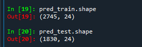
We can also get to know the shape of the training and test data set. We can see that training sample has 2745 observation, that is 60% of the sample given and 24 explanatory variables and test sample has 1830 observation, that is 40% of the sample given and 24 explanatory variables.

 We also have confusion matrix. Showing the correct and incorrect classification.

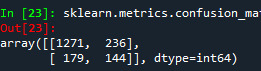
The diagonal values 1271 and 144 show the number of true negative and true positive classification. 170 shows the false negative and 236 show false positive.

We can also see the accuracy of the model which shows 0.77 which means 77% of sample has been classified correctly.

  The code used for building the model, training and testing and diplaying the tree is as follows: 

from pandas import Series, DataFrame

import pandas as pd

import numpy as np

import os

import matplotlib.pylab as plt

from sklearn.model_selection import train_test_split

from sklearn.tree import DecisionTreeClassifier

from sklearn.metrics import classification_report

import sklearn.metrics

 #Load the dataset

AH_data = pd.read_csv("tree_addhealth.csv")

data_clean = AH_data.dropna()

data_clean.dtypes

data_clean.describe()

 """

Modeling and Prediction

"""

#Split into training and testing sets

predictors = data_clean[['BIO_SEX','HISPANIC','WHITE','BLACK','NAMERICAN','ASIAN',

'age','ALCEVR1','ALCPROBS1','marever1','cocever1','inhever1','cigavail','DEP1',

'ESTEEM1','VIOL1','PASSIST','DEVIANT1','SCHCONN1','GPA1','EXPEL1','FAMCONCT','PARACTV',

'PARPRES']]

 targets = data_clean.TREG1

 pred_train, pred_test, tar_train, tar_test  =   train_test_split(predictors, targets, test_size=.4)

pred_train.shape

pred_test.shape

tar_train.shape

tar_test.shape

 #Build model on training data

classifier=DecisionTreeClassifier()

classifier=classifier.fit(pred_train,tar_train)

predictions=classifier.predict(pred_test)

sklearn.metrics.confusion_matrix(tar_test,predictions)

sklearn.metrics.accuracy_score(tar_test, predictions)

 #Displaying the decision tree

from sklearn import tree

#from StringIO import StringIO

from io import StringIO

#from StringIO import StringIO

from IPython.display import Image

out = StringIO()

 tree.export_graphviz(classifier, out_file=out)

tree.plot_tree(classifier,max_depth=2,fontsize=7)

The resulting tree start with a variable i.e. whether they use marijuana or no. fi the values is less than 0.5 then it splits to the left side which means there is no use of marijuana. Hence out of 2745, 2079 do not use marijuana and 666 do.

Among those individuals with no marijuana we can see how many consume alcohol (next variable) and how many don’t.

It seen than out of those people who do not take marijuana and do not consume alcohol,1169 are non-regular smokers and 46 are regular smokers. Out of people who don’t take in marijuana and consume alcohol we have 742 who are not regular and 122 are regular.  

On the right side of the tree, among individuals who have used marijuana and drank alcohol, 

220 are not regular smokers while 269 are. While among those individuals who have used marijuana but have not drank alcohol, 130 are not regular smokers, while 47 are.

  Gini index is use as splitting criteria. Now if we re run the model the values will slightly differ as python will randomly select 60% for training.