machinelearningcoursera

[machinelearningcoursera]

K-mean Analysis

Script:

from pandas import Series, DataFrame import pandas as pd import numpy as np import matplotlib.pylab as plt from sklearn.model_selection import train_test_split from sklearn import preprocessing from sklearn.cluster import KMeans import os """ Data Management """

data = pd.read_csv("tree_addhealth.csv")

upper-case all DataFrame column names

data.columns = map(str.upper, data.columns)

Data Management

data_clean = data.dropna()

subset clustering variables

cluster=data_clean[['ALCEVR1','MAREVER1','ALCPROBS1','DEVIANT1','VIOL1', 'DEP1','ESTEEM1','SCHCONN1','PARACTV', 'PARPRES','FAMCONCT']] cluster.describe()

standardize clustering variables to have mean=0 and sd=1

clustervar=cluster.copy() clustervar['ALCEVR1']=preprocessing.scale(clustervar['ALCEVR1'].astype('float64')) clustervar['ALCPROBS1']=preprocessing.scale(clustervar['ALCPROBS1'].astype('float64')) clustervar['MAREVER1']=preprocessing.scale(clustervar['MAREVER1'].astype('float64')) clustervar['DEP1']=preprocessing.scale(clustervar['DEP1'].astype('float64')) clustervar['ESTEEM1']=preprocessing.scale(clustervar['ESTEEM1'].astype('float64')) clustervar['VIOL1']=preprocessing.scale(clustervar['VIOL1'].astype('float64')) clustervar['DEVIANT1']=preprocessing.scale(clustervar['DEVIANT1'].astype('float64')) clustervar['FAMCONCT']=preprocessing.scale(clustervar['FAMCONCT'].astype('float64')) clustervar['SCHCONN1']=preprocessing.scale(clustervar['SCHCONN1'].astype('float64')) clustervar['PARACTV']=preprocessing.scale(clustervar['PARACTV'].astype('float64')) clustervar['PARPRES']=preprocessing.scale(clustervar['PARPRES'].astype('float64'))

split data into train and test sets

clus_train, clus_test = train_test_split(clustervar, test_size=.3, random_state=123)

k-means cluster analysis for 1-9 clusters

from scipy.spatial.distance import cdist clusters=range(1,9) meandist=[]

for k in clusters: model=KMeans(n_clusters=k) model.fit(clus_train) clusassign=model.predict(clus_train) meandist.append(sum(np.min(cdist(clus_train, model.cluster_centers_, 'euclidean'), axis=1)) / clus_train.shape[0])

""" Plot average distance from observations from the cluster centroid to use the Elbow Method to identify number of clusters to choose """

plt.plot(clusters, meandist) plt.xlabel('Number of clusters') plt.ylabel('Average distance') plt.title('Selecting k with the Elbow Method')

Interpret 3 cluster solution

model3=KMeans(n_clusters=2) model3.fit(clus_train) clusassign=model3.predict(clus_train)

plot clusters

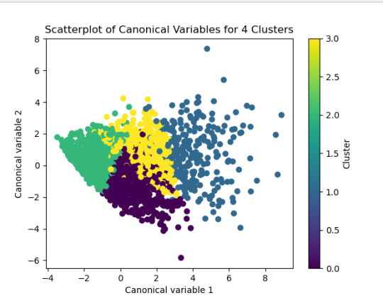
from sklearn.decomposition import PCA pca_2 = PCA(2) plot_columns = pca_2.fit_transform(clus_train) plt.scatter(x=plot_columns[:,0], y=plot_columns[:,1], c=model3.labels_) plt.xlabel('Canonical variable 1') plt.ylabel('Canonical variable 2') plt.title('Scatterplot of Canonical Variables for 4 Clusters')

Add the legend to the plot

import matplotlib.patches as mpatches patches = [mpatches.Patch(color=plt.cm.viridis(i/4), label=f'Cluster {i}') for i in range(4)]

plt.legend(handles=patches, title="Clusters") plt.show()

""" BEGIN multiple steps to merge cluster assignment with clustering variables to examine cluster variable means by cluster """

create a unique identifier variable from the index for the

cluster training data to merge with the cluster assignment variable

clus_train.reset_index(level=0, inplace=True)

create a list that has the new index variable

cluslist=list(clus_train['index'])

create a list of cluster assignments

labels=list(model3.labels_)

combine index variable list with cluster assignment list into a dictionary

newlist=dict(zip(cluslist, labels)) newlist

convert newlist dictionary to a dataframe

newclus=DataFrame.from_dict(newlist, orient='index') newclus

rename the cluster assignment column

newclus.columns = ['cluster']

now do the same for the cluster assignment variable

create a unique identifier variable from the index for the

cluster assignment dataframe

to merge with cluster training data

newclus.reset_index(level=0, inplace=True)

merge the cluster assignment dataframe with the cluster training variable dataframe

by the index variable

merged_train=pd.merge(clus_train, newclus, on='index') merged_train.head(n=100)

cluster frequencies

merged_train.cluster.value_counts()

""" END multiple steps to merge cluster assignment with clustering variables to examine cluster variable means by cluster """

FINALLY calculate clustering variable means by cluster

clustergrp = merged_train.groupby('cluster').mean() print ("Clustering variable means by cluster") print(clustergrp)

validate clusters in training data by examining cluster differences in GPA using ANOVA

first have to merge GPA with clustering variables and cluster assignment data

gpa_data=data_clean['GPA1']

split GPA data into train and test sets

gpa_train, gpa_test = train_test_split(gpa_data, test_size=.3, random_state=123) gpa_train1=pd.DataFrame(gpa_train) gpa_train1.reset_index(level=0, inplace=True) merged_train_all=pd.merge(gpa_train1, merged_train, on='index') sub1 = merged_train_all[['GPA1', 'cluster']].dropna()

import statsmodels.formula.api as smf import statsmodels.stats.multicomp as multi

gpamod = smf.ols(formula='GPA1 ~ C(cluster)', data=sub1).fit() print (gpamod.summary())

print ('means for GPA by cluster') m1= sub1.groupby('cluster').mean() print (m1)

print ('standard deviations for GPA by cluster') m2= sub1.groupby('cluster').std() print (m2)

mc1 = multi.MultiComparison(sub1['GPA1'], sub1['cluster']) res1 = mc1.tukeyhsd() print(res1.summary())

------------------------------------------------------------------------------

PLOTS:

------------------------------------------------------------------------------ANALYSING:

The K-mean cluster analysis is trying to identify subgroups of adolescents based on their similarity using the following 11 variables:

(Binary variables)

ALCEVR1 = ever used alcohol

MAREVER1 = ever used marijuana

(Quantitative variables)

ALCPROBS1 = Alcohol problem

DEVIANT1 = behaviors scale

VIOL1 = Violence scale

DEP1 = depression scale

ESTEEM1 = Self-esteem

SCHCONN1= School connectiveness

PARACTV = parent activities

PARPRES = parent presence

FAMCONCT = family connectiveness

The test was split with 70% for the training set and 30% for the test set. 9 clusters were conducted and the results are shown the plot 1. The plot suggest 2,4 , 5 and 6 solutions might be interpreted.

The second plot shows the canonical discriminant analyses of the 4 cluster solutions. Clusters 0 and 3 are very densely packed together with relatively low within-cluster variance whereas clusters 1 and 2 were spread out more than the other clusters, especially cluster 1 which means there is higher variance within the cluster. The number of clusters we would need to use is less the 3.

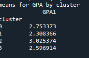
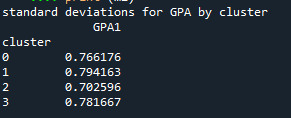
Students in cluster 2 had higher GPA values with an SD of 0.70 and cluster 1 had lower GPA values with an SD of 0.79

[machinelearningcoursera]

Lasso Regression

SCRIPT:

from pandas import Series, DataFrame import pandas as pd import numpy as np import os

from pandas import Series, DataFrame

import pandas as pd import numpy as np import matplotlib.pylab as plt from sklearn.model_selection import train_test_split from sklearn.linear_model import LassoLarsCV

Load the dataset

data = pd.read_csv("_358bd6a81b9045d95c894acf255c696a_nesarc_pds.csv") data=pd.DataFrame(data) data = data.replace(r'^\s*$', 101, regex=True)

upper-case all DataFrame column names

data.columns = map(str.upper, data.columns)

Data Management

data_clean = data.dropna()

select predictor variables and target variable as separate data sets

predvar= data_clean[['SEX','S1Q1E','S1Q7A9','S1Q7A10','S2AQ5A','S2AQ1','S2BQ1A20','S2CQ1','S2CQ2A10']]

target = data_clean.S2AQ5B

standardize predictors to have mean=0 and sd=1

predictors=predvar.copy() from sklearn import preprocessing predictors['SEX']=preprocessing.scale(predictors['SEX'].astype('float64')) predictors['S1Q1E']=preprocessing.scale(predictors['S1Q1E'].astype('float64')) predictors['S1Q7A9']=preprocessing.scale(predictors['S1Q7A9'].astype('float64')) predictors['S1Q7A10']=preprocessing.scale(predictors['S1Q7A10'].astype('float64')) predictors['S2AQ5A']=preprocessing.scale(predictors['S2AQ5A'].astype('float64')) predictors['S2AQ1']=preprocessing.scale(predictors['S2AQ1'].astype('float64')) predictors['S2BQ1A20']=preprocessing.scale(predictors['S2BQ1A20'].astype('float64')) predictors['S2CQ1']=preprocessing.scale(predictors['S2CQ1'].astype('float64')) predictors['S2CQ2A10']=preprocessing.scale(predictors['S2CQ2A10'].astype('float64'))

split data into train and test sets

pred_train, pred_test, tar_train, tar_test = train_test_split(predictors, target, test_size=.3, random_state=150)

specify the lasso regression model

model=LassoLarsCV(cv=10, precompute=False).fit(pred_train,tar_train)

print variable names and regression coefficients

dict(zip(predictors.columns, model.coef_))

plot coefficient progression

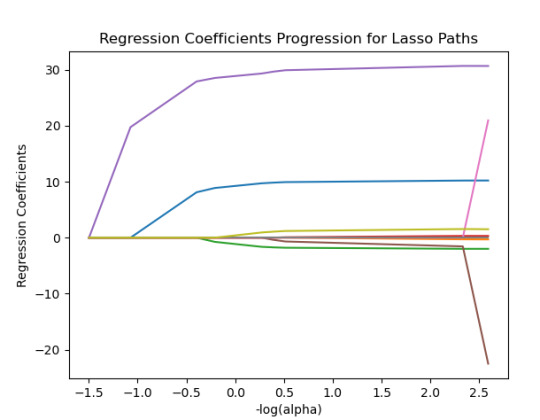
m_log_alphas = -np.log10(model.alphas_) ax = plt.gca() plt.plot(m_log_alphas, model.coef_path_.T) plt.axvline(-np.log10(model.alpha_), linestyle='--', color='k', label='alpha CV') plt.ylabel('Regression Coefficients') plt.xlabel('-log(alpha)') plt.title('Regression Coefficients Progression for Lasso Paths')

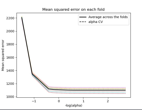
plot mean square error for each fold

m_log_alphascv = -np.log10(model.cv_alphas_) plt.figure() plt.plot(m_log_alphascv, model.mse_path_, ':') plt.plot(m_log_alphascv, model.mse_path_.mean(axis=-1), 'k', label='Average across the folds', linewidth=2) plt.axvline(-np.log10(model.alpha_), linestyle='--', color='k', label='alpha CV') plt.legend() plt.xlabel('-log(alpha)') plt.ylabel('Mean squared error') plt.title('Mean squared error on each fold')

MSE from training and test data

from sklearn.metrics import mean_squared_error train_error = mean_squared_error(tar_train, model.predict(pred_train)) test_error = mean_squared_error(tar_test, model.predict(pred_test)) print ('training data MSE') print(train_error) print ('test data MSE') print(test_error)

R-square from training and test data

rsquared_train=model.score(pred_train,tar_train) rsquared_test=model.score(pred_test,tar_test) print ('training data R-square') print(rsquared_train) print ('test data R-square') print(rsquared_test)

------------------------------------------------------------------------------

Graphs:

------------------------------------------------------------------------------

Analysing:

Output:

{'SEX': 10.217613940138108, 'S1Q1E': -0.31812083770240274, -ORIGIN OR DESCENT 'S1Q7A9': -1.9895640844032882, -PRESENT SITUATION INCLUDES RETIRED 'S1Q7A10': 0.30762235836398083, -PRESENT SITUATION INCLUDES IN SCHOOL FULL TIME 'S2AQ5A': 30.66524941440075, 'S2AQ1': -41.766164381325154, -DRANK AT LEAST 1 ALCOHOLIC DRINK IN LIFE 'S2BQ1A20': 73.94927622433774, - EVER HAVE JOB OR SCHOOL TROUBLES BECAUSE OF DRINKING 'S2CQ1': -33.74074926708572, -EVER SOUGHT HELP BECAUSE OF DRINKING 'S2CQ2A10': 1.6103002338271737} -EVER WENT TO EMPLOYEE ASSISTANCE PROGRAM (EAP)

training data MSE 1097.5883983117358 test data MSE 1098.0847471196266 training data R-square 0.50244242170729 test data R-square 0.4974333966086808

------------------------------------------------------------------------------

Conclusions:

I was looking at the questions, how often Brank beer in the last 12 Months?

We can see that the following variables are the most important variables to be able to answer the questions.

S2BQ1A20:EVER HAVE JOB OR SCHOOL TROUBLES BECAUSE OF DRINKING

S2AQ1:DRANK AT LEAST 1 ALCOHOLIC DRINK IN LIFE

S2CQ1:EVER SOUGHT HELP BECAUSE OF DRINKING

All the important variables are related to drinking. The Root squared for both the training and the test data is very small and very similar which means the training data set wasn't overfitted and not too biased.

30% was the training set and 70% was the test set, each set had 150 random states. The graph are showing 10 lasso regression coefficients

[machinelearningcoursera]

Random Forest

Script:

from pandas import Series, DataFrame import pandas as pd import numpy as np import os import matplotlib.pylab as plt from sklearn.model_selection import train_test_split from sklearn.tree import DecisionTreeClassifier from sklearn.metrics import classification_report import sklearn.metrics # Feature Importance from sklearn import datasets from sklearn.ensemble import ExtraTreesClassifier

current_directory = os.getcwd() """ Data Engineering and Analysis """

Load the dataset

AH_data = pd.read_csv("tree_addhealth.csv")

Replace empty cells (those containing None or blank strings) with NaN

data_clean = AH_data.dropna()

data_clean.dtypes data_clean.describe()

Split into training and testing sets

predictors = data_clean[['age','BLACK','WHITE','BIO_SEX','cocever1','VIOL1','GPA1']]

targets = data_clean.TREG1

pred_train, pred_test, tar_train, tar_test = train_test_split(predictors, targets, test_size=.4)

pred_train.shape pred_test.shape tar_train.shape tar_test.shape

Build model on training data

from sklearn.ensemble import RandomForestClassifier

classifier=RandomForestClassifier(n_estimators=25) classifier=classifier.fit(pred_train,tar_train)

predictions=classifier.predict(pred_test)

sklearn.metrics.confusion_matrix(tar_test,predictions) sklearn.metrics.accuracy_score(tar_test, predictions)

fit an Extra Trees model to the data

model = ExtraTreesClassifier() model.fit(pred_train,tar_train)

display the relative importance of each attribute

print(model.feature_importances_)

""" Running a different number of trees and see the effect of that on the accuracy of the prediction """

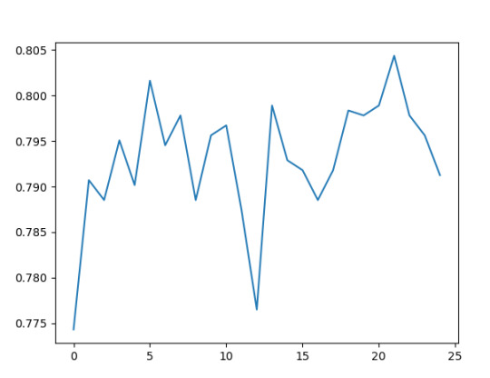
trees=range(25) accuracy=np.zeros(25)

for idx in range(len(trees)): classifier=RandomForestClassifier(n_estimators=idx + 1) classifier=classifier.fit(pred_train,tar_train) predictions=classifier.predict(pred_test) accuracy[idx]=sklearn.metrics.accuracy_score(tar_test, predictions)

plt.cla() plt.plot(trees, accuracy)

------------------------------------------------------------------------------

The data used:

Trying to answer the question, "Are you a regularly smocking?" based on the parameters I have used.

age

Black

White

Bio Sex

Every use cocaine

Violance behavior scale

Grades point average.

------------------------------------------------------------------------------Results

By running the random forest, I have an accuracy of 79% where 1361= True positive, 91=false negative, 114=True negative and 264= false positive.

Within the analyses, we can see that the age is the most important variable with 49% followed by the Grade point average with 23% and the violence scales with 16%.

The Race and Bio sex is not the most important factors which is what we are expecting.

------------------------------------------------------------------------------

Accuracy of each Tree: I have done 25 trees for this exercise.

[machinelearningcoursera]

Week one Classification Tree

SCRIPT

------------------------------------------------------------------------------

"""Imports"""

import matplotlib.pylab as plt from sklearn.model_selection import train_test_split

from sklearn.cross_validation import train_test_split

from sklearn.tree import DecisionTreeClassifier from sklearn.metrics import classification_report import sklearn.metrics

"""Opening the file and cleaning the data"""

os.chdir("/M/machine learning")

AH_data = pd.read_csv("tree_addhealth.csv")

data_clean = AH_data.dropna()

data_clean.dtypes data_clean.describe()

"""Select my predictors and target values"""

predictors = data_clean[[ 'age','ALCEVR1', 'PASSIST','GPA1' ]]

targets = data_clean.TREG1

"""Split the data into training (60%) and testing (40%) set"""

pred_train, pred_test, tar_train, tar_test = train_test_split(predictors, targets, test_size=.4)

"""Run the training data with the decision tree"""

classifier=DecisionTreeClassifier() classifier=classifier.fit(pred_train,tar_train)

"""Run the predictions, check the matric and accuracy"""

predictions=classifier.predict(pred_test)

sklearn.metrics.confusion_matrix(tar_test,predictions)

sklearn.metrics.accuracy_score(tar_test, predictions)

"""Create the display of the image"""

Displaying the decision tree

from sklearn import tree

from StringIO import StringIO

from io import StringIO

from StringIO import StringIO

from IPython.display import Image out = StringIO() tree.export_graphviz(classifier, out_file=out)

import pydotplus graph=pydotplus.graph_from_dot_data(out.getvalue())

Image(graph.create_png())

------------------------------------------------------------------------------

Output

[[1341, 163], [ 252, 74]]

1341 are true positive smokers, 74 are false negative smokers, 163 are true negative smokers, and 252 are negative positive smokers.

With the accuracy of 77%

Explanatory variable used- Quantative

Age

GPA1

Explanatory variable used-categorical

Ever drank alcohol

Parent on public assistance

All different variables which are not linked to each other to check the accuracy of the model.