manju098 - Tumblr blog

manju098 · 2 years ago

Text

Running a k-means Cluster Analysis:

Machine Learning for Data Analysis

Week 4: Running a k-means Cluster Analysis

A k-means cluster analysis was conducted to identify underlying subgroups of countries based on their similarity of responses on 7 variables that represent characteristics that could have an impact on internet use rates. Clustering variables included quantitative variables measuring income per person, employment rate, female employment rate, polity score, alcohol consumption, life expectancy, and urban rate. All clustering variables were standardized to have a mean of 0 and a standard deviation of 1.

Because the GapMinder dataset which I am using is relatively small (N < 250), I have not split the data into test and training sets. A series of k-means cluster analyses were conducted on the training data specifying k=1-9 clusters, using Euclidean distance. The variance in the clustering variables that was accounted for by the clusters (r-square) was plotted for each of the nine cluster solutions in an elbow curve to provide guidance for choosing the number of clusters to interpret.

Load the data, set the variables to numeric, and clean the data of NA values

In [1]:''' Code for Peer-graded Assignments: Running a k-means Cluster Analysis Course: Data Management and Visualization Specialization: Data Analysis and Interpretation ''' import pandas as pd import numpy as np import matplotlib.pyplot as plt import statsmodels.formula.api as smf import statsmodels.stats.multicomp as multi from sklearn.cross_validation import train_test_split from sklearn import preprocessing from sklearn.cluster import KMeans data = pd.read_csv('c:/users/greg/desktop/gapminder.csv', low_memory=False) data['internetuserate'] = pd.to_numeric(data['internetuserate'], errors='coerce') data['incomeperperson'] = pd.to_numeric(data['incomeperperson'], errors='coerce') data['employrate'] = pd.to_numeric(data['employrate'], errors='coerce') data['femaleemployrate'] = pd.to_numeric(data['femaleemployrate'], errors='coerce') data['polityscore'] = pd.to_numeric(data['polityscore'], errors='coerce') data['alcconsumption'] = pd.to_numeric(data['alcconsumption'], errors='coerce') data['lifeexpectancy'] = pd.to_numeric(data['lifeexpectancy'], errors='coerce') data['urbanrate'] = pd.to_numeric(data['urbanrate'], errors='coerce') sub1 = data.copy() data_clean = sub1.dropna()

Subset the clustering variables

In [2]:cluster = data_clean[['incomeperperson','employrate','femaleemployrate','polityscore', 'alcconsumption', 'lifeexpectancy', 'urbanrate']] cluster.describe()

Out[2]:incomeperpersonemployratefemaleemployratepolityscorealcconsumptionlifeexpectancyurbanratecount150.000000150.000000150.000000150.000000150.000000150.000000150.000000mean6790.69585859.26133348.1006673.8933336.82173368.98198755.073200std9861.86832710.38046514.7809996.2489165.1219119.90879622.558074min103.77585734.90000212.400000-10.0000000.05000048.13200010.40000025%592.26959252.19999939.599998-1.7500002.56250062.46750036.41500050%2231.33485558.90000248.5499997.0000006.00000072.55850057.23000075%7222.63772165.00000055.7250009.00000010.05750076.06975071.565000max39972.35276883.19999783.30000310.00000023.01000083.394000100.000000

Standardize the clustering variables to have mean = 0 and standard deviation = 1

In [3]:clustervar=cluster.copy() clustervar['incomeperperson']=preprocessing.scale(clustervar['incomeperperson'].astype('float64')) clustervar['employrate']=preprocessing.scale(clustervar['employrate'].astype('float64')) clustervar['femaleemployrate']=preprocessing.scale(clustervar['femaleemployrate'].astype('float64')) clustervar['polityscore']=preprocessing.scale(clustervar['polityscore'].astype('float64')) clustervar['alcconsumption']=preprocessing.scale(clustervar['alcconsumption'].astype('float64')) clustervar['lifeexpectancy']=preprocessing.scale(clustervar['lifeexpectancy'].astype('float64')) clustervar['urbanrate']=preprocessing.scale(clustervar['urbanrate'].astype('float64'))

Split the data into train and test sets

In [4]:clus_train, clus_test = train_test_split(clustervar, test_size=.3, random_state=123)

Perform k-means cluster analysis for 1-9 clusters

In [5]:from scipy.spatial.distance import cdist clusters = range(1,10) meandist = [] for k in clusters: model = KMeans(n_clusters = k) model.fit(clus_train) clusassign = model.predict(clus_train) meandist.append(sum(np.min(cdist(clus_train, model.cluster_centers_, 'euclidean'), axis=1)) / clus_train.shape[0])

Plot average distance from observations from the cluster centroid to use the Elbow Method to identify number of clusters to choose

In [6]:plt.plot(clusters, meandist) plt.xlabel('Number of clusters') plt.ylabel('Average distance') plt.title('Selecting k with the Elbow Method') plt.show()

In [7]:model3 = KMeans(n_clusters=4) model3.fit(clus_train) clusassign = model3.predict(clus_train)

Plot the clusters

In [8]:from sklearn.decomposition import PCA pca_2 = PCA(2) plt.figure() plot_columns = pca_2.fit_transform(clus_train) plt.scatter(x=plot_columns[:,0], y=plot_columns[:,1], c=model3.labels_,) plt.xlabel('Canonical variable 1') plt.ylabel('Canonical variable 2') plt.title('Scatterplot of Canonical Variables for 4 Clusters') plt.show()

Begin multiple steps to merge cluster assignment with clustering variables to examine cluster variable means by cluster.

Create a unique identifier variable from the index for the cluster training data to merge with the cluster assignment variable.

In [9]:clus_train.reset_index(level=0, inplace=True)

Create a list that has the new index variable

In [10]:cluslist = list(clus_train['index'])

Create a list of cluster assignments

In [11]:labels = list(model3.labels_)

Combine index variable list with cluster assignment list into a dictionary

In [12]:newlist = dict(zip(cluslist, labels)) print (newlist) {2: 1, 4: 2, 6: 0, 10: 0, 11: 3, 14: 2, 16: 3, 17: 0, 19: 2, 22: 2, 24: 3, 27: 3, 28: 2, 29: 2, 31: 2, 32: 0, 35: 2, 37: 3, 38: 2, 39: 3, 42: 2, 45: 2, 47: 1, 53: 3, 54: 3, 55: 1, 56: 3, 58: 2, 59: 3, 63: 0, 64: 0, 66: 3, 67: 2, 68: 3, 69: 0, 70: 2, 72: 3, 77: 3, 78: 2, 79: 2, 80: 3, 84: 3, 88: 1, 89: 1, 90: 0, 91: 0, 92: 0, 93: 3, 94: 0, 95: 1, 97: 2, 100: 0, 102: 2, 103: 2, 104: 3, 105: 1, 106: 2, 107: 2, 108: 1, 113: 3, 114: 2, 115: 2, 116: 3, 123: 3, 126: 3, 128: 3, 131: 2, 133: 3, 135: 2, 136: 0, 139: 0, 140: 3, 141: 2, 142: 3, 144: 0, 145: 1, 148: 3, 149: 2, 150: 3, 151: 3, 152: 3, 153: 3, 154: 3, 158: 3, 159: 3, 160: 2, 173: 0, 175: 3, 178: 3, 179: 0, 180: 3, 183: 2, 184: 0, 186: 1, 188: 2, 194: 3, 196: 1, 197: 2, 200: 3, 201: 1, 205: 2, 208: 2, 210: 1, 211: 2, 212: 2}

Convert newlist dictionary to a dataframe

In [13]:newclus = pd.DataFrame.from_dict(newlist, orient='index') newclus

Out[13]:0214260100113142163170192222243273282292312320352373382393422452471533543551563582593630......145114831492150315131523153315431583159316021730175317831790180318321840186118821943196119722003201120522082210121122122

105 rows × 1 columns

Rename the cluster assignment column

In [14]:newclus.columns = ['cluster']

Repeat previous steps for the cluster assignment variable

Create a unique identifier variable from the index for the cluster assignment dataframe to merge with cluster training data

In [15]:newclus.reset_index(level=0, inplace=True)

Merge the cluster assignment dataframe with the cluster training variable dataframe by the index variable

In [16]:merged_train = pd.merge(clus_train, newclus, on='index') merged_train.head(n=100)

Out[16]:indexincomeperpersonemployratefemaleemployratepolityscorealcconsumptionlifeexpectancyurbanratecluster0159-0.393486-0.0445910.3868770.0171271.843020-0.0160990.79024131196-0.146720-1.591112-1.7785290.498818-0.7447360.5059900.6052111270-0.6543650.5643511.0860520.659382-0.727105-0.481382-0.2247592329-0.6791572.3138522.3893690.3382550.554040-1.880471-1.9869992453-0.278924-0.634202-0.5159410.659382-0.1061220.4469570.62033335153-0.021869-1.020832-0.4073320.9805101.4904110.7233920.2778493635-0.6665191.1636281.004595-0.785693-0.715352-2.084304-0.7335932714-0.6341100.8543230.3733010.177691-1.303033-0.003846-1.24242828116-0.1633940.119726-0.3394510.338255-1.1659070.5304950.67993439126-0.630263-1.446126-0.3055100.6593823.1711790.033923-0.592152310123-0.163655-0.460219-0.8010420.980510-0.6448300.444628-0.560127311106-0.640452-0.2862350.1153530.659382-0.247166-2.104758-1.317152212142-0.635480-0.808186-0.7874660.0171271.155433-1.731823-0.29859331389-0.615980-2.113062-2.423400-0.625129-1.2442650.0060770.512695114160-0.6564731.9852172.199302-1.1068200.620643-1.371039-1.63383921556-0.430694-0.102586-0.2240530.659382-0.5547190.3254460.250272316180-0.559059-0.402224-0.6041870.338255-1.1776610.603401-1.777949317133-0.419521-1.668438-0.7331610.3382551.032020-0.659900-0.81098631831-0.618282-0.0155940.061048-1.2673840.211226-1.7590620.075026219171.801349-1.030498-0.4344840.6593820.7029191.1165791.8808550201450.447771-0.827517-1.731013-1.909640-1.1561120.4042250.7359771211000.974856-0.034925-0.0068330.6593822.4150301.1806761.173646022178-0.309804-1.755430-0.9368040.8199460.653945-1.6388680.2520513231732.6193200.3033760.217174-0.946256-1.0346581.2296851.99827802459-0.056177-0.2669040.2714790.8199462.0408730.5916550.63990432568-0.562821-0.3538960.0271070.338255-0.0316830.481486-0.1037773261080.111383-1.030498-1.690284-1.749076-1.3167450.5879080.999290127212-0.6582520.7286690.678765-0.464565-0.364702-1.781946-0.78874722819-0.6525281.1926250.6855540.498818-0.928876-1.306335-0.617060229188-0.662484-0.4505530.135717-1.106820-0.672255-0.147127-1.2726732..............................70140-0.594402-0.044591-0.8214060.819946-0.3157280.5125720.074137371148-0.0905570.052066-0.3190860.8199460.0936890.7235950.80625437211-0.4523170.1583900.549792-1.7490761.2768870.177913-0.140250373641.636776-0.779188-0.1697480.8199461.1084191.2715050.99128407484-0.117682-1.156153-0.5295180.9805101.8214720.5500380.5527263751750.604211-0.3248980.0882000.9805101.5903171.048938-0.287918376197-0.481087-0.0735890.393665-2.070203-0.356866-0.404628-0.287029277183-0.506714-0.808186-0.067926-2.070203-0.347071-2.051902-1.340281278210-0.628790-1.958410-1.887139-0.946256-1.297156-0.353290-1.08675317954-0.5150780.042400-0.1765360.1776910.5109430.6733710.467327380114-0.6661982.2945212.111056-0.625129-1.077755-0.229248-1.1365692814-0.5503841.5889211.445822-0.946256-0.245207-1.8114130.072358282911.575455-0.769523-0.1154430.980510-0.8426821.2795041.62732708377-0.5015740.332373-0.2783580.6593820.0545110.221758-0.28880838466-0.265535-0.0252600.305419-0.1434370.516820-0.6358011.332879385921.240375-1.243145-0.8349830.9805100.5677521.3035020.5785230862011.4545511.540592-0.733161-1.909640-1.2344700.7659211.014413187105-0.004485-1.281808-1.7513770.498818-0.8857790.3704051.418278188205-0.593947-0.1702460.305419-2.070203-0.629158-0.070373-0.8118762891540.504036-0.1605810.1696570.9805101.3846291.0649370.19511839045-0.6307520.061732-0.678856-0.625129-0.068902-1.377621-0.27991229197-0.6432031.3472771.2557550.498818-0.576267-1.199710-1.488839292632.067368-0.1992430.3597250.9805101.2298731.1133390.365916093211-0.6469130.1680550.3665130.498818-0.638953-2.020815-0.874146294158-0.422620-0.943506-0.2919340.8199461.8273490.505990-0.037060395135-0.6635950.2453810.4411820.338255-0.862272-0.018934-1.68276529679-0.6744750.6416770.1221410.338255-0.572349-2.111239-1.1223362971790.882197-0.653534-0.4344840.9805100.9810881.2578350.980609098149-0.6151691.0766361.4118810.017127-0.623282-0.626890-1.891814299113-0.464904-2.354706-1.4459120.8199460.4149550.5938830.5260393

100 rows × 9 columns

Cluster frequencies

In [17]:merged_train.cluster.value_counts()

Out[17]:3 39 2 35 0 18 1 13 Name: cluster, dtype: int64

Calculate clustering variable means by cluster

In [18]:clustergrp = merged_train.groupby('cluster').mean() print ("Clustering variable means by cluster") clustergrp Clustering variable means by cluster

Out[18]:indexincomeperpersonemployratefemaleemployratepolityscorealcconsumptionlifeexpectancyurbanratecluster093.5000001.846611-0.1960210.1010220.8110260.6785411.1956961.0784621117.461538-0.154556-1.117490-1.645378-1.069767-1.0827280.4395570.5086582100.657143-0.6282270.8551520.873487-0.583841-0.506473-1.034933-0.8963853107.512821-0.284648-0.424778-0.2000330.5317550.6146160.2302010.164805

Validate clusters in training data by examining cluster differences in internetuserate using ANOVA. First, merge internetuserate with clustering variables and cluster assignment data

In [19]:internetuserate_data = data_clean['internetuserate']

Split internetuserate data into train and test sets

In [20]:internetuserate_train, internetuserate_test = train_test_split(internetuserate_data, test_size=.3, random_state=123) internetuserate_train1=pd.DataFrame(internetuserate_train) internetuserate_train1.reset_index(level=0, inplace=True) merged_train_all=pd.merge(internetuserate_train1, merged_train, on='index') sub5 = merged_train_all[['internetuserate', 'cluster']].dropna()

In [21]:internetuserate_mod = smf.ols(formula='internetuserate ~ C(cluster)', data=sub5).fit() internetuserate_mod.summary()

Out[21]:

OLS Regression ResultsDep. Variable:internetuserateR-squared:0.679Model:OLSAdj. R-squared:0.669Method:Least SquaresF-statistic:71.17Date:Thu, 12 Jan 2017Prob (F-statistic):8.18e-25Time:20:59:17Log-Likelihood:-436.84No. Observations:105AIC:881.7Df Residuals:101BIC:892.3Df Model:3Covariance Type:nonrobustcoefstd errtP>|t|[95.0% Conf. Int.]Intercept75.20683.72720.1770.00067.813 82.601C(cluster)[T.1]-46.95175.756-8.1570.000-58.370 -35.534C(cluster)[T.2]-66.56684.587-14.5130.000-75.666 -57.468C(cluster)[T.3]-39.48604.506-8.7630.000-48.425 -30.547Omnibus:5.290Durbin-Watson:1.727Prob(Omnibus):0.071Jarque-Bera (JB):4.908Skew:0.387Prob(JB):0.0859Kurtosis:3.722Cond. No.5.90

Means for internetuserate by cluster

In [22]:m1= sub5.groupby('cluster').mean() m1

Out[22]:internetuseratecluster075.206753128.25501828.639961335.720760

Standard deviations for internetuserate by cluster

In [23]:m2= sub5.groupby('cluster').std() m2

Out[23]:internetuseratecluster014.093018121.75775228.399554319.057835

In [24]:mc1 = multi.MultiComparison(sub5['internetuserate'], sub5['cluster']) res1 = mc1.tukeyhsd() res1.summary()

Out[24]:

Multiple Comparison of Means - Tukey HSD,FWER=0.05group1group2meandifflowerupperreject01-46.9517-61.9887-31.9148True02-66.5668-78.5495-54.5841True03-39.486-51.2581-27.7139True12-19.6151-33.0335-6.1966True137.4657-5.76520.6965False2327.080817.461736.6999True

The elbow curve was inconclusive, suggesting that the 2, 4, 6, and 8-cluster solutions might be interpreted. The results above are for an interpretation of the 4-cluster solution.

In order to externally validate the clusters, an Analysis of Variance (ANOVA) was conducting to test for significant differences between the clusters on internet use rate. A tukey test was used for post hoc comparisons between the clusters. Results indicated significant differences between the clusters on internet use rate (F=71.17, p<.0001). The tukey post hoc comparisons showed significant differences between clusters on internet use rate, with the exception that clusters 0 and 2 were not significantly different from each other. Countries in cluster 1 had the highest internet use rate (mean=75.2, sd=14.1), and cluster 3 had the lowest internet use rate (mean=8.64, sd=8.40).

0 notes

manju098 · 2 years ago

Text

Running a Lasso Regression Analysis

import pandas as pd import numpy as np import matplotlib.pylab as plt from sklearn.cross_validation import train_test_split from sklearn.linear_model import LassoLarsCV

Load the dataset

data = pd.read_csv("gapminder_ghana_updated.csv")

DATA MANAGEMENT

CONVERTING SOME QUANTITATIVE VARIABLES INTO CATEGORICAL VARIABLES TO GET FEEL

OF LASSO REGRESSION

data_clean = data.dropna()

check minimum and maximum values of totalpopulationfemale and create categorical

variable out of it

print(data_clean["totalpopulationfemale"].describe())

def totalpopulationfemaleGrp(row): if row["totalpopulationfemale"]<=7758806: return 0 elif row["totalpopulationfemale"] > 7758806: return 1

data_clean["totalpopulationfemaleGrp"] = data_clean.apply(lambda row:totalpopulationfemaleGrp(row), axis =1 )

check values in totalpopulationfemaleGrp

checktotFemPop = data_clean["totalpopulationfemaleGrp"].value_counts(sort=False, dropna=True) print(checktotFemPop)

check minimum and maximum values of malebloodpressure and create categorical

variable out of it

print(data_clean["malebloodpressure"].describe())

def malebloodpressureGrp(row): if row["malebloodpressure"]<=129: return 0 elif row["malebloodpressure"] > 129: return 1

data_clean["malebloodpressureGrp"] = data_clean.apply(lambda row:totalpopulationfemaleGrp(row), axis =1 )

check values ink totalpopulationfemaleGrp

checkmaleblood = data_clean["malebloodpressureGrp"].value_counts(sort=False, dropna=True) print(checkmaleblood)

creating categorical explanatory variables out of exports

def exportsCatGrp (row): if row["exports"] <=40: return 0 elif row["exports"] >40: return 1

data_clean["exportsCatGrp"] = data_clean.apply(lambda row:exportsCatGrp(row), axis =1)

creating a categorical explanatry variable out of incomeperperson

def incomeLevelGrp (row): if row["incomeperperson"] <=2200: return 0 elif row["incomeperperson"] >2200: return 1

data_clean["incomeLevelGrp"] = data_clean.apply(lambda row:incomeLevelGrp(row), axis =1)

END OF DATA MANAGEMENT

predvar= data_clean[['incomeLevelGrp','exportsCatGrp','malebloodpressureGrp', 'totalpopulationfemaleGrp','inflation','agriculture','democracyscore', 'agriculturalland','aidreceived','aidreceivedperperson','realgdppercapita', 'femalebloodpressure','malebodymassindex','femalebodymassindex','underfivemortality', 'totalfertilityrate','cholesterolinmen','cholesterolinwomen','crudebirthrate', 'deadkidsperwoman','externaldebtstocks','energyuse']]

target = data_clean.lifeexpectancy

standardize predictors to have mean=0 and sd=1

predictors=predvar.copy() from sklearn import preprocessing predictors['incomeLevelGrp']=preprocessing.scale(predictors['incomeLevelGrp'].astype('float64')) predictors['exportsCatGrp']=preprocessing.scale(predictors['exportsCatGrp'].astype('float64')) predictors['inflation']=preprocessing.scale(predictors['inflation'].astype('float64')) predictors['agriculture']=preprocessing.scale(predictors['agriculture'].astype('float64')) predictors['democracyscore']=preprocessing.scale(predictors['democracyscore'].astype('float64')) predictors['agriculturalland']=preprocessing.scale(predictors['agriculturalland'].astype('float64')) predictors['aidreceived']=preprocessing.scale(predictors['aidreceived'].astype('float64')) predictors['aidreceivedperperson']=preprocessing.scale(predictors['aidreceivedperperson'].astype('float64')) predictors['realgdppercapita']=preprocessing.scale(predictors['realgdppercapita'].astype('float64')) predictors['malebloodpressureGrp']=preprocessing.scale(predictors['malebloodpressureGrp'].astype('float64')) predictors['femalebloodpressure']=preprocessing.scale(predictors['femalebloodpressure'].astype('float64')) predictors['malebodymassindex']=preprocessing.scale(predictors['malebodymassindex'].astype('float64')) predictors['femalebodymassindex']=preprocessing.scale(predictors['femalebodymassindex'].astype('float64')) predictors['underfivemortality']=preprocessing.scale(predictors['underfivemortality'].astype('float64')) predictors['totalfertilityrate']=preprocessing.scale(predictors['totalfertilityrate'].astype('float64')) predictors['cholesterolinmen']=preprocessing.scale(predictors['cholesterolinmen'].astype('float64')) predictors['cholesterolinwomen']=preprocessing.scale(predictors['cholesterolinwomen'].astype('float64')) predictors['crudebirthrate']=preprocessing.scale(predictors['crudebirthrate'].astype('float64')) predictors['deadkidsperwoman']=preprocessing.scale(predictors['deadkidsperwoman'].astype('float64')) predictors['externaldebtstocks']=preprocessing.scale(predictors['externaldebtstocks'].astype('float64')) predictors['energyuse']=preprocessing.scale(predictors['energyuse'].astype('float64')) predictors['totalpopulationfemaleGrp']=preprocessing.scale(predictors['totalpopulationfemaleGrp'].astype('float64'))

split data into train and test sets

pred_train, pred_test, tar_train, tar_test = train_test_split(predictors, target, test_size=.3, random_state=123)

specify the lasso regression model

model=LassoLarsCV(cv=10, precompute=False).fit(pred_train,tar_train)

print variable names and regression coefficients

dict(zip(predictors.columns, model.coef_))

plot coefficient progression

m_log_alphas = -np.log10(model.alphas_) ax = plt.gca() plt.plot(m_log_alphas, model.coef_path_.T) plt.axvline(-np.log10(model.alpha_), linestyle='--', color='k', label='alpha CV') plt.ylabel('Regression Coefficients') plt.xlabel('-log(alpha)') plt.title('Regression Coefficients Progression for Lasso Paths')

plot mean square error for each fold

m_log_alphascv = -np.log10(model.cv_alphas_) plt.figure() plt.plot(m_log_alphascv, model.cv_mse_path_, ':') plt.plot(m_log_alphascv, model.cv_mse_path_.mean(axis=-1), 'k', label='Average across the folds', linewidth=2) plt.axvline(-np.log10(model.alpha_), linestyle='--', color='k', label='alpha CV') plt.legend() plt.xlabel('-log(alpha)') plt.ylabel('Mean squared error') plt.title('Mean squared error on each fold')

MSE from training and test data

from sklearn.metrics import mean_squared_error train_error = mean_squared_error(tar_train, model.predict(pred_train)) test_error = mean_squared_error(tar_test, model.predict(pred_test)) print ('training data MSE') print(train_error) print ('test data MSE') print(test_error)

R-square from training and test data

rsquared_train=model.score(pred_train,tar_train) rsquared_test=model.score(pred_test,tar_test) print ('training data R-square') print(rsquared_train) print ('test data R-square') print(rsquared_test)

0 notes

manju098 · 2 years ago

Text

Running a Random Forest

import pandas as pd import numpy as np import matplotlib.pylab as plt from sklearn.model_selection import train_test_split, cross_val_score from sklearn.ensemble import RandomForestClassifier, ExtraTreesClassifier from sklearn.manifold import MDS from sklearn.metrics.pairwise import pairwise_distances from sklearn.metrics import accuracy_score import seaborn as sns %matplotlib inline

rnd_state = 4536 data = pd.read_csv('Data\winequality-red.csv', sep=';') data.info()

RangeIndex: 1599 entries, 0 to 1598 Data columns (total 12 columns): fixed acidity 1599 non-null float64 volatile acidity 1599 non-null float64 citric acid 1599 non-null float64 residual sugar 1599 non-null float64 chlorides 1599 non-null float64 free sulfur dioxide 1599 non-null float64 total sulfur dioxide 1599 non-null float64 density 1599 non-null float64 pH 1599 non-null float64 sulphates 1599 non-null float64 alcohol 1599 non-null float64 quality 1599 non-null int64 dtypes: float64(11), int64(1) memory usage: 150.0 KB data.head() fixed acidity volatile acidity citric acid residual sugar chlorides free sulfur dioxide total sulfur dioxide density pH sulphates alcohol quality 0 7.4 0.70 0.00 1.9 0.076 11.0 34.0 0.9978 3.51 0.56 9.4 5 1 7.8 0.88 0.00 2.6 0.098 25.0 67.0 0.9968 3.20 0.68 9.8 5 2 7.8 0.76 0.04 2.3 0.092 15.0 54.0 0.9970 3.26 0.65 9.8 5 3 11.2 0.28 0.56 1.9 0.075 17.0 60.0 0.9980 3.16 0.58 9.8 6 4 7.4 0.70 0.00 1.9 0.076 11.0 34.0 0.9978 3.51 0.56 9.4 5 data.describe() fixed acidity volatile acidity citric acid residual sugar chlorides free sulfur dioxide total sulfur dioxide density pH sulphates alcohol quality count 1599.000000 1599.000000 1599.000000 1599.000000 1599.000000 1599.000000 1599.000000 1599.000000 1599.000000 1599.000000 1599.000000 1599.000000 mean 8.319637 0.527821 0.270976 2.538806 0.087467 15.874922 46.467792 0.996747 3.311113 0.658149 10.422983 5.636023 std 1.741096 0.179060 0.194801 1.409928 0.047065 10.460157 32.895324 0.001887 0.154386 0.169507 1.065668 0.807569 min 4.600000 0.120000 0.000000 0.900000 0.012000 1.000000 6.000000 0.990070 2.740000 0.330000 8.400000 3.000000 25% 7.100000 0.390000 0.090000 1.900000 0.070000 7.000000 22.000000 0.995600 3.210000 0.550000 9.500000 5.000000 50% 7.900000 0.520000 0.260000 2.200000 0.079000 14.000000 38.000000 0.996750 3.310000 0.620000 10.200000 6.000000 75% 9.200000 0.640000 0.420000 2.600000 0.090000 21.000000 62.000000 0.997835 3.400000 0.730000 11.100000 6.000000 max 15.900000 1.580000 1.000000 15.500000 0.611000 72.000000 289.000000 1.003690 4.010000 2.000000 14.900000 8.000000 For visualization purposes, the number of dimensions was reduced to two by applying MDS method with cosine distance. The plot illustrates that our classes are not clearly divided into parts.

model = MDS(random_state=rnd_state, n_components=2, dissimilarity='precomputed') %time representation = model.fit_transform(pairwise_distances(data.iloc[:, :11], metric='cosine')) Wall time: 38.7 s colors = ["#9b59b6", "#3498db", "#95a5a6", "#e74c3c", "#34495e", "#2ecc71"] plt.figure(figsize=(12, 4))

plt.subplot(121) plt.scatter(representation[:, 0], representation[:, 1], c=colors)

plt.subplot(122) sns.countplot(x='quality', data=data, palette=sns.color_palette(colors));

predictors = data.iloc[:, :11] target = data.quality

In [8]:(predictors_train, predictors_test, target_train, target_test) = train_test_split(predictors, target, test_size = .3, random_state = rnd_state)

RandomForest classifier

In [9]:list_estimators = list(range(1, 50, 5)) rf_scoring = [] for n_estimators in list_estimators: classifier = RandomForestClassifier(random_state = rnd_state, n_jobs =-1, class_weight='balanced', n_estimators=n_estimators) score = cross_val_score(classifier, predictors_train, target_train, cv=5, n_jobs=-1, scoring = 'accuracy') rf_scoring.append(score.mean())

In [10]:plt.plot(list_estimators, rf_scoring) plt.title('Accuracy VS trees number');

predictors = data.iloc[:, :11] target = data.quality

In [8]:(predictors_train, predictors_test, target_train, target_test) = train_test_split(predictors, target, test_size = .3, random_state = rnd_state)

RandomForest classifier

In [10]:plt.plot(list_estimators, rf_scoring) plt.title('Accuracy VS trees number');

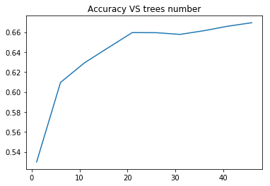
classifier = RandomForestClassifier(random_state = rnd_state, n_jobs =-1, class_weight='balanced', n_estimators=20) classifier.fit(predictors_train, target_train)

Out[11]:RandomForestClassifier(bootstrap=True, class_weight='balanced', criterion='gini', max_depth=None, max_features='auto', max_leaf_nodes=None, min_impurity_decrease=0.0, min_impurity_split=None, min_samples_leaf=1, min_samples_split=2, min_weight_fraction_leaf=0.0, n_estimators=20, n_jobs=-1, oob_score=False, random_state=4536, verbose=0, warm_start=False)

In [12]:prediction = classifier.predict(predictors_test)

In [13]:print('Confusion matrix:\n', pd.crosstab(target_test, prediction, colnames=['Predicted'], rownames=['Actual'], margins=True)) print('\nAccuracy: ', accuracy_score(target_test, prediction)) Confusion matrix: Predicted 3 4 5 6 7 All Actual 3 0 0 3 0 0 3 4 0 1 9 6 0 16 5 2 1 166 41 3 213 6 0 0 46 131 14 191 7 0 0 5 25 23 53 8 0 0 0 3 1 4 All 2 2 229 206 41 480 Accuracy: 0.66875

In [14]:feature_importance = pd.Series(classifier.feature_importances_, index=data.columns.values[:11]).sort_values(ascending=False) feature_importance

volatile acidity 0.133023 alcohol 0.130114 sulphates 0.129498 citric acid 0.106427 total sulfur dioxide 0.094647 chlorides 0.086298 density 0.079843 pH 0.066566 residual sugar 0.061344 fixed acidity 0.058251 free sulfur dioxide 0.053990 dtype: float64

In [15]:et_scoring = [] for n_estimators in list_estimators: classifier = ExtraTreesClassifier(random_state = rnd_state, n_jobs =-1, class_weight='balanced', n_estimators=n_estimators) score = cross_val_score(classifier, predictors_train, target_train, cv=5, n_jobs=-1, scoring = 'accuracy') et_scoring.append(score.mean())

In [16]:plt.plot(list_estimators, et_scoring) plt.title('Accuracy VS trees number');

classifier = ExtraTreesClassifier(random_state = rnd_state, n_jobs =-1, class_weight='balanced', n_estimators=12) classifier.fit(predictors_train, target_train)

Out[17]:ExtraTreesClassifier(bootstrap=False, class_weight='balanced', criterion='gini', max_depth=None, max_features='auto', max_leaf_nodes=None, min_impurity_decrease=0.0, min_impurity_split=None, min_samples_leaf=1, min_samples_split=2, min_weight_fraction_leaf=0.0, n_estimators=12, n_jobs=-1, oob_score=False, random_state=4536, verbose=0, warm_start=False)

In [18]:prediction = classifier.predict(predictors_test)

In [19]:print('Confusion matrix:\n', pd.crosstab(target_test, prediction, colnames=['Predicted'], rownames=['Actual'], margins=True)) print('\nAccuracy: ', accuracy_score(target_test, prediction)) Confusion matrix: Predicted 3 4 5 6 7 8 All Actual 3 0 1 2 0 0 0 3 4 0 0 9 7 0 0 16 5 2 2 168 39 2 0 213 6 0 0 49 130 11 1 191 7 0 0 2 27 24 0 53 8 0 0 0 3 1 0 4 All 2 3 230 206 38 1 480 Accuracy: 0.6708333333333333

In [20]:feature_importance = pd.Series(classifier.feature_importances_, index=data.columns.values[:11]).sort_values(ascending=False) feature_importance

Out[20]:alcohol 0.157267 volatile acidity 0.132768 sulphates 0.100874 citric acid 0.095077 density 0.082334 chlorides 0.079283 total sulfur dioxide 0.076803

pH 0.074638 fixed acidity 0.069826 residual sugar 0.066551 free sulfur dioxide 0.064579 dtype: float64

0 notes

manju098 · 2 years ago

Text

Running a Classification Tree

This is the first assignment for the machine learning for data analysis course, fourth from a series of five courses from Data Analysis and Interpretation ministered from Wesleyan University. The previous content you can see here.

In this assignment, we have to run a classification decision tree.

My response variable is the number of new cases of breast cancer in 100,000 female residents during the year 2002 (breastCancer100th). My first explanatory variable is the mean of the total supply of food (kilocalories / person & day) available in a country, divided by the population and 365 between the years 1961 and 2002 (meanFoodPerson). My second explanatory variable is the average of the mean TC (Total Cholesterol) of the female population, counted in mmol per L; (calculated as if each country has the same age composition as the world population) between the years 1980 and 2002 (meanCholesterol).

Note that all off my variables are quantitative. Thus, I management they transforming it to qualitative.

All of the images posted in the blog can be better view by clicking the right button of the mouse and opening the image in a new tab.

The complete program for this assignment can be download here and the dataset here.

You also can run the code using jupyter notebook by clicking here.

Contents of variables

Variable breastCancer100th:

(0) The incidence of breast cancer is below the average of the incidence of all countries.

(1) The incidence of breast cancer is above the average of the incidence of all countries.

Variable meanFoodPerson:

(0) The food consumption below the average of the food consumption of all countries.

(1) The food consumption above the average of the food consumption of all countries.

Variable meanCholesterol:

(0) Desirable below 5.2 mmol/L

(1) Borderline high between 5.2 and 6.2 mmol/L

(2) High above 6.2 mmol/L *

* There is no data in the dataset that has a cholesterol in blood above 6.2, so I only used the two first categories.

import pandas import sklearn.metrics import statistics from sklearn import tree from sklearn.cross_validation import train_test_split from sklearn.tree import DecisionTreeClassifier from io import StringIO from IPython.display import Image import pydotplus

bug fix for display formats to avoid run time errors

pandas.set_option('display.float_format', lambda x:'%.2f'%x)

load the data

data = pandas.read_csv('separatedData.csv')

convert to numeric format

data["breastCancer100th"] = pandas.to_numeric(data["breastCancer100th"], errors='coerce') data["meanFoodPerson"] = pandas.to_numeric(data["meanFoodPerson"], errors='coerce') data["meanCholesterol"] = pandas.to_numeric(data["meanCholesterol"], errors='coerce')

listwise deletion of missing values

sub1 = data[['breastCancer100th', 'meanFoodPerson', 'meanCholesterol']].dropna()

Create the conditions to a new variable named sugar_consumption that will categorize the meanSugarPerson answers

meanIncidence = statistics.mean(sub1['breastCancer100th'])

def incidence_cancer (row): if row['breastCancer100th'] <= meanIncidence : return 0 # Incidence of breast cancer is below the average of the incidence of all countries. if row['breastCancer100th'] > meanIncidence : return 1 # incidence of breast cancer is above the average of the incidence of all countries.

Add the new variable sugar_consumption to subData

sub1['incidence_cancer'] = sub1.apply (lambda row: incidence_cancer (row),axis=1)

Create the conditions to a new variable named food_consumption that will categorize the meanFoodPerson answers

meanFood = statistics.mean(sub1['meanFoodPerson'])

def food_consumption (row): if row['meanFoodPerson'] <= meanFood : return 0 # food consumption below the average of the food consumption of all countries. if row['meanFoodPerson'] > meanFood : return 1 # food consumption above the average of the food consumption of all countries.

Add the new variable food_consumption to subData

sub1['food_consumption'] = sub1.apply (lambda row: food_consumption (row),axis=1)

Create the conditions to a new variable named cholesterol_blood that will categorize the meanCholesterol answers

def cholesterol_blood (row): import pandas import sklearn.metrics import statistics from sklearn import tree from sklearn.cross_validation import train_test_split from sklearn.tree import DecisionTreeClassifier from io import StringIO from IPython.display import Image import pydotplus pandas.set_option('display.float_format', lambda x:'%.2f'%x)

load the data

data = pandas.read_csv('separatedData.csv')

convert to numeric format

Create the conditions to a new variable named sugar_consumption that will categorize the meanSugarPerson answers

meanIncidence = statistics.mean(sub1['breastCancer100th'])

Add the new variable sugar_consumption to subData

sub1['incidence_cancer'] = sub1.apply (lambda row: incidence_cancer (row),axis=1) meanFood = statistics.mean(sub1['meanFoodPerson'])

Add the new variable food_consumption to subData

sub1['food_consumption'] = sub1.apply (lambda row: food_consumption (row),axis=1)

Create the conditions to a new variable named cholesterol_blood that will categorize the meanCholesterol answers

def cholesterol_blood (row):

if row['meanCholesterol'] <= 5.2 : return 0 # (0) Desirable below 5.2 mmol/L if 5.2 < row['meanCholesterol'] <= 6.2 : return 1 # (1) Borderline high between 5.2 and 6.2 mmol/L if row['meanCholesterol'] > 6.2 : return 2 # (2) High above 6.2 mmol/L

Add the new variable sugar_consumption to subData

sub1['cholesterol_blood'] = sub1.apply (lambda row: cholesterol_blood (row),axis=1) """ Modeling and Prediction """

Split into training and testing sets

predictors = sub1[['food_consumption', 'cholesterol_blood']] targets = sub1['incidence_cancer']

Train = 60%, Test = 40%

pred_train, pred_test, tar_train, tar_test = train_test_split(predictors, targets, test_size=.4)

Build model on training data

classifier=DecisionTreeClassifier() classifier=classifier.fit(pred_train,tar_train)

predictions=classifier.predict(pred_test)

cmatrix = sklearn.metrics.confusion_matrix(tar_test, predictions) accuracy = sklearn.metrics.accuracy_score(tar_test, predictions) print(cmatrix) print(accuracy)

Displaying the decision tree

out = StringIO() tree.export_graphviz(classifier, out_file=out) graph = pydotplus.graph_from_dot_data(out.getvalue()) Image(graph.create_png())

Decision tree analysis was performed to test nonlinear relationships among a series of explanatory variables and a binary, categorical response variable.

As mentioned above, the explanatory variables included as possible contributors to a classification tree model evaluating breast cancer new cases were:

The mean of food consumption (grams per day) between the years 1961 and 2002.

The average of the Total Cholesterol mean of the female population (mmol/L) between the years 1980 and 2002 (meanCholesterol).

There were 77 samples for train and 52 for the test. The confusion matrix of the test was: [[39 1] [ 5 7]]

We can see that the accuracy is 88.46% and we have 1.92% of true negative and 9.62% of false positive.

Sensitivity = TP / (TP + FN) = 39 / (39 + 5) ≈ 88.63%

Specificity = TN / (FP + TN) = 7 / (1 + 7) = 87.50%

The total number of samples for train the decision tree was 77. A total of 48 (62.34%) countries in the samples have the incidence of new breast cancer cases below the mean, while 29 (37.66%) are above.

We have four leafs in the decision tree that can be interpreted in a followed way:

The food consumption below the mean and cholesterol in blood below 5.2 mmol/L represents 50.65% (39 samples) which:

94.87% (37 samples) have the incidence of breast cancer below the mean.

05.13% (2 samples) have the incidence of breast cancer above the mean.

The food consumption below the mean and cholesterol in blood above 5.2 mmol/L represents 02.60% (2 samples) which:

100% (2 samples) have the incidence of breast cancer below the mean.

The food consumption above the mean and cholesterol in blood below 5.2 mmol/L represents 15.58% (12 samples) which:

58.33% (7 samples) have the incidence of breast cancer below the mean.

41.66% (5 samples) have the incidence of breast cancer above the mean.

The food consumption above the mean and cholesterol in blood above 5.2 mmol/L represents 31.17% (24 samples) which:

08.33% (2 samples) have the incidence of breast cancer below the mean.

91.66% (22 samples) have the incidence of breast cancer above the mean.

We can conclude that if the country has the food consumption below the mean and the cholesterol in the blood under 5.2mmol/L it would have the incidence of breast cancer below the mean.

Now, if the country has the food consumption above the mean and the cholesterol in blood over 5.2mmol/L, then it would have the incidence of breast cancer above the mean.© 2016 Yan Duarte. All rights reserved.

0 notes

manju098 · 3 years ago

Text

Logistic Regression Model

import numpy

import pandas

import statsmodels.api as sm

import seaborn

import statsmodels.formula.api as smf

# bug fix for display formats to avoid run time errorspandas.set_option('display.float_format', lambda x:'%.2f'%x)nesarc = pandas.read_csv ('nesarc_pds.csv' , low_memory=False)

#Set PANDAS to show all columns in DataFramepandas.set_option('display.max_columns', None)

#Set PANDAS to show all rows in DataFramepandas.set_option('display.max_rows', None) nesarc.columns = map(str.upper , nesarc.columns)

# Change my variables to numeric nesarc['S3BQ1A5'] = pandas.to_numeric(nesarc['S3BQ1A5'], errors='coerce')nesarc['MARP12ABDEP'] = pandas.to_numeric(nesarc['MARP12ABDEP'], errors='coerce') # Cannabis abuse/dependencenesarc['COCP12ABDEP'] = pandas.to_numeric(nesarc['COCP12ABDEP'], errors='coerce') # Cocaine abuse/dependencenesarc['ALCABDEPP12DX'] = pandas.to_numeric(nesarc['ALCABDEPP12DX'], errors='coerce') # Alcohol abuse/dependencenesarc['HERP12ABDEP'] = pandas.to_numeric(nesarc['HERP12ABDEP'], errors='coerce')

# Heroin abuse/dependencenesarc['MAJORDEP12'] = pandas.to_numeric(nesarc['MAJORDEP12'], errors='coerce')

# Major depression # Subset my sample: ages 18-30 sub1=nesarc[(nesarc['AGE']>=18) & (nesarc['AGE']<=30)] ############################################################################### LOGISTIC REGRESSION############################################################################## # Binary cannabis abuse/dependence prior to the last 12 months def CANDEPPR12 (x1): if x1['MARP12ABDEP']==1 or x1['MARP12ABDEP']==2 or x1['MARP12ABDEP']==3: return 1 else: return 0sub1['CANDEPPR12'] = sub1.apply (lambda x1: CANDEPPR12 (x1), axis=1)print (pandas.crosstab(sub1['MARP12ABDEP'], sub1['CANDEPPR12'])) ## Logistic regression with cannabis abuse/dependence (explanatory) - major depression (response) logreg1 = smf.logit(formula = 'MAJORDEP12 ~ CANDEPPR12', data = sub1).fit()print (logreg1.summary())# odds ratiosprint ("Odds Ratios")print (numpy.exp(logreg1.params))

# Odd ratios with 95% confidence intervals params = logreg1.paramsconf = logreg1.conf_int()conf['OR'] = paramsconf.columns = ['Lower CI', 'Upper CI', 'OR']print (numpy.exp(conf))

# Binary cocaine abuse/dependence prior to the last 12 months def COCDEPPR12 (x2): if x2['COCP12ABDEP']==1 or x2['COCP12ABDEP']==2 or x2['COCP12ABDEP']==3: return 1 else: return 0sub1['COCDEPPR12'] = sub1.apply (lambda x2: COCDEPPR12 (x2), axis=1)print (pandas.crosstab(sub1['COCP12ABDEP'], sub1['COCDEPPR12']))

## Logistic regression with cannabis and cocaine abuse/depndence (explanatory) - major depression (response) logreg2 = smf.logit(formula = 'MAJORDEP12 ~ CANDEPPR12 + COCDEPPR12', data = sub1).fit()print (logreg2.summary()) # Odd ratios with 95% confidence intervals params = logreg2.paramsconf = logreg2.conf_int()conf['OR'] = paramsconf.columns = ['Lower CI', 'Upper CI', 'OR']print (numpy.exp(conf))

# Binary alcohol abuse/dependence prior to the last 12 months def ALCDEPPR12 (x2): if x2['ALCABDEPP12DX']==1 or x2['ALCABDEPP12DX']==2 or x2['ALCABDEPP12DX']==3: return 1 else: return 0sub1['ALCDEPPR12'] = sub1.apply (lambda x2: ALCDEPPR12 (x2), axis=1)print (pandas.crosstab(sub1['ALCABDEPP12DX'], sub1['ALCDEPPR12']))

# Binary sedative abuse/dependence prior to the last 12 months def HERDEPPR12 (x3): if x3['HERP12ABDEP']==1 or x3['HERP12ABDEP']==2 or x3['HERP12ABDEP']==3: return 1 else: return 0sub1['HERDEPPR12'] = sub1.apply (lambda x3: HERDEPPR12 (x3), axis=1)print (pandas.crosstab(sub1['HERP12ABDEP'], sub1['HERDEPPR12']))

## Logistic regression with alcohol abuse/depndence (explanatory) - major depression (response) logreg3 = smf.logit(formula = 'MAJORDEP12 ~ HERDEPPR12', data = sub1).fit()print (logreg3.summary()) # Odd ratios with 95% confidence intervals print ("Odds Ratios")params = logreg3.paramsconf = logreg3.conf_int()conf['OR'] = paramsconf.columns = ['Lower CI', 'Upper CI', 'OR']print (numpy.exp(conf))

## Logistic regression with cannabis and alcohol abuse/depndence (explanatory) - major depression (response)

logreg4 = smf.logit(formula = 'MAJORDEP12 ~ CANDEPPR12 + ALCDEPPR12 + COCDEPPR12', data = sub1).fit()

print (logreg4.summary())

# Odd ratios with 95% confidence intervals

print ("Odds Ratios")params = logreg4.paramsconf = logreg4.conf_int()conf['OR'] = paramsconf.columns = ['Lower CI', 'Upper CI', 'OR']

print (numpy.exp(conf))

result:

0 notes

manju098 · 3 years ago

Text

MULTIPLE REGRESSION MODEL

import numpy

import pandas

import statsmodels.api as sm

import seaborn

import statsmodels.formula.api as smf

import matplotlib.pyplot as plt

# bug fix for display formats to avoid run time errorspandas.set_option('display.float_format', lambda x:'%.2f'%x)nesarc = pandas.read_csv ('nesarc_pds.csv' , low_memory=False)

#Set PANDAS to show all columns in DataFramepandas.set_option('display.max_columns', None)#Set PANDAS to show all rows in DataFramepandas.set_option('display.max_rows', None) nesarc.columns = map(str.upper , nesarc.columns) # Change my variables to numeric nesarc['IDNUM'] =pandas.to_numeric(nesarc['IDNUM'], errors='coerce')nesarc['S3BQ1A5'] = pandas.to_numeric(nesarc['S3BQ1A5'], errors='coerce')nesarc['MAJORDEP12'] = pandas.to_numeric(nesarc['MAJORDEP12'], errors='coerce') # Major depressionnesarc['AGE'] =pandas.to_numeric(nesarc['AGE'], errors='coerce')nesarc['SEX'] = pandas.to_numeric(nesarc['SEX'], errors='coerce')nesarc['S3BD5Q2E'] = pandas.to_numeric(nesarc['S3BD5Q2E'], errors='coerce') # Cannabis use frequencynesarc['S3BQ4'] = pandas.to_numeric(nesarc['S3BQ4'], errors='coerce') # Quantity of joints per daynesarc['GENAXDX12'] = pandas.to_numeric(nesarc['GENAXDX12'], errors='coerce') # General anxietynesarc['S3BD5Q2F'] = pandas.to_numeric(nesarc['S3BD5Q2F'], errors='coerce') # Age when began using cannabis the mostnesarc['DYSDX12'] = pandas.to_numeric(nesarc['DYSDX12'], errors='coerce')

# Dysthymianesarc['SOCPDX12'] = pandas.to_numeric(nesarc['SOCPDX12'], errors='coerce') # Social phobianesarc['S3BD5Q2GR'] = pandas.to_numeric(nesarc['S3BD5Q2GR'], errors='coerce') # Cannabis use duration (weeks)nesarc['S3CD5Q15C'] = pandas.to_numeric(nesarc['S3CD5Q15C'], errors='coerce') # Cannabis dependencenesarc['S3CD5Q13B'] = pandas.to_numeric(nesarc['S3CD5Q13B'], errors='coerce')

# Cannabis abuse # Current cannabis abuse criterianesarc['S3CD5Q14C9'] = pandas.to_numeric(nesarc['S3CD5Q14C9'], errors='coerce')nesarc['S3CQ14A8'] = pandas.to_numeric(nesarc['S3CQ14A8'], errors='coerce') # Longer period cannabis abuse criterianesarc['S3CD5Q14C3'] = pandas.to_numeric(nesarc['S3CD5Q14C3'], errors='coerce') # Depressed because of cannabis effects wearing offnesarc['S3CD5Q14C6C'] = pandas.to_numeric(nesarc['S3CD5Q14C6C'], errors='coerce') # Sleep difficulties because of cannabis effects wearing offnesarc['S3CD5Q14C6R'] = pandas.to_numeric(nesarc['S3CD5Q14C6R'], errors='coerce')

# Eat more because of cannabis effects wearing offnesarc['S3CD5Q14C6H'] = pandas.to_numeric(nesarc['S3CD5Q14C6H'], errors='coerce') # Feel nervous or anxious because of cannabis effects wearing offnesarc['S3CD5Q14C6I'] = pandas.to_numeric(nesarc['S3CD5Q14C6I'], errors='coerce')

# Fast heart beat because of cannabis effects wearing offnesarc['S3CD5Q14C6D'] = pandas.to_numeric(nesarc['S3CD5Q14C6D'], errors='coerce') # Feel weak or tired because of cannabis effects wearing offnesarc['S3CD5Q14C6B'] = pandas.to_numeric(nesarc['S3CD5Q14C6B'], errors='coerce')

# Withdrawal symptomsnesarc['S3CD5Q14C6U'] = pandas.to_numeric(nesarc['S3CD5Q14C6U'], errors='coerce')

# Subset my sample: Cannabis users, ages 18-30 sub1=nesarc[(nesarc['AGE']>=18) & (nesarc['AGE']<=30) & (nesarc['S3BQ1A5']==1)] ###############

Cannabis abuse/dependence criteria in the last 12 months (response variable) ############### #

Current cannabis abuse/dependence criteria #1 DSM-IV def crit1 (row): if row['S3CD5Q14C9']==1 or row['S3CQ14A8'] == 1 : return 1 elif row['S3CD5Q14C9']==2 and row['S3CQ14A8']==2 : return 0sub1['crit1'] = sub1.apply (lambda row: crit1 (row),axis=1) # Current 6 cannabis abuse/dependence sub-symptoms criteria #2 DSM-IV # Recode for summing (from 1,2 to 0,1)recode1 = {1: 1, 2: 0}sub1['S3CD5Q14C6C']=sub1['S3CD5Q14C6C'].replace(9, numpy.nan)sub1['S3CD5Q14C6C']= sub1['S3CD5Q14C6C'].map(recode1)sub1['S3CD5Q14C6R']=sub1['S3CD5Q14C6R'].replace(9, numpy.nan)sub1['S3CD5Q14C6R']= sub1['S3CD5Q14C6R'].map(recode1)sub1['S3CD5Q14C6H']=sub1['S3CD5Q14C6H'].replace(9, numpy.nan)sub1['S3CD5Q14C6H']= sub1['S3CD5Q14C6H'].map(recode1)sub1['S3CD5Q14C6I']=sub1['S3CD5Q14C6I'].replace(9, numpy.nan)sub1['S3CD5Q14C6I']= sub1['S3CD5Q14C6I'].map(recode1)sub1['S3CD5Q14C6D']=sub1['S3CD5Q14C6D'].replace(9, numpy.nan)sub1['S3CD5Q14C6D']= sub1['S3CD5Q14C6D'].map(recode1)sub1['S3CD5Q14C6B']=sub1['S3CD5Q14C6B'].replace(9, numpy.nan)sub1['S3CD5Q14C6B']= sub1['S3CD5Q14C6B'].map(recode1)

# Sum symptomssub1['CWITHDR_COUNT'] = numpy.nansum([sub1['S3CD5Q14C6C'], sub1['S3CD5Q14C6R'], sub1['S3CD5Q14C6H'], sub1['S3CD5Q14C6I'], sub1['S3CD5Q14C6D'], sub1['S3CD5Q14C6B']], axis=0) # Sum code checkchksum=sub1[['IDNUM','S3CD5Q14C6C', 'S3CD5Q14C6R', 'S3CD5Q14C6H', 'S3CD5Q14C6I', 'S3CD5Q14C6D', 'S3CD5Q14C6B', 'CWITHDR_COUNT']]chksum.head(n=50)

# Withdrawal symptoms in the last 12 months (yes/no)def crit2 (row): if row['CWITHDR_COUNT']>=3 or row['S3CD5Q14C6U']==1: return 1 elif row['CWITHDR_COUNT']<3 and row['S3CD5Q14C6U']!=1: return 0sub1['crit2'] = sub1.apply (lambda row: crit2 (row),axis=1) # Longer period cannabis abuse/dependence criteria #3 DSM-IV sub1['S3CD5Q14C3']=sub1['S3CD5Q14C3'].replace(9, numpy.nan)sub1['S3CD5Q14C3']= sub1['S3CD5Q14C3'].map(recode1)

# Current cannabis use cut down criteria #4 DSM-IV sub1['S3CD5Q14C2'] = pandas.to_numeric(sub1['S3CD5Q14C2'], errors='coerce') # Without successsub1['S3CD5Q14C1'] = pandas.to_numeric(sub1['S3CD5Q14C1'], errors='coerce') # More than oncedef crit4 (row): if row['S3CD5Q14C2']==1 or row['S3CD5Q14C1'] == 1 : return 1 elif row['S3CD5Q14C2']==2 and row['S3CD5Q14C1']==2 : return 0sub1['crit4'] = sub1.apply (lambda row: crit4 (row),axis=1)chk1e = sub1['crit4'].value_counts(sort=False, dropna=False)

# Current reduce of important/pleasurable activities criteria #5 DSM-IV sub1['S3CD5Q14C10'] = pandas.to_numeric(sub1['S3CD5Q14C10'], errors='coerce')sub1['S3CD5Q14C11'] = pandas.to_numeric(sub1['S3CD5Q14C11'], errors='coerce')def crit5 (row): if row['S3CD5Q14C10']==1 or row['S3CD5Q14C11'] == 1 : return 1 elif row['S3CD5Q14C10']==2 and row['S3CD5Q14C11']==2 : return 0sub1['crit5'] = sub1.apply (lambda row: crit5 (row),axis=1)chk1g = sub1['crit5'].value_counts(sort=False, dropna=False) # Current cannbis use continuation despite knowledge of physical or psychological problem criteria

#6 DSM-IV sub1['S3CD5Q14C13'] = pandas.to_numeric(sub1['S3CD5Q14C13'], errors='coerce')sub1['S3CD5Q14C12'] = pandas.to_numeric(sub1['S3CD5Q14C12'], errors='coerce')def crit6 (row): if row['S3CD5Q14C13']==1 or row['S3CD5Q14C12'] == 1 : return 1 elif row['S3CD5Q14C13']==2 and row['S3CD5Q14C12']==2 : return 0sub1['crit6'] = sub1.apply (lambda row: crit6 (row),axis=1)chk1h = sub1['crit6'].value_counts(sort=False, dropna=False)

# Cannabis abuse/dependence symptoms sum sub1['CanDepSymptoms'] = numpy.nansum([sub1['crit1'], sub1['crit2'], sub1['S3CD5Q14C3'], sub1['crit4'], sub1['crit5'], sub1['crit6']], axis=0 )chk2 = sub1['CanDepSymptoms'].value_counts(sort=False, dropna=False) ############################################################################### MULTIPLE REGRESSION & CONFIDENCE INTERVALS

############################################################################## sub2 = sub1[['S3BQ4', 'S3BD5Q2F', 'DYSDX12', 'MAJORDEP12', 'CanDepSymptoms', 'SOCPDX12', 'GENAXDX12', 'S3BD5Q2GR']].dropna()

# Centre the quantity of joints smoked per day and age when they began using cannabis, quantitative variablessub1['numberjosmoked_c'] = (sub1['S3BQ4'] - sub1['S3BQ4'].mean())sub1['agebeganuse_c'] = (sub1['S3BD5Q2F'] - sub1['S3BD5Q2F'].mean())sub1['canuseduration_c'] = (sub1['S3BD5Q2GR'] - sub1['S3BD5Q2GR'].mean()) # Linear regression analysis print('OLS regression model for the association between major depression diagnosis and cannabis depndence symptoms')reg1 = smf.ols('CanDepSymptoms ~ MAJORDEP12', data=sub1).fit()print (reg1.summary()) print('OLS regression model for the association of majord depression diagnosis and smoking quantity with cannabis dependence symptoms')reg2 = smf.ols('CanDepSymptoms ~ MAJORDEP12 + DYSDX12', data=sub1).fit()print (reg2.summary()) reg3 = smf.ols('CanDepSymptoms ~ MAJORDEP12 + agebeganuse_c + numberjosmoked_c + canuseduration_c + GENAXDX12 + DYSDX12 + SOCPDX12', data=sub1).fit()print (reg3.summary())

##################################################################################### POLYNOMIAL REGRESSION

#################################################################################### #

First order (linear) scatterplotscat1 = seaborn.regplot(x="S3BQ4", y="CanDepSymptoms", scatter=True, data=sub1)plt.ylim(0, 6)plt.xlabel('Quantity of joints')plt.ylabel('Cannabis dependence symptoms') # Fit second order polynomialscat1 = seaborn.regplot(x="S3BQ4", y="CanDepSymptoms", scatter=True, order=2, data=sub1)plt.ylim(0, 6)plt.xlabel('Quantity of joints')plt.ylabel('Cannabis dependence symptoms') # Linear regression analysisreg4 = smf.ols('CanDepSymptoms ~ numberjosmoked_c', data=sub1).fit()print (reg4.summary()) reg5 = smf.ols('CanDepSymptoms ~ numberjosmoked_c + I(numberjosmoked_c**2)',

data=sub1).fit()print (reg5.summary()) ##################################################################################### EVALUATING MODEL FIT

####################################################################################

recode1 = {1: 10, 2: 9, 3: 8, 4: 7, 5: 6, 6: 5, 7: 4, 8: 3, 9: 2, 10: 1} # Dictionary with details of frequency variable reverse-recodesub1['CUFREQ'] = sub1['S3BD5Q2E'].map(recode1) # Change variable name from S3BD5Q2E to CUFREQ sub1['CUFREQ_c'] = (sub1['CUFREQ'] - sub1['CUFREQ'].mean()) # Adding frequency of cannabis usereg6 = smf.ols('CanDepSymptoms ~ numberjosmoked_c + I(numberjosmoked_c**2) + CUFREQ_c', data=sub1).fit()print (reg6.summary()) # Q-Q plot for normalityfig1=sm.qqplot(reg6.resid, line='r')print (fig1)

# Simple plot of residualsstdres=pandas.DataFrame(reg6.resid_pearson)fig2=plt.plot(stdres, 'o', ls='None')l = plt.axhline(y=0, color='r')plt.ylabel('Standardized Residual')plt.xlabel('Observation Number') # Additional regression diagnostic plotsfig3 = plt.figure(figsize=(12,8))fig3 = sm.graphics.plot_regress_exog(reg6, "CUFREQ_c", fig=fig3) # leverage plotfig4 = plt.figure(figsize=(36,24))fig4=sm.graphics.influence_plot(reg6, size=2)print(fig4)

OUTPUT:

0 notes

manju098 · 3 years ago

Text

Test a Basic Linear Regression Model

import numpy import pandas import statsmodels.formula.api as smf import statsmodels.stats.multicomp as multi import seaborn import matplotlib.pyplot as plt

data = pandas.read_csv('nesarc.csv', low_memory=False)

data['S2DQ1'] = data['S2DQ1'].convert_objects(convert_numeric=True) data['S4AQ7'] = data['S4AQ7'].convert_objects(convert_numeric=True)

data['S2DQ1']=data['S2DQ1'].replace(9, numpy.nan) data['S4AQ7']=data['S4AQ7'].replace(99, numpy.nan) data['S4AQ7']=data['S4AQ7'].replace(' ', numpy.nan) recode1 = {1: 1, 2: 0} data['S2DQ1']= data['S2DQ1'].map(recode1) #centering exp

S4AQ7: NUMBER OF major depression EPISODES

s2dq1: BLOOD/NATURAL FATHER EVER AN ALCOHOLIC OR PROBLEM DRINKER exp

data = data[['S2DQ1', 'S4AQ7']].dropna()

reg1 = smf.ols('S4AQ7 ~ S2DQ1', data=data).fit() print (reg1.summary())

group means & sd

print ("Mean") ds1 = data.groupby('S2DQ1').mean() print (ds1) print ("Standard deviation") ds2 = data.groupby('S2DQ1').std() print (ds2)

0 notes

manju098 · 3 years ago

Text

Writing About Your Data

Sample

I am using the GapMinder dataset to investigate the relationship between internet usage in a country and that country’s GDP, overall employment rate, female employment rate, and its “polity score”, which is a measure of a country’s democratic and free nature. The sample contains data on a country-level for 215 regions (the 192 U.N. countries, with Serbia and Montenegro aggregated into one, as well as 24 other non-country regions, such as Monaco for instance). The study population is these 215 countries and regions and my sample data is the same; ie, the population is small enough that no sample is necessary to make the data collecting and processing more manageable.

Procedure

The data has been collected by the non-profit venture GapMinder from a handful of sources, including the Institute for Health Metrics and Evaluation, the US Census Bureau’s International Database, the United Nations Statistics Division, and the World Bank. In the case of each data collection organization, data was collected from detailed surveys of the country’s population (such as in a national census) and based mainly upon 2010 data. Employment rate data comes from 2007 and polity score from 2009. Polity score is calculated by subtracting the autocracy score from the democracy score from the Polity IV project’s research. GapMinder’s goal in collecting this data is to help world leaders and their citizens to better understand the forces shaping the geopolitical landscape around the globe.

Measures

My response variable is the internet use rate and my explanatory variables are income per person, employment rate, female employment rate, and polity score. Internet use rate, employment rate, and female employment rate are scaled as percentages of the country’s population. Income per person is simply Gross Domestic Product per capita (the country’s total, country-wide income divided by the population). Polity score is a single measure applied to the whole country. The internet use rate of a country was collected by the World Bank in their World Development Indicators. Income per person is simply the 2010 Gross Domestic Product per capita in constant 2000 USD. The inflation, but not the differences in the cost of living between countries, has been taken into account (this can lead to the seemingly odd case of a having negative income per person, when that country already has very low income relative to the United States plus high inflation, relative to the United States). Both employment rate and female employment rate have been provided by the International Labour Organization. Finally, the polity score has been calculated by the Polity IV project.

I have gone through the data and removed entries where data is missing, when necessary, and sometimes have aggregated data into bins, for histograms, for instance, but otherwise have not modified the data in any way. Deeper data management was unnecessary for the analysis.

0 notes

manju098 · 3 years ago

Text

Testing a Potential Moderator

import pandas import numpy import seaborn import scipy import matplotlib.pyplot as plt

nesarc = pandas.read_csv ('nesarc_pds.csv', low_memory=False)

pandas.set_option('display.max_columns' , None)

pandas.set_option('display.max_rows' , None)

nesarc.columns = map(str.upper , nesarc.columns)

pandas.set_option('display.float_format' , lambda x:'%f'%x)

nesarc['AGE'] = nesarc['AGE'].convert_objects(convert_numeric=True) nesarc['MAJORDEP12'] = nesarc['MAJORDEP12'].convert_objects(convert_numeric=True) nesarc['S1Q231'] = nesarc['S1Q231'].convert_objects(convert_numeric=True) nesarc['S3BQ1A5'] = nesarc['S3BQ1A5'].convert_objects(convert_numeric=True) nesarc['S3BD5Q2E'] = nesarc['S3BD5Q2E'].convert_objects(convert_numeric=True)

subset1 = nesarc[(nesarc['AGE']>=18) & (nesarc['AGE']<=30) & nesarc['S3BQ1A5']==1] # Ages 18-30, cannabis users subsetc1 = subset1.copy()

subsetc1['S1Q231']=subsetc1['S1Q231'].replace(9, numpy.nan) subsetc1['S3BQ1A5']=subsetc1['S3BQ1A5'].replace(9, numpy.nan) subsetc1['S3BD5Q2E']=subsetc1['S3BD5Q2E'].replace(99, numpy.nan) subsetc1['S3BD5Q2E']=subsetc1['S3BD5Q2E'].replace('BL', numpy.nan)

recode1 = {1: 9, 2: 8, 3: 7, 4: 6, 5: 5, 6: 4, 7: 3, 8: 2, 9: 1} # Frequency of cannabis use variable reverse-recode subsetc1['CUFREQ'] = subsetc1['S3BD5Q2E'].map(recode1) # Change the variable name from S3BD5Q2E to CUFREQ

subsetc1['CUFREQ'] = subsetc1['CUFREQ'].astype('category')

subsetc1['CUFREQ'] = subsetc1['CUFREQ'].cat.rename_categories(["2 times/year","3-6 times/year","7-11 times/year","Once a month","2-3 times/month","1-2 times/week","3-4 times/week","Nearly every day","Every day"])

Contingency table of observed counts of major depression diagnosis (response variable) within frequency of cannabis use groups (explanatory variable), in ages 18-30

contab1 = pandas.crosstab(subsetc1['MAJORDEP12'], subsetc1['CUFREQ']) print (contab1)

colsum=contab1.sum(axis=0) colpcontab=contab1/colsum print(colpcontab)

print ('Chi-square value, p value, expected counts, for major depression within cannabis use status') chsq1= scipy.stats.chi2_contingency(contab1) print (chsq1)

plt.figure(figsize=(12,4)) # Change plot size ax1 = seaborn.factorplot(x="CUFREQ", y="MAJORDEP12", data=subsetc1, kind="bar", ci=None) ax1.set_xticklabels(rotation=40, ha="right") # X-axis labels rotation plt.xlabel('Frequency of cannabis use') plt.ylabel('Proportion of Major Depression') plt.show()

recode2 = {1: 10, 2: 9, 3: 8, 4: 7, 5: 6, 6: 5, 7: 4, 8: 3, 9: 2, 10: 1} # Frequency of cannabis use variable reverse-recode subsetc1['CUFREQ2'] = subsetc1['S3BD5Q2E'].map(recode2) # Change the variable name from S3BD5Q2E to CUFREQ2

sub1=subsetc1[(subsetc1['S1Q231']== 1)] sub2=subsetc1[(subsetc1['S1Q231']== 2)]

print ('Association between cannabis use status and major depression for those who lost a family member or a close friend in the last 12 months') contab2=pandas.crosstab(sub1['MAJORDEP12'], sub1['CUFREQ2']) print (contab2)

colsum2=contab2.sum(axis=0) colpcontab2=contab2/colsum2 print(colpcontab2)

print ('Chi-square value, p value, expected counts') chsq2= scipy.stats.chi2_contingency(contab2) print (chsq2)

plt.figure(figsize=(12,4)) # Change plot size ax2 = seaborn.factorplot(x="CUFREQ", y="MAJORDEP12", data=sub1, kind="point", ci=None) ax2.set_xticklabels(rotation=40, ha="right") # X-axis labels rotation plt.xlabel('Frequency of cannabis use') plt.ylabel('Proportion of Major Depression') plt.title('Association between cannabis use status and major depression for those who lost a family member or a close friend in the last 12 months') plt.show()

print ('Association between cannabis use status and major depression for those who did NOT lose a family member or a close friend in the last 12 months') contab3=pandas.crosstab(sub2['MAJORDEP12'], sub2['CUFREQ2']) print (contab3)

colsum3=contab3.sum(axis=0) colpcontab3=contab3/colsum3 print(colpcontab3)

print ('Chi-square value, p value, expected counts') chsq3= scipy.stats.chi2_contingency(contab3) print (chsq3)

plt.figure(figsize=(12,4)) # Change plot size ax3 = seaborn.factorplot(x="CUFREQ", y="MAJORDEP12", data=sub2, kind="point", ci=None) ax3.set_xticklabels(rotation=40, ha="right") # X-axis labels rotation plt.xlabel('Frequency of cannabis use') plt.ylabel('Proportion of Major Depression') plt.title('Association between cannabis use status and major depression for those who did NOT lose a family member or a close friend in the last 12 months') plt.show()

OUTPUT

A Chi Square test of independence revealed that among cannabis users aged between 18 and 30 years old (subsetc1), the frequency of cannabis use (explanatory variable collapsed into 9 ordered categories) and past year depression diagnosis (response binary categorical variable) were significantly associated, X2 =29.83, 8 df, p=0.00022.

It seems that both the direction and the size of the relationship between frequency of cannabis use and major depression diagnosis in the last 12 months, is heavily affected by a death of a family member or a close friend in the same period. In other words, when the incident of a family/close death is present, the correlation is considerably weak, whereas when it is absent, the correlation is significantly strong and positive. Thus, the third variable moderates the association between cannabis use frequency and major depression diagnosis.

0 notes

manju098 · 3 years ago

Text

Generating a Correlation Coefficient

import pandas import numpy import seaborn import scipy import matplotlib.pyplot as plt

nesarc = pandas.read_csv ('nesarc_pds.csv' , low_memory=False)

Set PANDAS to show all columns in DataFrame

pandas.set_option('display.max_columns', None)

Set PANDAS to show all rows in DataFrame

pandas.set_option('display.max_rows', None)

nesarc.columns = map(str.upper , nesarc.columns)

pandas.set_option('display.float_format' , lambda x:'%f'%x)

nesarc['AGE'] = pandas.to_numeric(nesarc['AGE'], errors='coerce') nesarc['S3BQ4'] = pandas.to_numeric(nesarc['S3BQ4'], errors='coerce') nesarc['S4AQ6A'] = pandas.to_numeric(nesarc['S4AQ6A'], errors='coerce') nesarc['S3BD5Q2F'] = pandas.to_numeric(nesarc['S3BD5Q2F'], errors='coerce') nesarc['S9Q6A'] = pandas.to_numeric(nesarc['S9Q6A'], errors='coerce') nesarc['S4AQ7'] = pandas.to_numeric(nesarc['S4AQ7'], errors='coerce') nesarc['S3BQ1A5'] = pandas.to_numeric(nesarc['S3BQ1A5'], errors='coerce')

subset1 = nesarc[(nesarc['S3BQ1A5']==1)] # Cannabis users subsetc1 = subset1.copy()

subsetc1['S3BQ1A5']=subsetc1['S3BQ1A5'].replace(9, numpy.nan) subsetc1['S3BD5Q2F']=subsetc1['S3BD5Q2F'].replace('BL', numpy.nan) subsetc1['S3BD5Q2F']=subsetc1['S3BD5Q2F'].replace(99, numpy.nan) subsetc1['S4AQ6A']=subsetc1['S4AQ6A'].replace('BL', numpy.nan) subsetc1['S4AQ6A']=subsetc1['S4AQ6A'].replace(99, numpy.nan) subsetc1['S9Q6A']=subsetc1['S9Q6A'].replace('BL', numpy.nan) subsetc1['S9Q6A']=subsetc1['S9Q6A'].replace(99, numpy.nan)

plt.figure(figsize=(12,4)) # Change plot size scat1 = seaborn.regplot(x="S3BD5Q2F", y="S4AQ6A", fit_reg=True, data=subset1) plt.xlabel('Age when began using cannabis the most') plt.ylabel('Age when expirenced the first episode of major depression') plt.title('Scatterplot for the age when began using cannabis the most and the age of first the episode of major depression') plt.show()

data_clean=subset1.dropna()

print ('Association between the age when began using cannabis the most and the age of the first episode of major depression') print (scipy.stats.pearsonr(data_clean['S3BD5Q2F'], data_clean['S4AQ6A']))

plt.figure(figsize=(12,4)) # Change plot size scat2 = seaborn.regplot(x="S3BD5Q2F", y="S9Q6A", fit_reg=True, data=subset1) plt.xlabel('Age when began using cannabis the most') plt.ylabel('Age when expirenced the first episode of general anxiety') plt.title('Scatterplot for the age when began using cannabis the most and the age of the first episode of general anxiety') plt.show()

print ('Association between the age when began using cannabis the most and the age of first the episode of general anxiety') print (scipy.stats.pearsonr(data_clean['S3BD5Q2F'], data_clean['S9Q6A']))

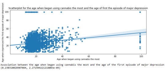
The scatterplot presented above, illustrates the correlation between the age when individuals began using cannabis the most (quantitative explanatory variable) and the age when they experienced the first episode of depression (quantitative response variable). The direction of the relationship is positive (increasing), which means that an increase in the age of cannabis use is associated with an increase in the age of the first depression episode. In addition, since the points are scattered about a line, the relationship is linear. Regarding the strength of the relationship, from the pearson correlation test we can see that the correlation coefficient is equal to 0.23, which indicates a weak linear relationship between the two quantitative variables. The associated p-value is equal to 2.27e-09 (p-value is written in scientific notation) and the fact that its is very small means that the relationship is statistically significant. As a result, the association between the age when began using cannabis the most and the age of the first depression episode is moderately weak, but it is highly unlikely that a relationship of this magnitude would be due to chance alone. Finally, by squaring the r, we can find the fraction of the variability of one variable that can be predicted by the other, which is fairly low at 0.05.

For the association between the age when individuals began using cannabis the most (quantitative explanatory variable) and the age when they experienced the first episode of anxiety (quantitative response variable), the scatterplot psented above shows a positive linear relationship. Regarding the strength of the relationship, the pearson correlation test indicates that the correlation coefficient is equal to 0.14, which is interpreted to a fairly weak linear relationship between the two quantitative variables. The associated p-value is equal to 0.0001, which means that the relationship is statistically significant. Therefore, the association between the age when began using cannabis the most and the age of the first anxiety episode is weak, but it is highly unlikely that a relationship of this magnitude would be due to chance alone. Finally, by squaring the r, we can find the fraction of the variability of one variable that can be predicted by the other, which is very low at 0.01.

0 notes

manju098 · 3 years ago

Text

Running a Chi-Square Test of Independence

import pandas import numpy import scipy.stats import seaborn import matplotlib.pyplot as plt

nesarc = pandas.read_csv ('nesarc_pds.csv' , low_memory=False)

Set PANDAS to show all columns in DataFrame

pandas.set_option('display.max_columns', None)

Set PANDAS to show all rows in DataFrame

pandas.set_option('display.max_rows', None)

nesarc.columns = map(str.upper , nesarc.columns)

pandas.set_option('display.float_format' , lambda x:'%f'%x)

Change my variables to numeric

nesarc['AGE'] = pandas.to_numeric(nesarc['AGE'], errors='coerce') nesarc['S3BQ4'] = pandas.to_numeric(nesarc['S3BQ4'], errors='coerce') nesarc['S3BQ1A5'] = pandas.to_numeric(nesarc['S3BQ1A5'], errors='coerce') nesarc['S3BD5Q2B'] = pandas.to_numeric(nesarc['S3BD5Q2B'], errors='coerce') nesarc['S3BD5Q2E'] = pandas.to_numeric(nesarc['S3BD5Q2E'], errors='coerce') nesarc['MAJORDEP12'] = pandas.to_numeric(nesarc['MAJORDEP12'], errors='coerce') nesarc['GENAXDX12'] = pandas.to_numeric(nesarc['GENAXDX12'], errors='coerce')

Subset my sample

subset1 = nesarc[(nesarc['AGE']>=18) & (nesarc['AGE']<=30)] # Ages 18-30 subsetc1 = subset1.copy()

subset2 = nesarc[(nesarc['AGE']>=18) & (nesarc['AGE']<=30) & (nesarc['S3BQ1A5']==1)] # Cannabis users, ages 18-30 subsetc2 = subset2.copy()

Setting missing data for frequency and cannabis use, variables S3BD5Q2E, S3BQ1A5

subsetc1['S3BQ1A5']=subsetc1['S3BQ1A5'].replace(9, numpy.nan) subsetc2['S3BD5Q2E']=subsetc2['S3BD5Q2E'].replace('BL', numpy.nan) subsetc2['S3BD5Q2E']=subsetc2['S3BD5Q2E'].replace(99, numpy.nan)

Contingency table of observed counts of major depression diagnosis (response variable) within cannabis use (explanatory variable), in ages 18-30

contab1=pandas.crosstab(subsetc1['MAJORDEP12'], subsetc1['S3BQ1A5']) print (contab1)

Column percentages

colsum=contab1.sum(axis=0) colpcontab=contab1/colsum print(colpcontab)

Chi-square calculations for major depression within cannabis use status

print ('Chi-square value, p value, expected counts, for major depression within cannabis use status') chsq1= scipy.stats.chi2_contingency(contab1) print (chsq1)

Contingency table of observed counts of geberal anxiety diagnosis (response variable) within cannabis use (explanatory variable), in ages 18-30

contab2=pandas.crosstab(subsetc1['GENAXDX12'], subsetc1['S3BQ1A5']) print (contab2)

Column percentages

colsum2=contab2.sum(axis=0) colpcontab2=contab2/colsum2 print(colpcontab2)

Chi-square calculations for general anxiety within cannabis use status

print ('Chi-square value, p value, expected counts, for general anxiety within cannabis use status') chsq2= scipy.stats.chi2_contingency(contab2) print (chsq2)

Contingency table of observed counts of major depression diagnosis (response variable) within frequency of cannabis use (10 level explanatory variable), in ages 18-30

contab3=pandas.crosstab(subset2['MAJORDEP12'], subset2['S3BD5Q2E']) print (contab3)

Column percentages

colsum3=contab3.sum(axis=0) colpcontab3=contab3/colsum3 print(colpcontab3)

Chi-square calculations for mahor depression within frequency of cannabis use groups

print ('Chi-square value, p value, expected counts for major depression associated frequency of cannabis use') chsq3= scipy.stats.chi2_contingency(contab3) print (chsq3)

recode1 = {1: 9, 2: 8, 3: 7, 4: 6, 5: 5, 6: 4, 7: 3, 8: 2, 9: 1} # Dictionary with details of frequency variable reverse-recode subsetc2['CUFREQ'] = subsetc2['S3BD5Q2E'].map(recode1) # Change variable name from S3BD5Q2E to CUFREQ

subsetc2["CUFREQ"] = subsetc2["CUFREQ"].astype('category')

Rename graph labels for better interpretation

subsetc2['CUFREQ'] = subsetc2['CUFREQ'].cat.rename_categories(["2 times/year","3-6 times/year","7-11 times/years","Once a month","2-3 times/month","1-2 times/week","3-4 times/week","Nearly every day","Every day"])

Graph percentages of major depression within each cannabis smoking frequency group

plt.figure(figsize=(12,4)) # Change plot size ax1 = seaborn.factorplot(x="CUFREQ", y="MAJORDEP12", data=subsetc2, kind="bar", ci=None) ax1.set_xticklabels(rotation=40, ha="right") # X-axis labels rotation plt.xlabel('Frequency of cannabis use') plt.ylabel('Proportion of Major Depression') plt.show()

Post hoc test, pair comparison of frequency groups 1 and 9, 'Every day' and '2 times a year'

recode2 = {1: 1, 9: 9} subsetc2['COMP1v9']= subsetc2['S3BD5Q2E'].map(recode2)

Contingency table of observed counts

ct4=pandas.crosstab(subsetc2['MAJORDEP12'], subsetc2['COMP1v9']) print (ct4)

Column percentages

colsum4=ct4.sum(axis=0) colpcontab4=ct4/colsum4 print(colpcontab4)

Chi-square calculations for pair comparison of frequency groups 1 and 9, 'Every day' and '2 times a year'

print ('Chi-square value, p value, expected counts, for pair comparison of frequency groups -Every day- and -2 times a year-') cs4= scipy.stats.chi2_contingency(ct4) print (cs4)

Post hoc test, pair comparison of frequency groups 2 and 6, 'Nearly every day' and 'Once a month'

recode3 = {2: 2, 6: 6} subsetc2['COMP2v6']= subsetc2['S3BD5Q2E'].map(recode3)

Contingency table of observed counts

ct5=pandas.crosstab(subsetc2['MAJORDEP12'], subsetc2['COMP2v6']) print (ct5)

Column percentages

colsum5=ct5.sum(axis=0) colpcontab5=ct5/colsum5 print(colpcontab5)

Chi-square calculations for pair comparison of frequency groups 2 and 6, 'Nearly every day' and 'Once a month'

print ('Chi-square value, p value, expected counts for pair comparison of frequency groups -Nearly every day- and -Once a month-') cs5= scipy.stats.chi2_contingency(ct5) print (cs5)

OUTPUT

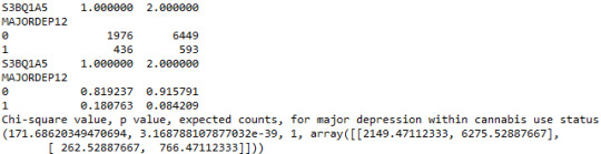
A Chi Square test of independence revealed that among cannabis users aged between 18 and 30 years old (subsetc2), the frequency of cannabis use (explanatory variable collapsed into 10 ordered categories) and past year depression diagnosis (response binary categorical variable) were significantly associated, X2 =35.18, 10 df, p=0.00011.

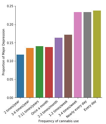
Similarly, the post hoc comparison (Bonferroni Adjustment) of rates of major depression by the pair of "Nearly every day” and “once a month” frequency categories, indicated that the p-value is 0.046 and the proportions of major depression diagnosis for each frequency group are 23.3% and 13.7% respectively. As a result, since the p-value is larger than the Bonferroni adjusted p-value (adj p-value = 0.05 / 45 = 0.0011<0.046), we can assume that these two rates are not significantly different from one another. Therefore, we accept the null hypothesis.

0 notes

manju098 · 3 years ago

Text

Running an analysis of variance

import pandas import numpy import statsmodels.formula.api as smf import statsmodels.stats.multicomp as multi nesarc = pandas.read_csv ('nesarc_pds.csv' , low_memory=False) # load NESARC dataset

Set PANDAS to show all columns in DataFrame

pandas.set_option('display.max_columns', None)

Set PANDAS to show all rows in DataFrame

pandas.set_option('display.max_rows', None)

nesarc.columns = map(str.upper , nesarc.columns)

pandas.set_option('display.float_format' , lambda x:'%f'%x)

Change my variables to numeric

nesarc['AGE'] = nesarc['AGE'].convert_objects(convert_numeric=True) nesarc['S3BQ4'] = nesarc['S3BQ4'].convert_objects(convert_numeric=True) nesarc['S3BQ1A5'] = nesarc['S3BQ1A5'].convert_objects(convert_numeric=True) nesarc['S3BD5Q2B'] = nesarc['S3BD5Q2B'].convert_objects(convert_numeric=True) nesarc['S3BD5Q2E'] = nesarc['S3BD5Q2E'].convert_objects(convert_numeric=True) nesarc['MAJORDEP12'] = nesarc['MAJORDEP12'].convert_objects(convert_numeric=True) nesarc['GENAXDX12'] = nesarc['GENAXDX12'].convert_objects(convert_numeric=True)

Subset my sample

subset5 = nesarc[(nesarc['AGE']>=18) & (nesarc['AGE']<=30) & (nesarc['S3BQ1A5']==1)] # Cannabis users, ages 18-30 subsetc5 = subset5.copy()

Setting missing data for quantity of cannabis (measured in joints), variable S3BQ4

subsetc5['S3BQ4']=subsetc5['S3BQ4'].replace(99, numpy.nan) subsetc5['S3BQ4']=subsetc5['S3BQ4'].replace('BL', numpy.nan)

sub1 = subsetc5[['S3BQ4', 'MAJORDEP12']].dropna()

Using ols function for calculating the F-statistic and the associated p value

Depression (categorical, explanatory variable) and joints quantity (quantitative, response variable) correlation

model1 = smf.ols(formula='S3BQ4 ~ C(MAJORDEP12)', data=sub1) results1 = model1.fit() print (results1.summary())

Measure mean and spread for categorical variable MAJORDEP12, major depression

print ('Means for joints quantity by major depression status') m1= sub1.groupby('MAJORDEP12').mean() print (m1)

print ('Standard deviations for joints quantity by major depression status') sd1 = sub1.groupby('MAJORDEP12').std() print (sd1)

sub2 = subsetc5[['S3BQ4', 'GENAXDX12']].dropna()

Using ols function for calculating the F-statistic and the associated p value

Anxiety (categorical, explanatory variable) and joints quantity (quantitative, response variable) correlation

model2 = smf.ols(formula='S3BQ4 ~ C(GENAXDX12)', data=sub2) results2 = model2.fit() print (results2.summary())

Measure mean and spread for categorical variable GENAXDX12, general anxiety

print ('Means for joints quantity by major general anxiety status') m2= sub2.groupby('GENAXDX12').mean() print (m2)

print ('Standard deviations for joints quantity by general anxiety status') sd2 = sub2.groupby('GENAXDX12').std() print (sd2)

Setting missing data for frequency of cannabis use, variable S3BD5Q2E

subsetc5['S3BD5Q2E']=subsetc5['S3BD5Q2E'].replace(99, numpy.nan) subsetc5['S3BD5Q2E']=subsetc5['S3BD5Q2E'].replace('BL', numpy.nan)

sub3 = subsetc5[['S3BQ4', 'S3BD5Q2E']].dropna()

Using ols function for calculating the F-statistic and associated p value

Frequency of cannabis use (10 level categorical, explanatory variable) and joints quantity (quantitative, response variable) correlation

model3 = smf.ols(formula='S3BQ4 ~ C(S3BD5Q2E)', data=sub3).fit() print (model3.summary())

Measure mean and spread for categorical variable S3BD5Q2E, frequency of cannabis use

print ('Means for joints quantity by frequency of cannabis use status') mc2= sub3.groupby('S3BD5Q2E').mean() print (mc2)

print ('Standard deviations for joints quantity by frequency of cannabis use status') sdc2 = sub3.groupby('S3BD5Q2E').std() print (sdc2)

Run a post hoc test (paired comparisons), using Tukey HSDT

mc1 = multi.MultiComparison(sub3['S3BQ4'], sub3['S3BD5Q2E']) res1 = mc1.tukeyhsd() print(res1.summary())

OUTPUT

In order to conduct post hoc paired comparisons in the context of my ANOVA, examining the association between frequency of cannabis use and number of joints smoked per day when using the most, I used the Tukey HSD test. The table presented above, illustrates the differences in smoking quantity for each cannabis use frequency group and help us identify the comparisons in which we can reject the null hypothesis and accept the alternate, that is, in which reject equals true. In cases where reject equals false, rejecting the null hypothesis resulting in inflating a type 1 error.

0 notes

manju098 · 3 years ago

Text

Creating graphs for your data

import pandas as pd import numpy as np import os import matplotlib.pyplot as plt import seaborn read pickled data data = pd.read_pickle('cleaned_data2.pickle') data.shape (43093, 12) data.dtypes

marital object age_1st_mar object age int64 hispanich int64 indian int64 asian int64 black int64 HAWAIIAN int64 WHITE int64 how_mar_ended object edu object ETHNICITY object dtype: object

data.head()

marital age_1st_mar age hispanich indian asian black HAWAIIAN WHITE how_mar_ended edu ETHNICITY

0 Never Married 23 1 2 2 2 2 1 Completed high school hispanich 1 Married 23 28 1 2 2 2 2 1 Completed high school hispanich 2 Widowed 35 81 1 2 2 2 2 1 2 8 hispanich 3 Never Married 18 1 2 2 2 2 1 Completed high school hispanich 4 Married 22 36 2 2 2 1 2 2 bachelor's black

%matplotlib inline barplot (count plot) for the marital status

univariate bar graph for categorical variables

First hange format from numeric to categorical

plt.figure(figsize=(15,5)) data["marital"] = data["marital"].astype('category')

seaborn.countplot(x="marital", data=data) plt.xlabel('marital ')

barplot (count plot) for the education level .

plt.figure(figsize=(18,8)) data["edu"] = data["edu"].astype('category')

seaborn.countplot(x="edu", data=data) plt.xlabel('education ')

barplot (count plot) for the ETHNICITY .

plt.figure(figsize=(10,5)) data["ETHNICITY"] = data["ETHNICITY"].astype('category')

seaborn.countplot(x="ETHNICITY", data=data) plt.xlabel('ETHNICITY ')

the distribution od the ages in the sample

plt.figure(figsize=(18,8)) seaborn.distplot(data["age"].dropna(), kde=False); plt.xlabel('Age')

plt.figure(figsize=(18,8))

seaborn.distplot(data["age_1st_mar"], kde=False);

plt.xlabel('age_1st_mar')

data.marital.describe()

count 43093 unique 6 top Married freq 20769 Name: marital, dtype: object

data['age_1st_mar'].describe()

count 43093 unique 59 top freq 10756 Name: age_1st_mar, dtype: object

data.age.describe()

count 43093.000000 mean 46.400808 std 18.178612 min 18.000000 25% 32.000000 50% 44.000000 75% 59.000000 max 98.000000 Name: age, dtype: float64

data.how_mar_ended.describe()

count 43093 unique 5 top freq 27966 Name: how_mar_ended, dtype: object renaming the education to be numeric and Representative for the estimate of years of studying .

edu_remap_dict = { 'No formal schooling':0, 'K, 1 or 2':1.5, '3 or 4':3.5, '5 or 6':5.5, '7':7, '8':8, '(grades 9-11)':10, 'Completed high school':12, ' degree':14, 'Some college (no degree)':14, 'technical 2-year degree':14, 'bachelor\'s':16, 'master\'s':18 }

data['edu'] = data['edu'].map(edu_remap_dict)

plt.figure(figsize=(12,8)) seaborn.factorplot(x="edu", y="age", data=data)

plt.xlabel('education') plt.ylabel('age at the first marriage') plt.title('the relationship between education and age at the first marriage ')

data.to_pickle('data.pickle') note there is two contentious numerical variables in the variables i chose that's why i didn't use scatter plots.

0 notes

manju098 · 3 years ago

Text

import pandas as pd import numpy as np import os import matplotlib.pyplot as plt import seaborn read data and pickle it all

this function reads data from csv file

def read_data(): data = pd.read_csv('/home/data-sci/Desktop/analysis/course/nesarc_pds.csv',low_memory=False)

return data

this function saves the data in a pickle "binary" file so it's faster to deal with it next time we run the script

def pickle_data(data): data.to_pickle('cleaned_data.pickle')

this function reads data from the binary .pickle file

def get_pickle(): return pd.read_pickle('cleaned_data.pickle') def the_data(): """this function will check and read the data from the pickle file if not fond it will read the csv file then pickle it""" if os.path.isfile('cleaned_data.pickle'): data = get_pickle()else: data = read_data() pickle_data(data) return data data = the_data() data.shape Out[21]: (43093, 3008) data.head() ETHRACE2A ETOTLCA2 IDNUM PSU STRATUM WEIGHT CDAY CMON CYEAR REGION … SOL12ABDEP SOLP12ABDEP HAL12ABDEP HALP12ABDEP MAR12ABDEP MARP12ABDEP HER12ABDEP HERP12ABDEP OTHB12ABDEP OTHBP12ABDEP 0 5 1 4007 403 3928.613505 14 8 2001 4 … 0 0 0 0 0 0 0 0 0 0 1 5 0.0014 2 6045 604 3638.691845 12 1 2002 4 … 0 0 0 0 0 0 0 0 0 0 2 5 3 12042 1218 5779.032025 23 11 2001 3 … 0 0 0 0 0 0 0 0 0 0 3 5 4 17099 1704 1071.754303 9 9 2001 2 … 0 0 0 0 0 0 0 0 0 0 4 2 5 17099 1704 4986.952377 18 10 2001 2 … 0 0 0 0 0 0 0 0 0 0 5 rows × 3008 columns data2 = data[['MARITAL','S1Q4A','AGE','S1Q4B','S1Q6A']] data2 = data2.rename(columns={'MARITAL':'marital','S1Q4A':'age_1st_mar', 'AGE':'age','S1Q4B':'how_mar_ended','S1Q6A':'edu'})

selecting the wanted range of values

#THE RANGE OF WANTED AGES

data2['age'] = data2[data2['age'] < 30] #THE RANGE OF WANTED AGES OF FISRT MARRIEGE

convert to numeric so we can subset the values < 25

data2['age_1st_mar'] = pd.to_numeric(data2['age_1st_mar'], errors='ignor') In [105]: data2 = data2[data2['age_1st_mar'] < 25 ] data2.age_1st_mar.value_counts() Out[105]: 21.0 3473 19.0 2999 18.0 2944 20.0 2889 22.0 2652 23.0 2427 24.0 2071 17.0 1249 16.0 758 15.0 304 14.0 150 Name: age_1st_mar, dtype: int64 for simplisity will remap the variable edu to have just 4 levels below high school education == 0 high school == 1 collage == 2 higher == 3 edu_remap ={1:0,2:0,3:0,4:0,5:0,6:0,7:0,8:1,9:1,10:1,11:1,12:2,13:2,14:3} data2['edu'] = data2['edu'].map(edu_remap) print the frquancy of the values def distribution(var_data): """this function will print out the frequency distribution for every variable in the data-frame """ #var_data = pd.to_numeric(var_data, errors='ignore') print("the count of the values in {}".format(var_data.name)) print(var_data.value_counts()) print("the % of every value in the {} variable ".format(var_data.name)) print(var_data.value_counts(normalize=True)) print("-----------------------------------")

def print_dist(): # this function loops though the variables and print them out for i in data2.columns: print(distribution(data2[i]))

print_dist() the count of the values in marital 1 13611 4 3793 3 3183 5 977 2 352 Name: marital, dtype: int64 the % of every value in the marital variable 1 0.621053 4 0.173070 3 0.145236 5 0.044579 2 0.016061

Name: marital, dtype: float64

None the count of the values in age_1st_mar 21.0 3473 19.0 2999 18.0 2944 20.0 2889 22.0 2652 23.0 2427 24.0 2071 17.0 1249 16.0 758 15.0 304 14.0 150 Name: age_1st_mar, dtype: int64 the % of every value in the age_1st_mar variable 21.0 0.158469 19.0 0.136841 18.0 0.134331 20.0 0.131822 22.0 0.121007 23.0 0.110741 24.0 0.094497 17.0 0.056990 16.0 0.034587 15.0 0.013871 14.0 0.006844

Name: age_1st_mar, dtype: float64

None the count of the values in age 1.0 1957 4.0 207 5.0 153 2.0 40 3.0 7 Name: age, dtype: int64 the % of every value in the age variable 1.0 0.827834 4.0 0.087563 5.0 0.064721 2.0 0.016920 3.0 0.002961

Name: age, dtype: float64

None the count of the values in how_mar_ended 10459 2 8361 1 2933 3 154 9 9 Name: how_mar_ended, dtype: int64 the % of every value in the how_mar_ended variable 0.477231 2 0.381502 1 0.133829 3 0.007027 9 0.000411

Name: how_mar_ended, dtype: float64

None the count of the values in edu 1 13491 0 4527 2 2688 3 1210 Name: edu, dtype: int64 the % of every value in the edu variable 1 0.615578 0 0.206561 2 0.122650 3 0.055211

Name: edu, dtype: float64

None summery

##### marital status

Married 0.48 % |

Living with someone 0.22 % |

Widowed 0.12 % |

Divorced 0.1 % |

Separated 0.03 % |

Never Married 0.03 % |

-------------------------------------|

##### AGE AT FIRST MARRIAGE FOR THOSE

WHO MARRY UNDER THE AGE OF 25 |

AGE % |

21 0.15 % |

19 0.13 % |

18 0.13 % |

20 0.13 % |

22 0.12 % |

23 0.11 % |

24 0.09 % |

17 0.05 % |

16 0.03 % |

15 0.01 % |

14 0.00 % |

-------------------------------------|

##### HOW FIRST MARRIAGE ENDED

Widowed 0.65 % |

Divorced 0.25 % |

Other 0.09 % |

Unknown 0.004% |

Na 0.002% |

-------------------------------------|

##### education

high school 0.58 % |

lower than high school 0.18 % |

collage 0.15 % |

ms and higher 0.07 % |

1- recoding unknown values from the variable "how_mar_ended" HOW FIRST MARRIAGE ENDED will code the 9 value from Unknown to NaN data2['how_mar_ended'] = data2['how_mar_ended'].replace(9, np.nan) data2['age_1st_mar'] = data2['age_1st_mar'].replace(99, np.nan) data2['how_mar_ended'].value_counts(sort=False, dropna=False) 1 4025 9 98 3 201 2 10803 27966 Name: how_mar_ended, dtype: int64

pickle the data tp binary .pickle file

pickle_data(data2)

0 notes