marindani11-blog

[marindani11-blog]

PREDICTING BLOOD DONATIONS BASED ON DONATION HISTORY

INTRODUCTION

 This study analyzes the history of donations to predict if a donor is likely to donate again within a given time window. Such estimate is based solely on donations patterns and history.

According to the American Red Cross, out of a potential pool of eligible blood donors in the Unites States of America (38 percent of the population) less than 10 percent actually donates each year. However, the demand is rather constant. Thus, it is crucial to understand the role donor history and past behavior plays in the probability of a person donating blood again. Then, the American Red Cross and other like institutions can use their existent database to call for donations in a particular time period; reducing costs and potentially increasing the number of future donations.

 METHODS

Sample

The data is provided by the UCI Machine Learning Repository; in the context of a DrivenData Competition. The sample included N= 576 donors selected at random from a blood transfusion service bus, owned by the Blood Transfusion Service Center in Hsin-Chu City, Taiwan. For each user Id, we have information on recentness, frequency, total volume of blood donated in c.c, time and whether he/she donated blood in March 2007.

Measures

The response variable is a categorical with two levels representing whether the donor donated blood in March 2007.

The predictors include 1) a measure of recentness given by the number of months past since the last donation, 2) the frequency is given by the total number of donations, 3) a measure of volume given by the total amount of blood donated in c.c. and 4) a measure of time given by the number of months past since the first donation.

Analyses

Since the explanatory variables are quantitative, the distributions were examined by computing numerical descriptions of the center and spread (standard deviation, mean, minimum and maximum values). The binary response variable is described by observing its frequency table.

The Analysis of Variance (ANOVA) will be use to test the associations between my explanatory variables and the two-level categorical response variable. More specifically, the ANOVA F test will show if the difference among sample means is really due to the variation within the groups or only due to sample variability.

Given the nature of the challenge, DataDriven provides a training data and test data. The training dataset contains N=576 and the test dataset has N= 200; no missing data is found in either dataset. The training dataset is used to fit the model that best predicts the value of the response variable; which is the subject of this project. Then I will use the test data to provide a probability for the last variable “Donations In March 2007”. Since I want to predict a log loss probability between 0 and 1 using only 4 quantitative predictors, I will fit a logistic regression model. This method is more robust given that the independent variables don’t have to be normally distributed, or have equal variance in each group. Also, logistic regressions do not assume a linear relationship.

Regarding data management for the model, I am creating a new variable displaying the time frame of the individual’s last blood donation. Thus: Time Frame = “Months Since First Donation" - "Months Since Last Donation".  From the descriptive and bivariate analysis, we can see a strong correlation between the number of donations and the total volume of blood collected; therefore I am dropping the latter.  I will center each variable to account for the differences in distribution (and obtain residuals that are approximately symmetrically distributed).

 Finally, I will conclude the analysis with the calculation of odd ratios.

RESULTS - Descriptive Statistics

The explanatory variable is binary were 1 means the person made a blood donation in March 2007 (N=138, Frequency =23,9%), and 0 otherwise (N=438, Frequency = 76%).

The following table displays the descriptive statistics for the explanatory variables.

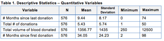
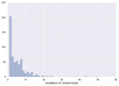
From this analysis we can see that the overall data has been taken in a period of 8 years, with the newest people participating started donating blood 2 months prior to the data collection. We also learned that the average donor gave 1356 c.c. and donated about 5 times, the last time being 9.44 months. The total number of donations has a standard deviation of 5.74. Figure 1 provides a closer look at the distribution of the number of donations variable.

Figure 1. Distribution of Total Number of Donations

[marindani11-blog]

LOGIT REGRESSION MODEL

DATA MANAGEMENT

I have decided to work with the National Longitudinal Study of Adolescent to Adult Health (Add Health) dataset. The response variable is the adolescent’s grades in school, with 1 indicated they have a passing grade. My explanatory variable is a binary variable reflecting the mother’s level of education with value 1 if she has completed high school of higher levels of education.Lastly, I added a control variable indicating the mother’s presence in the household with a value of 1 if the mother is at home before and after the son/daughter’s school; and 0 otherwise. 

MODEL AND RESULTS

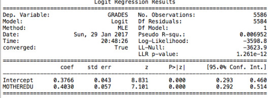
The first regression I tested is the relation between grades (pass/fail) and the level of mother’s education. The following table clearly shows that there is a significant positive correlation (p value is lower than 0.05).  

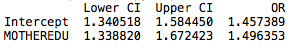
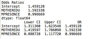
Adolescents in  my sample with a mother that is at least high school educated are 1.5 times more likely to have a passing grade. The confidence intervals tells us that there is a 95% chance that the odds ratio falls between 1.34 and 1.67.

Then, I decided to include a control variable to measure the effect that the mother’s presence in the household has on grades. After running the regression, we still have a significant correlation of mother’s education level with grades. However, the mother’s presence in a household is not significant (p value higher than 0.05).  

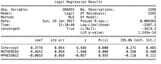
Adolescents are 1.6 times more likely to pass their exams with high school educated mothers, after controlling for mother's presence in the household. Furthermore, adolescents that have their mother's present in the house are equally likely to pass their exams (odd ratio very close to 1); however this relation is not significant in my sample.

CODE

@author: marindani11 """ import pandas import numpy import scipy.stats import statsmodels.formula.api as smf import statsmodels.api as sm import statsmodels.stats.multicomp as multi import seaborn import matplotlib.pyplot as plt import pickle

rawdata = pandas.read_csv("/Users/marindani11/Desktop/Coursera/SPECIALIZATION/Python/addhealth_pds.csv",low_memory=False)

#Collapse response variables into only 2 values : Pass / fail rawdata['H1ED11'] = rawdata['H1ED11'].convert_objects(convert_numeric=True) rawdata['H1ED12'] = rawdata['H1ED12'].convert_objects(convert_numeric=True) rawdata['H1ED13'] = rawdata['H1ED13'].convert_objects(convert_numeric=True) rawdata['H1ED14'] = rawdata['H1ED14'].convert_objects(convert_numeric=True)

def GRADES (row):   if row['H1ED11' and 'H1ED12' and 'H1ED13' and 'H1ED14'] == 1 :      return 1   elif row['H1ED11' and 'H1ED12' and 'H1ED13' and 'H1ED14'] ==2 :      return 1   elif row['H1ED11' and 'H1ED12' and 'H1ED13' and 'H1ED14'] ==3 :      return 0   elif row['H1ED11' and 'H1ED12' and 'H1ED13' and 'H1ED14'] ==4 :      return 0

rawdata['GRADES'] = rawdata.apply (lambda row: GRADES (row),axis=1)

#Mother's education rawdata['H1RM1']=rawdata['H1RM1'].convert_objects(convert_numeric=True) rawdata['MEDU'] = rawdata['H1RM1'].replace([11,12,96,97,98], numpy.nan) rawdata['MEDU'] = rawdata['MEDU'].dropna() def MOTHEREDU (row):   rawdata['H1RM1']=rawdata['H1RM1'].dropna()   if row['H1RM1'] >4 :      return 1   elif row['H1RM1'] <=4 :      return 0

rawdata['MOTHEREDU'] = rawdata.apply (lambda row: MOTHEREDU (row),axis=1) rawdata['MOTHEREDU'].value_counts(sort=False)

#Presence in the household #Create a binary variable as a proxy for mother's presence in the household rawdata['H1RM12']=rawdata['H1RM12'].convert_objects(convert_numeric=True) rawdata['H1RM12'] = rawdata['H1RM12'].replace([96,97,98,99], numpy.nan)

def MPRESENCE (row):   rawdata['H1RM12']=rawdata['H1RM12'].dropna()   if row['H1RM12']<=2 :      return 1   elif row['H1RM12'] ==3 :      return 0   elif row['H1RM12'] == 4 :      return 0   elif row['H1RM12'] == 5 :      return 0   elif row['H1RM12'] == 6 :      return 1

rawdata['MPRESENCE'] = rawdata.apply (lambda row: MPRESENCE (row),axis=1) rawdata['MPRESENCE'].value_counts(sort=False)

#Logistic regression mother's education lreg1=smf.logit(formula='GRADES ~ MOTHEREDU', data=rawdata).fit() print(lreg1.summary())

#odds ratios print("Odds Ratios") print(numpy.exp(lreg1.params))

#Confidence intervals for odds ratios params=lreg1.params conf=lreg1.conf_int() "returns the confidence intervals for the parameter estimates" conf['OR']=params conf.columns=['Lower CI','Upper CI', 'OR'] print(numpy.exp(conf))

#Logistic regression mother's education controlling for her presence in the hh lreg2=smf.logit(formula='GRADES ~ MOTHEREDU + MPRESENCE', data=rawdata).fit() print(lreg2.summary())

#odds ratios print("Odds Ratios") print(numpy.exp(lreg2.params))

#Confidence intervals for odds ratios params=lreg2.params conf=lreg2.conf_int() "returns the confidence intervals for the parameter estimates" conf['OR']=params conf.columns=['Lower CI','Upper CI', 'OR'] print(numpy.exp(conf))

[marindani11-blog]

MULTIPLE REGRESSION ANALYSIS

DATA MANAGEMENT

For this week assignment I decided to run a multiple regression model testing the association between marijuana use over lifetime (response variable) and a measure of violent behavior (explanatory variable) while controlling for parental control, parental level of education, presence of an adult in the household and other usage of drugs .  In order to do it I used the AddHealth data.

All the quantitative variables were standardized to have a mean of 0 and standard deviation of 1.

MODEL

After running a basic OLS function, we can see that the model is under-fitted since the explanatory variables only explain 10,4% (r-squared) of the variance of marijuana use; even though the model is significant (p-value =0,0116).

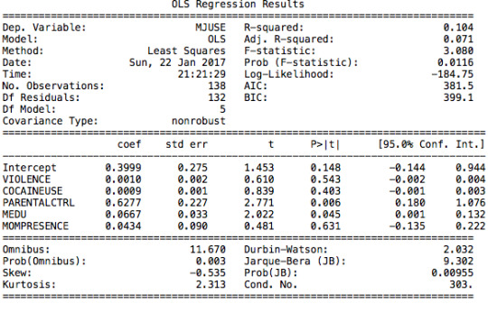
The model does not allow us to reject the null hypothesis since the coefficient for violence is not significant. The use of cocaine is positively correlated to marijuana use, yet not significant either. We can say the same for presence of an adult. Yet, parental control and mother’s education have significant coefficients with an interval of confidence that oscillates from 0,18 to 1,08 ; and 0,001 to 0,13 respectively.

MISSPECIFICATION

To verify if the model is correctly specified, I will run a series of studies on the residuals.

1) qq plot

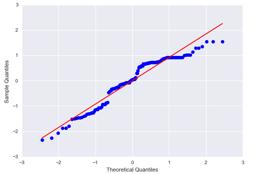
The plot shows that the error terms do not follow a perfect normal distribution; therefore the model is not correctly specified. We will dig deeper to see the probable reasons for it.

2) Standardize errors 

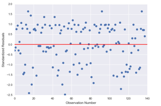
The figure shows us that 95% of the residuals fall between 2 and -2 intervals. However, we do see some error terms close to the -2,5 interval. This means we have some outliers in the data but they’re not extreme outliers. Thus, the shortcuts of the model can be attributed to important explanatory variables missing.

3) Leverage plot

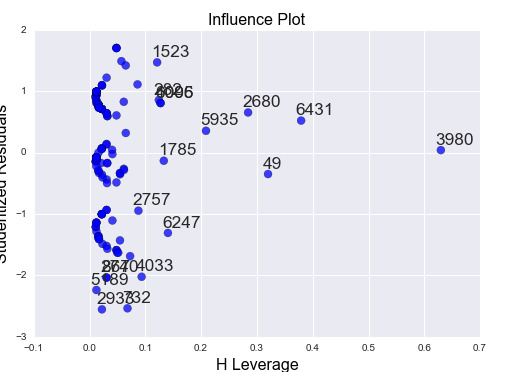
This plot confirms that there are a few outliers but with a small leverage value (close to 0). We can also see that there is a higher than average leverage observation that isn’t an outlier.

CODE

@author: marindani11 """

import pandas import numpy import scipy.stats import statsmodels.formula.api as smf import statsmodels.api as sm import statsmodels.stats.multicomp as multi import seaborn import matplotlib.pyplot as plt import pickle

#import sub2 rawdata = pandas.read_csv("/Users/marindani11/Desktop/Coursera/SPECIALIZATION/Python/addhealth_pds.csv",low_memory=False)

#OLS REGRESSION

ols4 = smf.ols(formula='MJUSE ~ VIOLENCE + COCAINEUSE + PARENTALCTRL +  MEDU +  MOMPRESENCE', data=rawdata).fit() print(ols4.summary())

############ MISSPECIFICATION ############ "if a model is correctly specified, then the residuals are not correlated with the explanatroy variables"

#qqplot fig1=sm.qqplot(ols4.resid,line='r') "to check if the residuals are normally distributed"

#standardize residuals stdres=pandas.DataFrame(ols4.resid_pearson) fig2=plt.plot(stdres,'o',ls='None') l=plt.axhline(y=0, color='r') plt.ylabel('Standardized Residuals') plt.xlabel('Observation Number') print(fig2) "to check if the standardize errors fit a normal distribution" "95% of the residuals to fall between 2 std of the mean" "no data outside the 2.5 interval so no extreme outliers"

#leverage plot fig3=sm.graphics.influence_plot(ols4,size=8) print(fig3) "identify observations that have an unusually large influence on the predicted value estimate" "we can also see if there are any outliers (residuals greater than 2 or less -2)" "small or close to 0 leverage values of the outliers shown -2)" "higher than average leverage but not an outlier"

[marindani11-blog]

K-MEANS CLUSTER ANALYSIS

DATA MANAGEMENT

For this week’s assignment I ran a k-mean cluster analysis to identify subgroups of adolescents based on 14 variables representing (gender) Male; (race/ethnicity) Hispanic, White, Black, Native American and Asian; (parent’s education level) mother’s level of education and father’s level of education; (extracurricular activities) time spent watching tv, time spent in sports and whether the student has a job; Use of other drugs and (academic behavior) grades and years expelled from school. All clustering variables were standardized to have a mean of 0 and standard deviation of 1.

MODEL

I specified k = 1 to 9 clusters and a series of k-means cluster analyses were conducted using Euclidean distance. The variance in the clustering variables was plotted for each of the cluster solutions (1 to 9) in an elbow curve to provide guidance for choosing the number of clusters to interpret.

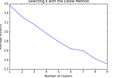
The results could be interpreted of a 6-cluster solution. Thus, I ran the analysis again limiting k to 6. I plotted the first two canonical variables for the clustering variables by cluster (represented by color).

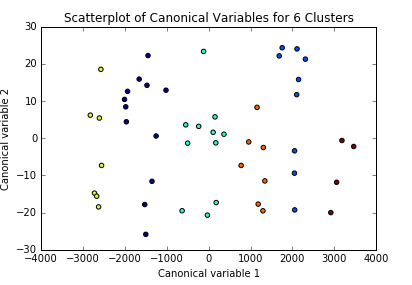
Initially, we can think the clusters are well represented since they don’t seem to be overlapping.  I analyzed it further by comparing the means on the clustering variables, compared to other clusters.

Following up, I tested the validity of the clusters with an analysis of variance (ANOVA). I tested for significant differences between the clusters on violence levels (measured as the number of times the person was in a fight during the past year). A tukey test was used for post hoc comparisons between the clusters. Results indicated significant differences between the clusters on violence ( p<.0001). The tukey post hoc comparisons, however did not showed significant differences between clusters on violence levels,  with the exception that clusters 1 and 2 that were significantly different from each other.

Adolescents in cluster 1 had the highest violence levels (mean=3,84, sd=0.4), and cluster 2 had the lowest violence levels (mean=0.2, sd=0.7). In cluster 1 we have the group of adolescents with the lowest parental level of education (for both parents) and the highest probability of being expelled from school. 

CODE

@author: marindani11 """ import pandas as pd from pandas import Series from pandas import DataFrame import numpy as np import matplotlib.pylab as plt import pickle from sklearn.cross_validation import train_test_split from sklearn import preprocessing from sklearn.cluster import KMeans from scipy.spatial.distance import cdist from sklearn.decomposition import PCA import statsmodels.formula.api as smf import statsmodels.stats.multicomp as multi

#IMPORT DATA PREVIOUSLY CLEANED FOR THIS EXCERCISE with open('decisionTree.pickle', 'rb') as data:    dataset = pickle.load(data)

#DATA MANAGEMENT #Create 2 data sets: 1 includes only the predictor variables, # 2 includes the response variable recode1 = {1:1, 2:0} dataset['MALE']= dataset['BIO_SEX'].map(recode1)

#violence dataset['VIOLENCE']=dataset['H1FV13'].convert_objects(convert_numeric=True) dataset['VIOLENCE'] = dataset['VIOLENCE'].replace([996,997,998,999], np.nan) dataset['VIOLENCE']=dataset['VIOLENCE'].dropna()

#Marijuana Use over lifetime dataset['MJUSE']=dataset['H1TO33'].convert_objects(convert_numeric=True) dataset['MJUSE'] = dataset['MJUSE'].replace([996,997,998,999], np.nan) dataset['MJUSE']=dataset['MJUSE'].dropna()

#Alcohol Use over past year dataset['ALCOHOLUSE']=dataset['H1TO16'].convert_objects(convert_numeric=True) dataset['ALCOHOLUSE'] = dataset['ALCOHOLUSE'].replace([996,997,998,999], np.nan) dataset['ALCOHOLUSE']=dataset['ALCOHOLUSE'].dropna()

#Expelled from school dataset['EXPELLED']=dataset['H1ED9'].convert_objects(convert_numeric=True) dataset['EXPELLED']=dataset['EXPELLED'].replace([6,8], np.nan) dataset['EXPELLED']=dataset['EXPELLED'].dropna()

#Clean the dataset dataset=dataset.dropna()

#SELECT PREDICTORS cluster=dataset[['LATINOS', 'WHITE','BLACK','AMINDIAN','ASIAN','MOTHEREDU', 'FATHEREDU','TVTIME','SPORTSTIME','JOB','MJUSE','MALE','EXPELLED','GRADES']]

cluster.describe()

#Predictors need to be standardize so they're comparable. #Standardization of mean = 0; standard deviation= 1 #dataset=dataset.dropna() clustervar=cluster.copy() "the preprocessing.scale function transform the variable into one with mean 0 and stdv 1" "float64 ensures the variables have a numeric format" clustervar['LATINOS']=preprocessing.scale(clustervar['LATINOS'].astype('float64')) clustervar['WHITE']=preprocessing.scale(clustervar['WHITE'].astype('float64')) clustervar['BLACK']=preprocessing.scale(clustervar['BLACK'].astype('float64')) clustervar['AMINDIAN']=preprocessing.scale(clustervar['AMINDIAN'].astype('float64')) clustervar['ASIAN']=preprocessing.scale(clustervar['ASIAN'].astype('float64')) clustervar['MOTHEREDU']=preprocessing.scale(clustervar['MOTHEREDU'].astype('float64')) clustervar['FATHEREDU']=preprocessing.scale(clustervar['FATHEREDU'].astype('float64')) clustervar['TVTIME']=preprocessing.scale(clustervar['TVTIME'].astype('float64')) clustervar['SPORTSTIME']=preprocessing.scale(clustervar['SPORTSTIME'].astype('float64')) clustervar['JOB']=preprocessing.scale(clustervar['JOB'].astype('float64')) clustervar['MJUSE']=preprocessing.scale(clustervar['MJUSE'].astype('float64')) clustervar['MALE']=preprocessing.scale(clustervar['MALE'].astype('float64')) clustervar['EXPELLED']=preprocessing.scale(clustervar['EXPELLED'].astype('float64')) #clustervar['PARENTALCTRL']=preprocessing.scale(clustervar['PARENTALCTRL'].astype('float64')) #clustervar['COCAINEUSE']=preprocessing.scale(clustervar['COCAINEUSE'].astype('float64')) clustervar['GRADES']=preprocessing.scale(clustervar['GRADES'].astype('float64'))

# split data into train and test sets clus_train, clus_test = train_test_split(clustervar, test_size=.3, random_state=123) "random datasets with 70%/30% of the data"

#MODEL # k-means cluster analysis "we don't know how many clusters may be optimal, so we create an array of numbers between 1 and 10" clusters= range(1,10) "this will give us the cluster solutions for k=1 and k=9 when we test it" meandist=[] "it will be use to store the average distance values that will calculate for each k 1 to 9"

for k in clusters:    model=KMeans(n_clusters=k)    model.fit(clus_train)    clusassign=model.predict(clus_train)    meandist.append(sum(np.min(cdist(clus_train,model.cluster_centers_, 'euclidean'),axis=1))/clus_train.shape[0]) "for each value of k between 1 to 9,n_clusters indicates the # of clusters" "clusassign stores, for each observation, the cluster number to which it was assigned based on the cluster analysis" "model.predict is use to store the closest cluster that each observation belongs to." "then we calculate the average distance between each observation and the cluster centeroids." "we use the np.min function to calculate the smallest (minimum) difference for each observation among cluster centroids" "then we use the sum function to sum the minimum distances across all observations." "he / clus_train.shape with 0 in brackets divides the sum of the distances by the number of observations in the " "clus_train data set where the .shape with 0 in brackets code returns the number of observations in the clus_train data set."

#VISUALIZATION # plot average distance from observations from the cluster centroid "we use the Elbow Method to identify number of clusters to choose." plt.plot(clusters,meandist) plt.xlabel('Number of clusters') plt.ylabel('Average distance') plt.title('Selecting k with the Elbow Method')

#We saw the bend in cluster #8, so we'll re run the analysis model6=KMeans(n_clusters=6) model6.fit(clus_train) clausassign=model6.predict(clus_train)

"use canonical discriminant analysis that creates smaller number of variables, so we can plot in a p dimension" pca_2=PCA(2) "returns 2 best canonical variables" plot_columns=pca_2.fit_transform(clus_train) "asks python to fit the clusters into canonical variables" plt.scatter(x=plot_columns[:,0],y=plot_columns[:,1], c=model6.labels_,) plt.xlabel('Canonical variable 1') plt.ylabel('Canonical variable 2') plt.title('Scatterplot of Canonical Variables for 6 Clusters') plt.show()

#Pattern of means on the clustering variables for each cluster to see whether they are distinct and meaningful "create a unique identifier variable for clus train dataset that has the clustering variables" clus_train.reset_index(level=0,inplace=True) cluslist=list(clus_train['index']) labels=list(model6.labels_) "list of the cluster assignment for each observation" "combine both lists into a directory: dict command creates dictionary, zip command combines lists" newlist=dict(zip(cluslist,labels)) "convert the dictionary into a dataframe" newclus=DataFrame.from_dict(newlist,orient='index') "rename the cluster assignment column" newclus.columns=['cluster'] "create a unique identifier for the cluster assignment to merge with cluster training data" newclus.reset_index(level=0, inplace=True) "merge cluster assignment dataframe with cluster training variable datafrem by index variable" merged_train=pd.merge(clus_train,newclus,on='index') "on=index matches them by index" merged_train.head(n=100) "Calculate clustering variables by cluster" clustergrp=merged_train.groupby('cluster').mean() print("Clustering variable means by cluster") print(clustergrp)

#Test clusters with respect of violent behaviour

violence_data=dataset['VIOLENCE'] violence_train, violence_test=train_test_split(violence_data,test_size=.3,random_state=123) violence_train1=pd.DataFrame(violence_train) violence_train1.reset_index(level=0,inplace=True) merged_train_all=pd.merge(violence_train1,merged_train,on='index') sub1=merged_train_all[['VIOLENCE','cluster']].dropna()

#use analysis of variance to see if there are significant differences between clusters on violence levels violmod = smf.ols(formula='VIOLENCE ~ C(cluster)', data=sub1).fit() print (violmod.summary())

print ('means for violence by cluster') m1= sub1.groupby('cluster').mean() print (m1)

print ('standard deviations for violence by cluster') m2= sub1.groupby('cluster').std() print (m2)

#Tukey test to evaluate post hoc comparisons btw clusters using multi comparison function mc1 = multi.MultiComparison(sub1['VIOLENCE'], sub1['cluster']) res1 = mc1.tukeyhsd() print(res1.summary())

[marindani11-blog]

LASSO REGRESSION

I ran a lasso regression to identify a subset of variables from a pool of 14 variables that best predict a quantitative response variable measuring alcohol use amongst American Adolescents.  The list of predictors are: (gender) Male; (race/ethnicity) Hispanic, White, Black, Native American and Asian; (parent’s education level) mother’s level of education and father’s level of education; (extracurricular activities) time spent watching tv, time spent in sports and whether the student has a job; Use of other drugs and (academic behavior) grades and years expelled from school.

In order to compare, I standardize all variables to a mean equal to 0 and standard deviation of 1.

 MODEL DESCRIPTION AND RESULTS 

The best fitted model for the training data predicted the following: 

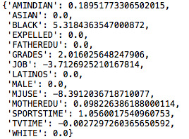
Among the 14 variables, the model retained 8 of them. The model estimates that American Indians, African Americans, having failing grades and not being involved in sports has a positive correlation to alcohol use. While Marijuana use and time spent watching tv are negatively correlated.

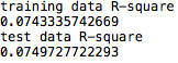
However, these 8 variables only account for 7% of the variance for both the training and test data.

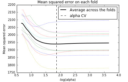
The change in the cross validation average (mean) squared error at each step was used to identify the best subset of predictor variables.

CODE

import numpy as np import matplotlib.pylab as plt import pickle from sklearn.cross_validation import train_test_split from sklearn.linear_model import LassoLarsCV

#IMPORT DATA PREVIOUSLY CLEANED FOR THIS EXCERCISE with open('decisionTree.pickle', 'rb') as data:    dataset = pickle.load(data)

#DATA MANAGEMENT #Create 2 data sets: 1 includes only the predictor variables, # 2 includes the response variable recode1 = {1:1, 2:0} dataset['MALE']= dataset['BIO_SEX'].map(recode1)

#Marijuana Use over lifetime dataset['MJUSE']=dataset['H1TO33'].convert_objects(convert_numeric=True) dataset['MJUSE'] = dataset['MJUSE'].replace([996,997,998,999], np.nan) dataset['MJUSE']=dataset['MJUSE'].dropna()

#Alcohol Use over past year dataset['ALCOHOLUSE']=dataset['H1TO16'].convert_objects(convert_numeric=True) dataset['ALCOHOLUSE'] = dataset['ALCOHOLUSE'].replace([996,997,998,999], np.nan) dataset['ALCOHOLUSE']=dataset['ALCOHOLUSE'].dropna()

#Expelled from school dataset['EXPELLED']=dataset['H1ED9'].convert_objects(convert_numeric=True) dataset['EXPELLED']=dataset['EXPELLED'].replace([6,8], np.nan) dataset['EXPELLED']=dataset['EXPELLED'].dropna()

#SELECT PREDICTORS predictorsvar=dataset[['LATINOS', 'WHITE','BLACK','AMINDIAN','ASIAN','MOTHEREDU', 'FATHEREDU','TVTIME','SPORTSTIME','JOB','MJUSE','MALE','GRADES','EXPELLED']]

targets = dataset.ALCOHOLUSE

#Predictors need to be standardize so they're comparable. #Standardization of mean = 0; standard deviation= 1 #dataset=dataset.dropna() predictors=predictorsvar.copy() from sklearn import preprocessing "the preprocessing.scale function transform the variable into one with mean 0 and stdv 1. "

predictors['LATINOS']=preprocessing.scale(predictors['LATINOS'].astype('float64')) predictors['WHITE']=preprocessing.scale(predictors['WHITE'].astype('float64')) predictors['BLACK']=preprocessing.scale(predictors['BLACK'].astype('float64')) predictors['AMINDIAN']=preprocessing.scale(predictors['AMINDIAN'].astype('float64')) predictors['ASIAN']=preprocessing.scale(predictors['ASIAN'].astype('float64')) predictors['MOTHEREDU']=preprocessing.scale(predictors['MOTHEREDU'].astype('float64')) predictors['FATHEREDU']=preprocessing.scale(predictors['FATHEREDU'].astype('float64')) predictors['TVTIME']=preprocessing.scale(predictors['TVTIME'].astype('float64')) predictors['SPORTSTIME']=preprocessing.scale(predictors['SPORTSTIME'].astype('float64')) predictors['JOB']=preprocessing.scale(predictors['JOB'].astype('float64')) predictors['MJUSE']=preprocessing.scale(predictors['MJUSE'].astype('float64')) predictors['MALE']=preprocessing.scale(predictors['MALE'].astype('float64')) predictors['GRADES']=preprocessing.scale(predictors['GRADES'].astype('float64')) predictors['EXPELLED']=preprocessing.scale(predictors['EXPELLED'].astype('float64')) # split data into train and test sets pred_train, pred_test, tar_train, tar_test = train_test_split(predictors, targets, test_size=.3, random_state=123) "random datasets with 70%/30% of the data"

#MODEL # specify the lasso regression model "to fit the model in the training set: .fit(pred_train, tar_train)" model=LassoLarsCV(cv=10, precompute=False).fit(pred_train,tar_train)

#Ask python to print the variable names and regression coefficients from best suitable model. # print variable names and regression coefficients dict(zip(predictors.columns, model.coef_)) "dict creates a dictionary, zip creates a list"

#VISUALIZATION # plot coefficient progression m_log_alphas = -np.log10(model.alphas_) ax = plt.gca() plt.plot(m_log_alphas, model.coef_path_.T) plt.axvline(-np.log10(model.alpha_), linestyle='--', color='k',            label='alpha CV') plt.ylabel('Regression Coefficients') plt.xlabel('-log(alpha)') plt.title('Regression Coefficients Progression for Lasso Paths')

"alphas in the sklearn library refers to the lambda. We use log of alpha for easier visualization" "plt.plot asks python to plot the log of alphas in the x axis and the regression coefs in the y axis" "plt.axvline function to plot the transformed values"

#plot mean squred error for change in the parameter alpha m_log_alphascv = -np.log10(model.cv_alphas_) plt.figure() plt.plot(m_log_alphascv, model.cv_mse_path_, ':') plt.plot(m_log_alphascv, model.cv_mse_path_.mean(axis=-1), 'k',         label='Average across the folds', linewidth=2) plt.axvline(-np.log10(model.alpha_), linestyle='--', color='k',            label='alpha CV') plt.legend() plt.xlabel('-log(alpha)') plt.ylabel('Mean squared error') plt.title('Mean squared error on each fold') "we are using the mean square error for each cross validation fold (cv): model.cv_mse_path" "column in quotes in the attributes of plot function tells python to use dotted lines"

#plot the rsquare (proportion of variance) from training and test data. # MSE from training and test data

[marindani11-blog]

BASIC LINEAR REGRESSION

For this week assignment I decided to run a basic regression testing the association between cocaine use over lifetime (response variable) and a measure of parental control (explanatory variable).  In order to do it I used the AddHealth data.

DATA MANAGEMENT

The response variable is a measure of usage of cocaine over the adolescent’s lifetime, quantitative variable. My explanatory variable is a binary variable with value 1 if a) the parents does not set the adolescent’s curfew over the weekends and b) parents does not control the people their child hangs with; and 0 otherwise. 

MODEL

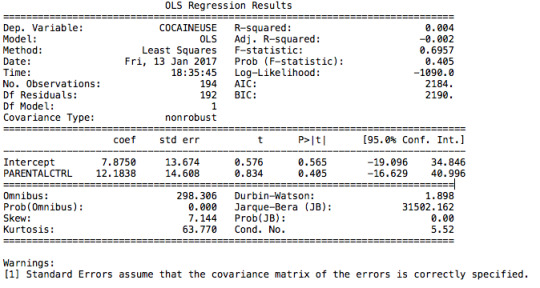
After running a basic OLS function, we can see that the model is under-fitted with a very low R-squared value (0,4%) and a p value of 0,405. Thus the relation is not significant.  The regression coefficient is 12.18, which means that the model predicts that an adolescent without parental would smoke 12.18 times more than a peer with parental control.

 The shortcuts of the model can have various explanations:

Cocaine use is misrepresented as adolescents can underreport their drug use due to social prejudice;

The explanatory variable does not capture parental control since we can’t measure the efficiently of such restrictions. Can parents enforce it? Are the parents present in the household?

Other variables can play an integral role in the adolescent behavior that we are not capturing in this bivariate model. We need to introduce some control variables.

CODE

#Import libraries import pandas import numpy import scipy.stats import statsmodels.formula.api as smf import statsmodels.stats.multicomp as multi import seaborn import matplotlib.pyplot as plt import pickle

#import sub2 rawdata = pandas.read_csv("/Users/marindani11/Desktop/Coursera/SPECIALIZATION/Python/addhealth_pds.csv",low_memory=False)

""" ----- DATA MANAGEMENT ----"""

#EXPLANATORY VARIABLE: Parental Control 

rawdata['H1WP2']=rawdata['H1WP2'].convert_objects(convert_numeric=True) rawdata['H1WP2']=rawdata['H1WP2'].replace([6,7,8,9],numpy.nan) rawdata['H1WP2']=rawdata['H1WP2'].dropna()

rawdata['H1WP1']=rawdata['H1WP1'].convert_objects(convert_numeric=True) rawdata['H1WP1']=rawdata['H1WP1'].replace([6,7,8,9],numpy.nan) rawdata['H1WP1']=rawdata['H1WP1'].dropna()

rawdata['H1WP3']=rawdata['H1WP3'].convert_objects(convert_numeric=True) rawdata['H1WP3']=rawdata['H1WP3'].replace([6,7,8,9],numpy.nan) rawdata['H1WP3']=rawdata['H1WP3'].dropna()

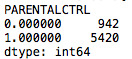
def PARENTALCTRL (row):   if row['H1WP1'and'H1WP2'] ==0:      return 0   elif row['H1WP1'and'H1WP2'] ==1 :      return 1

rawdata['PARENTALCTRL'] = rawdata.apply (lambda row: PARENTALCTRL (row),axis=1) g1= rawdata.groupby('PARENTALCTRL').size() print (g1) rawdata['PARENTALCTRL'].value_counts(sort=False)

#RESPONSE VARIABLE: Cocaine use in lifetime rawdata['COCAINEUSE']=rawdata['H1TO35'].convert_objects(convert_numeric=True) rawdata['COCAINEUSE'] = rawdata['COCAINEUSE'].replace([996,997,998,999], numpy.nan) rawdata['COCAINEUSE']=rawdata['COCAINEUSE'].dropna()

CocaineUseDesc=rawdata['COCAINEUSE'].value_counts(sort=False) print(CocaineUseDesc)

""" ---- OLS REGRESSION ---- """

ols1 = smf.ols(formula='COCAINEUSE ~ PARENTALCTRL', data=rawdata).fit() print(ols1.summary())

[marindani11-blog]

RANDOM FORESTS

THE DATA

I ran a random forest analysis to test the nonlinear relationships among the students performances (measured with a binary variable of pass/fail grades in various subjects) and the following explanatory variables: (race/ethnicity) Hispanic, White, Black, Native American and Asian; (parent’s education level) mother’s level of education and father’s level of education; (extracurricular activities) time spent watching tv, time spent in sports and whether the student has a job. 

 THE MODEL

The classification model’s accuracy was fairly low, with only 63,5% test score. This might be due to the exclusion of some key explanatory variables that I’ll include going forward. I also try to improve accuracy by controlling the parameter of the classifier; and I’m currently presenting the best option. The following table displays the importance scores (features) for each of my variables: 

Thus, test scores are not correlated to race but rather to the parent’s level of education (mother’s being the highest feature) and time spent doing extracurricular activities. Furthermore, while testing for the optimal number of trees, we can see that the strongest signals emerge while growing the forest but that with 1 tree the test score is already near the highest rate (63,5%). 

Note: Going forward I’ll optimize my model by adding more/better explanatory variables.

CODE

from pandas import Series, DataFrame import pandas as pd import numpy as np import os import matplotlib.pylab as plt from sklearn.cross_validation import train_test_split from sklearn.tree import DecisionTreeClassifier from sklearn.metrics import classification_report import sklearn.metrics import pickle

#IMPORT DATA PREVIOUSLY CLEANED FOR THIS EXCERCISE with open('decisionTree.pickle', 'rb') as data:    dataset = pickle.load(data)

dataset.dtypes dataset.describe()

# SET RESPONSIVE AND EXPLANATORY VARIABLES predictors=dataset[['LATINOS', 'WHITE','BLACK','AMINDIAN','ASIAN','MOTHEREDU', 'FATHEREDU','TVTIME','SPORTSTIME','JOB']]

targets = dataset.GRADES

#INDICATE THE SIZE OF DATA SAMPLES FOR TRAINING AND TESTING "test_size indicates the % we want -  in this case 60% training sample, 40% test sample" pred_train, pred_test, tar_train, tar_test  =   train_test_split(predictors, targets, test_size=.4)

#BUILD THE MODEL from sklearn.ensemble import RandomForestClassifier #classifier=RandomForestClassifier(n_estimators=25) #classifier=RandomForestClassifier(criterion="gini", class_weight= "balanced", n_estimators=25) classifier=RandomForestClassifier(criterion="entropy", class_weight= "balanced", n_estimators=25) "n_estimators=25 indicates the number of trees we will build" classifier=classifier.fit(pred_train,tar_train) "we fit the model in the training data set"

predictions=classifier.predict(pred_test) "predictors used on the test dataset"

sklearn.metrics.confusion_matrix(tar_test,predictions) "can visualize the treu negatives and true positives" sklearn.metrics.accuracy_score(tar_test, predictions)

# FIT AN EXTRA TREE IN THE DATA from sklearn.ensemble import ExtraTreesClassifier model = ExtraTreesClassifier() model.fit(pred_train,tar_train) # DISPLAY FEATURES print(model.feature_importances_)

#CORRECT CLASSIFICATION RATE FOR EACH TREE WHILE VARYING THE NUMBER OF TREES trees=range(25) accuracy=np.zeros(25)

for idx in range(len(trees)):   classifier=RandomForestClassifier(n_estimators=idx + 1)   classifier=classifier.fit(pred_train,tar_train)   predictions=classifier.predict(pred_test)   accuracy[idx]=sklearn.metrics.accuracy_score(tar_test, predictions) "build random forest classifiers from 1 tree to 25 trees while testing the accuracy." "The test results will be stored in an array called accuracy" plt.cla() plt.plot(trees, accuracy) plt.savefig('plot.png') "plot accuracy test results"

[marindani11-blog]

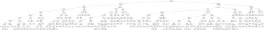
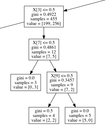
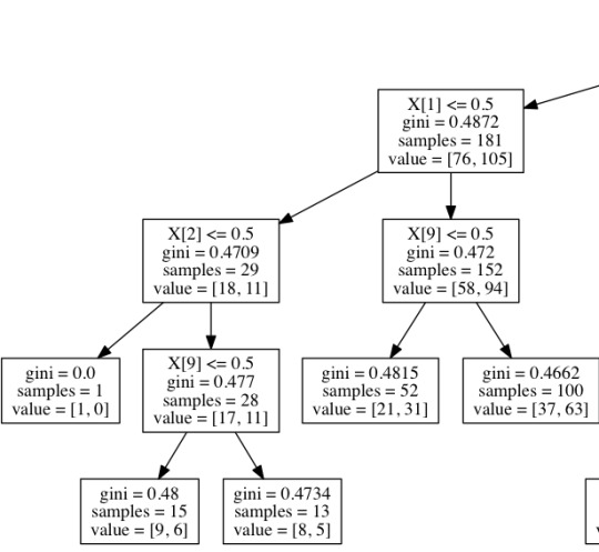
DECISION TREE

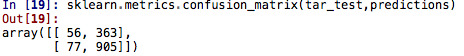
DATA DESCRIPTION

I performed the decision analysis with the National Longitudinal Study of Adolescent to Adult Health (Add Health) dataset. This survey has been conducted regularly since 1995, compiling data from a representative sample of American Adolescents in 7th to 12th grade. I’m testing the nonlinear relationships among the students performances (measured with a binary variable of pass/fail grades in various subjects) and the following explanatory variables: (race/ethnicity) Hispanic, White, Black, Native American and Asian; (parent’s education level) mother’s level of education and father’s level of education; (extracurricular activities) time spent watching tv, time spent in sports and whether the student has a job.

MODEL DESCRIPTION

Training sample: 2010 observations, 10 explanatory variables

Test sample: 1401 observations, 10 explanatory variables

The classification model’s yielded a 68 % accuracy. We saw that 55 observations were true negatives; 903 resulted on true positives (there are 903 observations correctly categorized as “passing” students); 68 were false negatives and 375 students were falsely classified as “passing”.

DECISION TREE VIZ

Here are some snapshots of what my decision tree looks like. 

CODE

@author: marindani11 """

from pandas import Series, DataFrame import pandas as pd import numpy as np import os import matplotlib.pylab as plt from sklearn.cross_validation import train_test_split from sklearn.tree import DecisionTreeClassifier from sklearn.metrics import classification_report import sklearn.metrics import pickle

#IMPORT DATA PREVIOUSLY CLEANED FOR THIS EXCERCISE with open('decisionTree.pickle', 'rb') as data:    dataset = pickle.load(data)

# SET RESPONSIVE AND EXPLANATORY VARIABLES predictors=dataset[['LATINOS', 'WHITE','BLACK','AMINDIAN','ASIAN','MOTHEREDU', 'FATHEREDU','TVTIME','SPORTSTIME','JOB']]

targets = dataset.GRADES

#INDICATE THE SIZE OF DATA SAMPLES FOR TRAINING AND TESTING "test_size indicates the % we want -  in this case 60% training sample, 40% test sample" pred_train, pred_test, tar_train, tar_test  =   train_test_split(predictors, targets, test_size=.4)

pred_train.shape pred_test.shape tar_train.shape tar_test.shape

#ONCE TRAINING AND TESTING DATASETS ARE CREATED WE CAN BUILD MODEL classifier=DecisionTreeClassifier() classifier=classifier.fit(pred_train,tar_train) "code to fit the model"

#PREDICT THE TEST VALUES predictions=classifier.predict(pred_test)

sklearn.metrics.confusion_matrix(tar_test,predictions) "to call in the confusion matrix function which we passed the target test sample to"

sklearn.metrics.accuracy_score(tar_test, predictions) "to learn how accurate the model classifies our dataset"

#VISUALIZE THE DECISION TREE from sklearn import tree from io import StringIO from IPython.display import Image out = StringIO() tree.export_graphviz(classifier, out_file=out) import pydotplus

#DATA VISUALIZATION - DECISIONTREE     graph=pydotplus.graph_from_dot_data(out.getvalue()) picname = "fig2.png" graph.write_png(picname) os.system("start"+ picname)

graph.savefig('/Users/marindani11/Desktop/Coursera/SPECIALIZATION/Python/decisiontree.png') plt.close(graph)

with open('/Users/marindani11/Desktop/Coursera/SPECIALIZATION/Python/picture_out1.png', 'wb') as f:    f.write(graph.create_png())

Image(graph.create_png())

[marindani11-blog]

MY DATA

SAMPLE

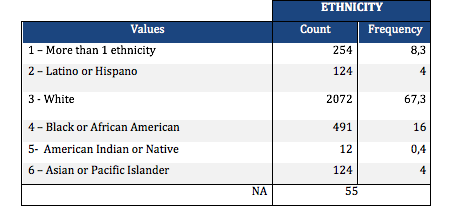
I have decided to work with the National Longitudinal Study of Adolescent to Adult Health (Add Health) dataset. This survey has been conducted regularly since 1995, compiling data from a representative sample of American Adolescents in 7th to 12th grade. The sample comprises 3077 students, which I’m studying at the individual level. The ethnic composition is predominantly White (n=2072, 67,3%), African American (n=491, 16%), More than 1 ethnicity (n=254, 8,3%), Latino (n= 124, 4%) and Asian (n= 124, 4%); and American Indian (n=12 , 0,4%). 

PROCEDURE 

This survey has been conducted regularly since 1995, compiling data from a representative sample of American Adolescents. 80 high schools and 52 middle schools from the US were selected. The original purpose of the research program was to help explain the causes of adolescent health and health behavior with special emphasis on the effects of multiple contexts of adolescent life. Incorporating sampling methods, this study is representative of US schools with respect to region of country, urbanicity, school size, school type, and ethnicity. The data was collected through In-school questionnaires, where students of participant schools will respond to questions in a 45- to 60-minute class period; and an In-home questionnaire. Following the in-school survey, student’s cohorts stratified by grade and sex were created. Then, 17 students from each cohort, randomly selected, were eligible for the in-home questionnaire. AddHealth has had multiple waves, the first wave starting in 1995 and the latest currently happening (2016-2018). 

VARIABLES 

I can study the correlation between the parent’s level of education and their children’s academic performance. Accordingly, I will associate the adolescent’s grades in different subjects (Add Health section 5) with how far it’s resident mother and father went in school (Add Health sections 14 & 15); while controlling for individualities (age, gender, race, etc.), household characteristics (income, size, composition) and other externalities, such as dedication (measured by the proxy: time spent studying). My explanatory variable is a categorical variable with 6 values. The response variable can either be study as a dummy variable (pass/fail) or a categorical variable with 4 values (grades A to D or lower).

[marindani11-blog]

TESTING MODERATION

Does ethnicity affects either the strength or the direction of the relation between the mother’s level of education (collapsed into 6 ordered categories) and their adolescent’s academic achievements (English grades (binary categorical variable – pass/fail))? 

 In order to accomplish this, we will need to study the Chi Square Value for each ethnicity group independently. For this assignment purpose I will look at the moderation for only 2 ethnic groups: Latinos (Ethnicity value = 1) and Whites (Ethnicity Value =2). 

 You can download the code here. 

LATINOS 

A Chi Square test of independence revealed that among “Latino” American adolescents (my sub-sample), the mother’s level of education (collapsed into 6 ordered categories) and grade results for English (binary categorical variable – pass/fail) were not significantly associated, X2 =1.58, p=0.90. 

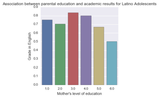
Mother’s schooling values: (1) Not graduated from high school, (2) High school or equivalent graduates, (3) Vocational school and professional training, (4) Not graduated from college, (5) Have a college degree and (6) Never attended school. 

WHITES 

A Chi Square test of independence revealed that among “White” American adolescents (my sub-sample), the mother’s level of education (collapsed into 6 ordered categories) and grade results for English (binary categorical variable – pass/fail) were significantly associated, X2 =61.3, p=1.55e-12. 

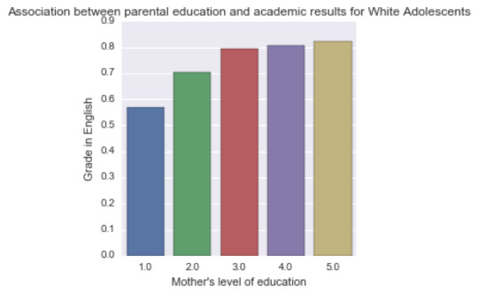
Post hoc comparisons of rates of English grades by pairs of maternal level of schooling categories revealed that, with an adjusted p value of 0.003 (0.05/15 pairwise comparisons) succeeding english grades were seen among those adolescents with mothers that had not graduated from high school, vocational training or with college educated mothers. The results of this test are visible in the code. 

Overall, the moderator (Ethnicity) does influence the relationship and the strenght between the explanatory and responsive variable

[marindani11-blog]

PEARSON CORRELATION

For this assignment I am analyzing the relationship between the time spent playing videogames a week, against the time spent working per week. The data I am using is the AddHealth survey, which compiles a representative sample of USA adolescents. 

 As you can see in my code (downloadable here), I started by cleaning the variables of interest and subsetting the data. I then created the following scatterplot:

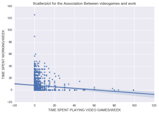
From this graph, we can already see that the relationship is negative. Most of the population is distributed around 0 to 20 hours of video gaming per week. 

Next, we need to analyze the relation with a Pearson Correlation Coefficient:

CODE: print (scipy.stats.pearsonr(data_clean['VIDEOGAMES'], data_clean['WORK'])) 

RESULTS: association between videogames and work (-0.088785527753423077, 0.00041559081499293075) 

The r shows a negative weak (close to 0), yet significant (p value < 0.05) relation between the two variables. If we look at the r2 (=0.008) , we can say that knowing the variability of adolescent spent playing video games, we can predict 0.8% of the time they would spent working.

[marindani11-blog]

CHI SQUARE TEST OF INDEPENDENCE

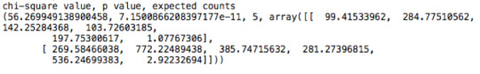
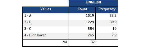
A Chi Square test of independence revealed that among American adolescents (my sample), the mother’s level of education (collapsed into 6 ordered categories) and grade results for English (binary categorical variable – pass/fail) were significantly associated, X2 =56.27, p=7.15e-11.

CODE:  x2test= scipy.stats.chi2_contingency(obscounts)

RESULT:

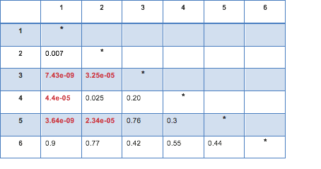
Post hoc comparisons of rates of English grades by pairs of maternal level of schooling categories revealed that, with an adjusted p value of 0.003 (0.05/15 pairwise comparisons) succeeding english grades were seen among those adolescents with mothers that had vocational training or with college educated mothers. The following table represents those results:

Mother’s schooling values: (1) Not graduated from high school, (2) High school or equivalent graduates, (3) Vocational school and professional training, (4) Not graduated from college, (5) Have a college degree and (6) Never attended school.

You can see the full code (in python) here

[marindani11-blog]

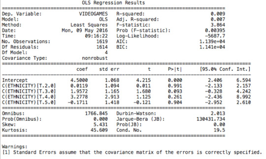
ANOVA F TEST

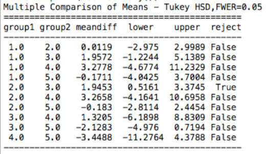
ANOVA revealed that among weekly video game players (my sample = 1619 American adolescents), ethnicity (collapsed into 5 ordered categories, which is the categorical explanatory variable) and the number of hours per week spent playing video games (quantitative response) were significantly associated, F (4, 1619)= 3.864, p= 0.00395. Post hoc comparisons of mean number of weekly hours spent playing video games by ethnicity revealed that white adolescents reported significantly more weekly hours spent playing video games compared to black adolescents. All other comparisons were statistically similar.

Anova F Test:  

model1=smf.ols(formula='VIDEOGAMES~ C(ETHNICITY)',data=sub1).fit()  

print (model1.summary())

Post Hoc Tukey HSD Test 

mc1 = multi.MultiComparison(sub1['VIDEOGAMES'], sub1['ETHNICITY']) 

res1 = mc1.tukeyhsd()

print(res1.summary())

The complete code can be downloaded here

[marindani11-blog]

VISUALIZING DATA

For my research question, I am exploring the relation between student’s grades with their parent’s level of schooling. Both explanatory and dependent variables are categorical in my dataset.

I began by creating descriptive graphs for each variable. Since last week I constructed a subset of my data, I am sure I will not encounter any missing data or unwanted values. The following 2 graphs are extracted from my study (you can see all the variables and corresponding graphs in my code):

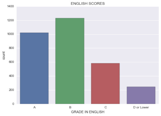
1) English score: This variable has 4 values representing the grade each student (3077 observations) got in English. Its distribution is a unimodal distribution, with its node being “Grade B”. Since it’s a categorical variable, I can’t calculate the standard deviation. I do know, however, the frequency of getting the top value (“B”) is 1229. 

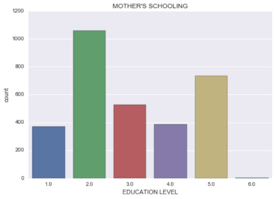
2) Mother’s education level: – (1) Not graduated from high school, (2) High school or equivalent graduates, (3) Vocational school and professional training, (4) Not graduated from college, (5) Have a college degree and (6) Never attended school. It has a non-symmetric distribution with 2 nodes. The first node and most frequent value (1057 observations) is “High school graduates”, and the second node is “College graduates”.

Next, I collapsed my responsive variables into dummy variables to create a bivariate graph C to C. The grades for the different subjects were transformed into dummy variables representing pass/fail scores. Here is an example of the outcome (you can see all the other bivariate graphs in the code:  

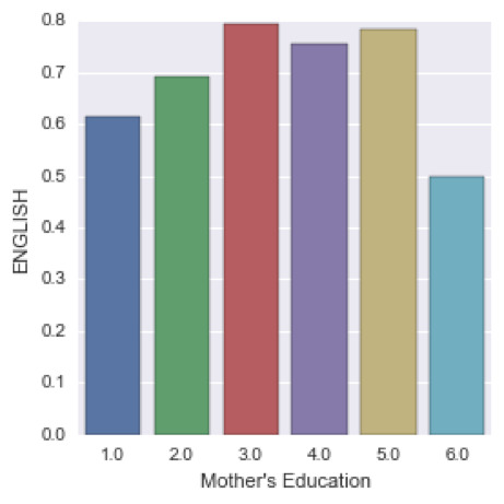
We can see that the highest percentage of students passing English have mother’s with a vocational training, followed by students with college graduate mothers. The lower probability of passing english corresponds to adolescents with uneducated mothers. 

The results from this first visual analysis is in sync with my preliminary hypothesis. 

[marindani11-blog]

MAKING DATA MANAGEMENT DECISIONS

My first data management decision was to code out values that are not informative for my research purpose. Concerning the adolescent’s grades in english, math, science and history, I have excluded all the irrelevant values such as “don’t know”, “refused” or “legitimate skip”. I also did a similar procedure for the variables relevant to parent’s education. After validating the code (the missing values in the new variable coincide with the sum of irrelevant statements), I found consistent results with the previous week assignment.

Next, I used the same approach to recode the parents’ level of education. Originally, the variable had 10 different values. I decided to group the into the following categories: 

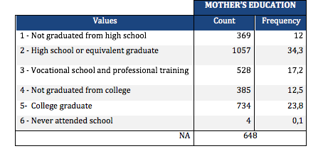
After checking the code was correct, I found that 34,3% (highest frequency) of mothers had graduated from high school, 23,8% had graduated from college, while only 0,1% had never attended high school. The father’s level of schooling has a very similar distribution.

Lastly, I created a secondary variable aggregating the different adolescent’s ethnicities into one. I can see that 2072 adolescent’s in my sample are white, being the predominant ethnicity. The least represented ethnicity is American Indian or Native with only 0,4%.

You can see the complete analysis and program code (in python) here

Note: I know my code will be smoother using some loops; I’m looking into it.

[marindani11-blog]

EXPLORATORY DATA ANALYSIS WITH PYTHON

In order to measure the correlation I am interested in, how parent’s level of education influence their children’s academic performance, I will start by summarizing the following variables: adolescents grades in english, math, science and history; and the schooling level for their respective mothers and fathers (or equivalent). To fit my purpose, I am subsetting the data excluding missing values and other irrelevant values such as “don’t know”, “refused” or “legitimate skip”. The population I’m now studying is 3099 students.

From the univariate analysis, I’ve found that the students had better grades for history and science, with a frequency of getting an “A” of 39,6 % and 36,7% respectively. In english and math, however, the weight is placed on a “B” score.Regarding the mothers level of education, 30,6% (highest frequency) of mothers had graduated from high school, 23,9% had graduated from college, while only 0,2% had never attended high school. The fathers level of schooling has a very similar distribution: 29,8% had finished high school, 22,9% had graduated from college and only 0,3% never attended high school.

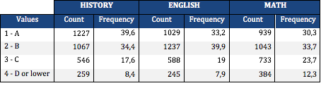
The distributions for the 3 of the before mentioned variables are described in the table below:

You can see the complete analysis and program code (in python) here

[marindani11-blog]

INTERGENERATIONAL EFFECTS OF EDUCATION

For this assignment, I have decided to work with the National Longitudinal Study of Adolescent to Adult Health (Add Health) dataset. Since the data includes the adolescent’s family background, I can study the correlation between the parent’s level of education and their children’s academic performance. Accordingly, I will associate the adolescent’s grades (Add Health section 5) with how far it’s resident mother and father went in school (Add Health sections 14 & 15); while controlling for individualities (age, gender, race, etc.), household characteristics (income, size, composition) and other externalities.

I am expecting to find a positive and significant result in my research since the existing literature proves that parental, and the household environment, influence the behavior of children and adolescents. Alan B. Krueger (2004) demonstrates that financial constraints significantly impacts school attainment. Thus, children who are brought up in less favorable conditions are more likely to obtain less education (James J. Heckman and Dimitry Masterov 2004). Aside from the positive externalities associated with highly educated parents (such as income level), Pedro Carneiro and Heckman (2003) suggest that said education levels contribute to other family fixed effects that have a much more positive role on the offspring choices.

More interestingly, I’ll like to identify the channels through which the correlation is stronger. Are the spillover effects greater when they come from the mother or the father? The literature seems to show that maternal education has a larger impact than paternal education, since generally the mothers are the main care providers within the household. Economists showed that mothers’ level of education shapes their children’s health (Behrman and Deolalikar 1988). It does so through three possible channels: their acquisition of health knowledge, their literacy and numeracy skills and finally through attitudes they developed (Glewwe 1999). In return, children’s health determines their school attendance (Miguel and Kremer 2004).