mechanicalengineeringblog - Tumblr blog

[mechanicalengineeringblog]

Fire Hazard Regulations and How Wastewater Facilities Should Deal With Them

Although rare, fire-related accidents do occur in wastewater treatment and collection facilities. Chlorine, ammonia, methane and hydrogen sulfide can quickly build up in confined spaces. Volatile conditions in hazardous locations can lead to catastrophe.

The National Fire Prevention Association (NFPA) 820 standard dictates how to address fire and explosion hazards in wastewater facilities. It offers safeguards against the ignition of combustible gases, health concerns and accumulation of airborne contaminants. It applies to new construction, and additions or modifications to existing facilities.

Owners, architects and general contractors are advised to pay close attention to this standard. While the chances of an incident may appear small, the consequences are dire: Lawsuits, OSHA inspections, loss of business and PR fallout. From a business perspective, too, NFPA 820 cannot be ignored. Owners are now starting to include it in RFPs. Those failing to include its provisions in designs are likely to fail in bids.

However, compliance can pose problems. The complex nature of airflows below ground, the flow characteristics of sludge, and particulate concentrations in enclosed areas are only a few of the challenges. The standard calls for air changes as the solution to contaminant build up. The number of air changes is adjusted based on the type of particulate, the presence of inflammable gases, enclosed spaces and other factors.

NFPA 820 demands anywhere from six to 12 changes of air per hour per room. The owner is asked to provide proof the standard has been met. Traditionally, engineers calculated room volume and added enough airflow to obtain twelve times that amount and deliver moving air at the desired level. Unfortunately, dead zones remain. There is no way to verify that all particulate has been removed. Tracer gases are another technique. While sometimes useful for existing facilities, it is impossible to apply for spaces that do not yet exist and it is more time and money consuming than other techniques.

But there is a way to ensure compliance with NFPA 820 and prove adherence to the rigors of its many clauses. Maya HTT has the expertise to apply Computational Fluid Dynamics (CFD) to wastewater collection, treatment facilities, high-rises, tunnels, warehouses, data center and more.

How does it work? The 3D geometry of the facility is taken from the Building Information Model (BIM). When combining with simulation and modeling software, a CFD analysis provides an easy, affordable and effective way to safeguard spaces. It accurately assesses the concentration of pollutants and contaminants. Its simulations highlight airflow velocity, pressure, direction, temperature, concentration and more. Dead spots become immediately apparent, enabling those designing and building spaces to take remedial action and validate those changes with a time and cost effective approach.

At times, more air diffusers will be required, or the direction or volume of airflow will have to be adjusted. But in other instances, fewer air movers may be necessary. Only precise CFD-based modeling providers owners, architects, designs and builders with the peace of mind that hazard protection has been successfully instituted.

[mechanicalengineeringblog]

Industrial AI Applications – How Time Series and Sensor Data Improve Processes

(This article was written by TechEmergence Research and originally appeared on: https://www.techemergence.com/industrial-ai-applications-time-series-sensor-data-improve-processes/)

Over the past decade the industrial sector has seen major advancements in automation and robotics applications. Automation in both continuous process and discrete manufacturing, as well as the use of robots for repetitive tasks are both relatively standard in most large manufacturing operations (this is especially true in industries like automotive and electronics).

One useful byproduct of this increased adoption has been that industrial spaces have become data rich environments. Automation has inherently required the installation of sensors and communication networks which can both double as data collection points for sensor or telemetry data.

According to Remi Duquette from Maya Heat Transfer Technologies (Maya HTT), an engineering products and services provider, huge industrial data volumes don’t necessarily lead to insight:

“Industrial sectors over the last two decades have become very data rich in collecting telemetry data for production purposes… but this data is what I call ‘wisdom-poor’… there is certainly lots of data, but little has been done to put it into productive business use… now with AI and machine learning in general we see huge impacts for leveraging that data to help increase throughput and reduce defects.”

Remi’s work at Maya HTT involves leveraging artificial intelligence to make valuable use of otherwise messy industrial data. From preventing downtime to reducing unplanned maintenance to reducing manufacturing error – he believes that machine learning can be leveraged to detect patterns and refine processes beyond what was possible with previous statistical-based software approaches and analytics systems.

During our interview, he explored a number of use-cases that Maya HTT is currently working on – each of which highlights a different kind of value that AI can bring to an existing industrial process.

This point is reiterated in an important slide from one of his recent presentations at the OsiSoft PIWorld Conference in San Francisco:

Use Case: Discrete Manufacturing

Increasing throughputs and reducing turnaround times are some of the biggest business challenges faced by the manufacturing sector today – irrespective of industry.

One interesting trend here was that individual machine optimization was the most common form of early engagement with AI for most manufacturers – and much more value can be gleaned from simultaneously optimizing the combined efficiencies of all the machines in a manufacturing line.

“There has been little that has been done to really help that industry to go beyond automation and statistical-based procedures, or optimizing individual machines.

What we find in our AI engagements is that – at the individual machine level – there is little that can be done, as it’s been fairly optimized… if we look at where AI can help significantly, it’s at looking at the production chain as a whole or combining different type of data to further optimize a single machine or a few machines together.”

In a typical discrete manufacturing environment today, we would likely find that there are over ten manufacturing stages and that data is collected at each stage from a plethora of devices. Remi explains that in such a scenario AI can today track correlations between many machines and identify patterns in the industrial data which can potentially lead to overall improved efficiency.

He adds some color here with a real-life example from one of Maya HTT’s clients. He elaborates that for one particular discrete manufacturer’s industrial process which faced high rejection rates, Maya HTT collected around 20,000 real-time telemetry variables and by analysing the data along with manufacturing logs and other non real-time production data, the AI platform was able to find what led to the high rejection rates.

“A discrete manufacturing process with over 10 manufacturing stages – each collecting tons of data. Yet towards the end of the process there were still high rejection rates… In this case we applied AI to look at various processes throughout this ‘food chain’.

There were 20,000 real-time telemetry variables collected, and by correlating them and combining them with production data, the AI was able to learn which combinations and variance led to the rejection rate. In this particular case the AI was able to remove over 70% of the rejection issues.”

This particular AI solution was able to quickly recognize faulty pieces so the machine operators could remove them from the process thereby reducing the work that the quality assurance team had to handle and leading to saved material and less real work hours spent detecting or correcting faulty pieces.

What this means in real business terms is that the manufacturer used fewer raw materials, had a lot less rework hours, which essentially translated to saving of half a million dollars per production line per year. “We estimated a savings of over $500,000 per year in this particular case”, said Remi.

Use Case: Fleet Management

Another such use-case that Remi explored was in fleet management or freight operations in the logistics sector where maintaining high fuel efficiency for vehicles like trucks or ships is essential for cost-savings in the long run.

Remi explains that AI can enable ‘real-time’ fleet management which would otherwise be difficult to achieve with plain automation software. Various patterns identified by AI from data, like weather or temperature conditions, operational usage, mileage, etc can potentially be used to pick out anomalies and recommend what the best route or speed would be in order to operate at the highest efficiency levels.

Remi agreed that no matter the mode of transportation used (trucks or ships, for example), some of the more common emerging use-cases for AI in logistics are around overall fuel consumption analysis for fleets.

“When you have a large fleet, it’s possible to mitigate a lot of loss by finding refinements in fuel use.”  In cases of very large fleets, AI can simulate and potentially mitigate huge loss exposure by reducing fuel consumption for the fleet.

Use Case: Engineering Simulation

The last use-case that Remi touched on was 3D engineering simulations for design in the field of computational fluid dynamics.

Traditional simulation software can be fed input criteria like flow rates of fluids and can generate a 3D simulation which usually takes around 15 minutes to be rendered and involves a long, iterative, and often manual process.

Maya HTT’s team claims that it was able to deliver an AI tool for this situation resulting in getting simulation results time falling to less than 1 second. Maya HTT claims that this improvement of over 900x in efficiency gains (from 15 minutes to 1 second) during the design process enabled design teams to explore far more design variants than previously possible.

Phases of Implementation for Industrial AI

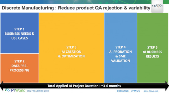
When asked about what business leaders in the manufacturing sector interested in adopting AI would need to do, Remi outlines a 5 step approach used at Maya HTT:

The first step would be a business assessment to make sure any target AI project will eventually lead to significant business impact.

Next businesses would need to understand data source access and manipulations that may be needed in order to train and configure the AI platform. This may also involve restructuring the way data is collected in order to enhance compatibility.

The actual creation and optimization of an AI application.

Training and conclusions from AI need to be properly explained and understood. The operational AI agent is put to work and final tweaks are made to improve accuracy to desired levels.  

Delivery and measurement of tangible business results from the AI solution.

In almost all sectors we cover, data preprocessing is an underappreciated (and often complex) part of an AI application process – and it seems evident that in the industrial sector, the challenges in this step could be significant.

A Look to the Future

Remi believes that for the time being, industrial AI applications are safely in the realm of augmenting worker’s skills as opposed to wholly replacing jobs:

“At least for the short-medium timeframe… we augment people on the shop floor in order to increase throughput and production rates.”

He also stated that the longer-term implications of AI in heavy industry involve more complete automation – situations where machines not only collect and find patterns in the data, but take direct action from those found patterns. For example:

A manufacturing line might detect tell-tale signs of error in a given product on the line (possibly from a visual analysis of the item, or from other information such as temperature and vibration as it moves through the manufacturing process), and remove that product from the line – possibly for human examination, or simply to recycle or throw out the faulty item.

A fleet management system might detect a truck with unusual telemetry data coming from its breaks, and automatically prompt the driver to pull into the nearest repair shop on the way to the truck’s destination – prompting the driver with an exact set of questions for the diagnosing mechanics.

He mentions that these further developments towards autonomous AI action will involve much more development in the core technologies involved in industrial AI, and a greater period of time to flesh out the applications and train AI systems on huge sets of data over time.

Many industrial AI applications are still somewhat new and bespoke. This is due partially to the unique nature of manufacturing plants or fleets of vehicles (no two are the same), but it’s also due to the fact that AI hasn’t been applied in the domain of manufacturing or heavy industry for as long as it has been in the domains of marketing or finance.

As the field matures and the processes for using data and delivering specific results become more established, AI systems will be able to expand their function from merely detecting and “flagging” anomalies (and possibly suggesting next steps), to fully taking next steps autonomously when a specific degree of certainty has been achieved.

About Maya HTT

Maya HTT is a leading developer of simulation CAE and DCIM software. The company provides training and digital product development, analysis, testing services, as well as IIoT, real-time telemetry system integrations, and applied AI services and solutions.

Maya HTT are a team of specialized engineering professionals offering advanced services and products for the engineering and datacenter world. As a Platinum level VAR and Siemens PLM development partner and OSIsoft OEM and PI System Integration partner, Maya HTT aims to deliver total end-to-end solutions to its clients.

The company is also a provider of specialized engineering services such as Advanced PLM Training, Specialized Engineering Consulting for Thermal, Flow and Structural projects as well as Software Development with extensive experience implementing NX Customization projects.

[mechanicalengineeringblog]

Crypto Farms  a Lot of Hot Air?

Crypto farms are big news these days. Some question the value that can be gained from cryptocurrencies such as Bitcoin and Ethereum. A few go as far as to say it is a whole lot of hot air.

In one sense they are correct. Crypto farmers cram massive amounts of computing density into tiny spaces. These banks of servers generate hot air in large quantities the successful ones transform it into a lucrative revenue source.

What determines success? How well a space is laid out to pack as much computing muscle into one place while facilitating the inflow of cold air and the removal of hot air. Unfortunately, there is no single room layout or design to help crypto farmers achieve this.

Traditional data centers were often subjected to careful design and planning all the way down to the construction of a new facility. Best practices improved over the years about the use of redundant computers and electrical systems, raised floors, hot aisles and cold aisles, backup generators, batteries, and the deployment of air handling units (AHUs). This resulted in some wonderfully efficient data centers. But there was one big problem: Cost. These facilities were expensive to equip and run.

Crypto farmers don’t have the budget, the margins or the time to take the traditional route. They typically use whatever space is available, cram in as many multi-core servers and Graphics Processing Units (GPUs) as possible, and get to work mining cryptocurrency. Some use a room in a house, a small office space or an unused basement. Others utilize large warehouses where the hot air can dissipate easily. More than a few find containers an ideal place to stack hundreds of servers in their crypto farms.

Most of these spaces, however, soon face challenges with regards to overheating, rising electricity costs and low efficiency. It’s all very well to pile banks of servers into a small office or container. But if the expelled air can’t escape rapidly, the equipment will eventually shut down.

The best way to solve these issues is simulation. It is possible to simulate room conditions to optimize the position of servers and determine how best to set up the airflow. As every crypto farm is unique, this has to be done on an individual basis.

Some may argue that there is no time for lengthy design, simulation and optimization efforts. The crypto mining rush is on and there is no time to lose. However, simulation is fast and has a rapid return on investment. Those in too much of a hurry to simulate their farms may regret it when their equipment overheats. In some cases, they spend twice as much fixing the problems caused by poor room layout.

A simple simulation can rapidly determine the optimum amount of computing density for a specific square footage. It calculates the temperature, the air velocity and the interchange of hot and cold air in the facility. A heat map is produced which highlights equipment hot spots that are likely to result in a server meltdown. This is accompanied with recommendations on how to modify the room configuration to optimize crypto mining efficiency, performance and cost.

In this fiercely competitive field, time is of the essence. But those willing to spend the time on simulation, find their mining efforts enhanced, their equipment no longer subject to sudden shutdowns and their profitability rising. By simulating their spaces, they see where hot air may build up, how best to channel it away from hotspots, and how to import cold air from outside to cool the environment. Done right, this can sometimes be achieved without the need to purchase AHUs, coolers, large fans or other equipment.

Maya HTT helps crypto miners and engineering firms to optimize cooling efficiency and compute density. These simulations validate room design during construction without the need for delay. They can also take advantage of free cooling and natural ventilation to eliminate some of the biggest crypto farming expenses.

Maya HTT has worked with over one hundred data centers and crypto farmer sites. Maya HTT’s expertise in Computational Fluid Dynamics and simulation helped them establish highly productive, efficient and cost-effective computing spaces.

Contact Maya HTT today to validate and optimize your crypto farm design: https://www.mayahtt.com/about-us/contact-us

Author: Olivier Allard

[mechanicalengineeringblog]

Validating a Simplified FEM using Simcenter FE Model Update

Quick Overview

It is often required to create lightweight, simplified versions of large FEMs in order to reduce solution time or post-processing effort. A common simplification technique that can be used with relatively slender parts is midsurfacing. Whereas plate theory can accurately predict the stiffness of each part, there can be uncertainty at the structural connections  be they welded, bonded or fastened- due to the idealization of the part thickness and the creation of non-manifold joints.

Simcenter FE Model Correlation and FE Model Update allow you to compare the modal properties of fine and simplified FEMs, as well as to automatically update the simplified FEM to minimize the differences. In this example, we’ll take a relatively large FEM of a cone with 2 welded flanges as reference, and update a simplified, midsurfaced version of the FEM so that the modal frequencies agree well. The simplified model will provide the work solution. We’ll also create the 2 FEMs.

Core content

Create Reference FEM

Starting with the CAD geometry, we first create the larger reference FEM and SIM, using NX Nastran as solver:

Set the Solution Type to SOL 103 Real Eigenvalues

Create a parabolic tetrahedral mesh of the part using the default size computed by Simcenter:

As material, select Aluminum_6061 from the Simcenter materials library

Make the SIM the work part, select the 2 bottom faces of the flanges to define fixed constraints:

Solve the normal modes Solution. 10 modes are computed, the first being at 1318 Hz.

Create Work FEM

Go back to the part file in the modeling application.  Create a new NX Nastran FEM and SIM, and set the Solution Type to SOL 200 Model Update

Using the Simulation File View, navigate to the idealized part.

Create an associative copy of the CAD part using WAVE linking. Do not hide the original part.

Click Midsurface by Face Pairs

Select the solid body and click Automatically Create Face Pairs. The midsurfaced part looks like this

Create 4 datum planes, one on each vertical face of the 2 flanges

Divide the cone sheet body faces using the datum planes to create 4 new faces around the flange joints. The meshes on these faces will be assigned a material property which will be used by FE Model Update.

Return to the fem. Hide the original polygon geometry, keeping the newly created sheet bodies. Use Merge Faces to get rid of the unneeded divisions on the top of the cone

Use Automatic Stitch Edge to merge the coincident edges of the flanges and the cone. Create 3 different 2D meshes and place them in the following collectors:

1- A collector for the general cone section

2- A collector for the joint section which will be optimized.

3- Finally, a collector for the flanges

Shift-Select the 3 meshes in the sim navigator, Edit Mesh Associated Data,

And set the thickness source to Midsurface. Select the general cone section collector, Edit the PSHELL1 property and select Aluminum_6061 as material. Select the flange collector, and assign PSHELL1 to it. Then select the joint section collector, Edit the PSHELL2 property, and assign to it a copy of Aluminum_6061 which you rename OPTIM.

Go the SIM.

Create a new Material Design Variable

Select OPTIM and its field E (Modulus) as design variable.

Create fixed constraints at the base of the 2 flanges

Edit the solution. In the Bulk Data tab, Create Design Variables

Add to the active list the variable you just created. Set the Model Reduction method to Modal, and create a New DOF set

Select all the nodes in the FEM, and check DOFs 1, 2 and 3

Solve the solution. Note the first mode is at 1053 Hz.

Correlate Work and Reference Models

In the Correlation tab, create a New Analysis Reference Solution.

Select the .op2 file from the SOL 103 solution using the reference FEM.

In the Correlation tab, create a New Correlation and select the Work and Reference solutions

Select the Mode Pairs node in the SIM navigator, open the Correlation Details View, and notice there are significant frequency errors between both models. However the mode shapes correlate very well, as indicated by the high MAC value for each mode pair.

Model Update

We will now optimize the work model to improve the correlation with the reference model. Create a New Model Update

Select the same solutions as for the Correlation. Notice the single design variable is displayed with an initial, normalized value of 1

In the Model Update group of the Correlation tab, click Optimize

Since we’re not concerned about limiting the change in the design variable, set the Overall Design Variable Weight to 1%

The optimization ends with the design variable reaching its default upper limit of 2:

Comparing Current and Initial frequency errors, we notice an improvement, which is not as significant as expected because of the limit on the design variable.

We can edit the design variable’s Upper Bound and set it to 4

After optimization, we notice a much better correlation

The JOINT design variable’s normalized value is now 3.

This means the Young’s Modulus of the OPTIM material has tripled, which is a substantial change. Since SOL 200 Model Update Solution returns first-order sensitivities which are valid for small changes, the solution needs to be updated. In the Model Update group of the Correlation tab, click Update Finite Element Model. This command automatically updates the material and physical properties in the FEM.

The new value of E for material OPTIM is 2.07 X108 kPa, from the original value of 6.98 X107 kPa

Re-solve the SOL 200 Model Update solution, Reset the Design Variable to 1 using the Reset command and Refresh the Model Update. We notice that the frequency errors are different than after the previous optimization, this is because of the linear sensitivities:

Optimize once again

Let’s now Update the FEM. The new value of E is 4.14 X108 kPa.

Re-solve the SOL 200 Solution and Refresh the Model Update. The frequency error for the first mode pair is less than 1%, it was originally around 20%. Side-by-side mode shape displays complement the Correlation Details View.

All MAC values are above 0.96. The largest frequency difference is for mode 9, 7.7%. It was originally around 15%

By changing the optimizer settings, it’s possible to reduce the maximum error for all 10 modes to less than 5%, however this results in an increase in the error for mode 1, which may be the most important mode due to its effective mass.  The maximum error can also be reduced by further splitting the faces of the work model and creating more design variables.

Summary

We have validated a simplified FEM that contains 706 nodes (around 3500 dofs) against a finer reference FEM containing 10587 nodes (around 31500 dofs  10 X more than the simplified FEM). In reality the reference FEM should be even finer, such that there are 2 layers of elements through the thickness. The first mode correlates with a MAC of 1 and a frequency difference below 1%. Other modes also show excellent shape correlation, with a maximum frequency error around 8% for the ninth mode.

[mechanicalengineeringblog]

Correlating Simulation & Modal Test Results with Simcenter 3D

Quick Overview

A powerful way of reducing design conservatism is to validate the finite element model used to simulate its performance. Comparing the simulation model’s natural frequencies and mode shapes with those acquired in test generates confidence in the model’s ability to represent the as-built structure. This in turn allows analysts to reduce the safety factors used to compute structural margins of safety. Simcenter 3D FE Model Correlation supports both test and simulation engineers who wish to perform such a comparison, efficiently providing both visual and quantitative feedback. 

Background

The Modal Assurance Criterion (MAC) is a parameter indicating the degree of consistency between a mode shape from test and another one from simulation. This parameter is a scalar value between 0 and 1: A MAC value near 1 indicates a high degree of correlation or consistency between two mode shapes.

Suppose {ΨA} and {ΨX} are two mode shapes that you want to compare: Their MAC is expressed as follows:

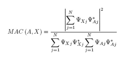
Where:

N is the number of common simulation and test mode shape components

The superscript * indicates the complex conjugate value.

There are LA x LX MAC numbers for given mode shape matrices [ΨA] and [ΨX], where LA is the number of mode shapes in [ΨA] and LX is the number of mode shapes in [ΨX]. These are presented in matrix format:

Problem Definition

We wish to compare the natural frequencies and mode shapes of an aircraft engine nacelle finite element model with the equivalent data acquired during a modal test of the actual structure:

The model and test article both represent half the nacelle.

1. Normal Modes Solution

First we create an NX Nastran normal modes solution, requesting the first 20 free-free (unconstrained) modes of the FEM. The first 6 modes describe rigid body motion, in which the structure moves without any internal strain. The next 14 modes are elastic modes, which are the ones we are interested in correlating.

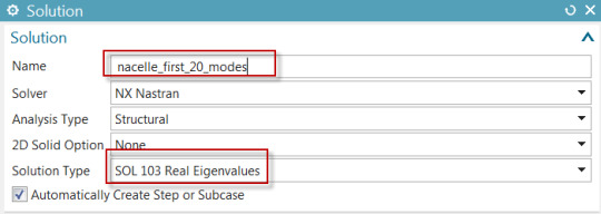
In the simulation navigator, select the top-most sim node and right-click New Solution

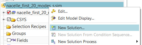
The Solution dialog pops up. Enter a Name and as Solution Type, select Sol 103 Real Eigenvalues from the list

In the Case Control tab of the Solution dialog, next to Lanczos data click Create Modeling Object

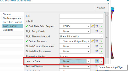
  In the Real Eigenvalues  Lanczos dialog, enter 20 as the Number of Desired Modes. Click OK twice.

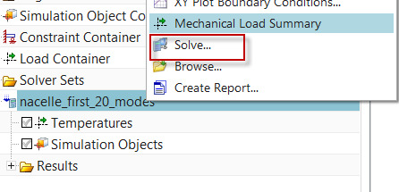
In the sim navigator, select the solution, right-click, Solve

After the solution is complete, the mode shapes can be displayed from the post navigator.

2. Import Test Geometry and Results

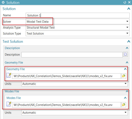
In the Correlation tab of the Simcenter 3D ribbon, click New Test Reference Solution

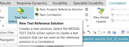
Set the Solution Type to Modal Test Data, and then select a Geometry File which contains the test geometry (test sensors, coordinate systems and traces) as well as a Modes File containing the test mode shapes and natural frequencies. In this case, the same file contains both the geometry and the mode shapes.

Click OK.  There are now 2 solutions in the sim file.

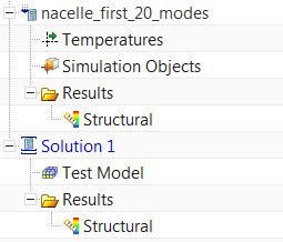
Since Solution 1 is active and points to imported geometry, the fem is now displayed as monotonic grey.

3. Align the Test Model

In the sim navigator, under Solution 1, select the Test Model node, and right-click Show Model.

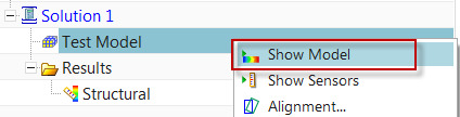
You can also click Show Sensors, to see the individual sensors as triads.

It is clear that the test model and the FEM do not share the same global coordinate system. The test model will have to be aligned with the FEM in order for correlation to be possible.

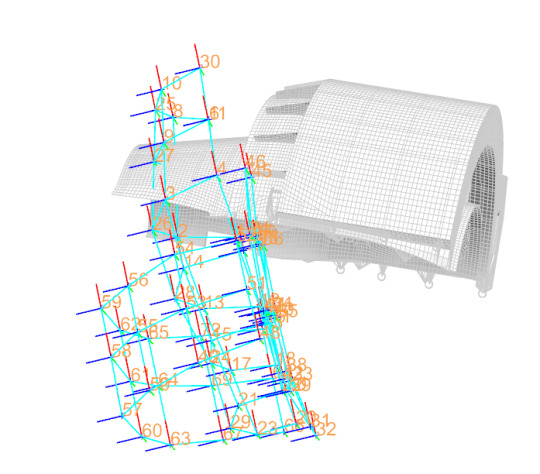
In the sim navigator, under Solution 1, select the Test Model node, and right-click Alignment. The Alignment Control dialog will appear, allowing you to choose 3 test nodes and the equivalent 3 nodes in the FEM. Checking on Preview allows you to see the cumulative effect of the pairs you have selected.

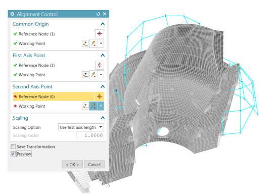
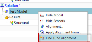
You may need to repeat this step if it is not clear which test sensors correspond to which nodes. After you have successfully performed the alignment, you may select Fine Tune Alignment to further nudge the test model by specifying discrete translations and rotations.

4. Create a Correlation

In the Correlation tab of the Simcenter 3D ribbon, click New Correlation

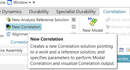
The Correlation dialog appears. Select test Solution 1 as the Reference Solution, and your normal modes solution as the Work Solution

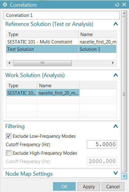
By default, low-frequency (rigid-body) modes are filtered out. In the Node Map Settings group, enter 75 mm as the matching tolerance between the test sensors and the FEM nodes.  Click OK.

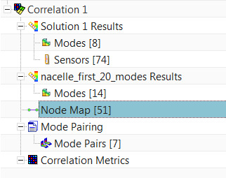
Based on the alignment that was performed, and the tolerance entered in the last step, Simcenter FE Model Correlation was able to map 51 sensors to the FE model nodes, based on proximity. If you repeat the alignment and choose different alignment node pairs, you will see a different number of paired nodes in brackets. The test and analysis mode shapes will be interrogated at these 51 locations to determine the MAC.

Next, select the Mode Pairing node under Correlation 1, right-click Edit. The default mode pairing criterion is MAC with a minimum value of 0.7: This means that test and analysis modes having the greatest MAC value above 0.7 will be paired, others will not be paired. For example, work (analysis) mode 12 is not paired to any test mode.

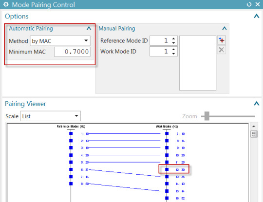
Other pairing methods can be selected.

Next, select the Mode Pairs (n) node under the Mode Pairing node and click the Correlation Details View bar

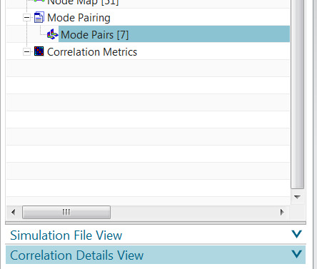
This pops up the Correlation Details View, which shows the test (reference) and analysis (work) frequencies, percent frequency error and MAC, for each mode pair.

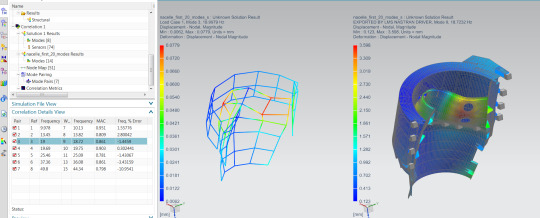
Select any mode pair row in the table, right-click Side-by-Side Animation:

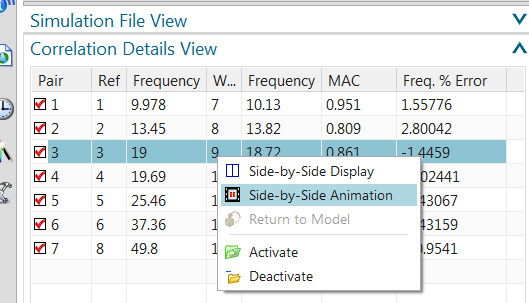
This will bring up a synchronized 2-view layout, showing the test and analysis mode shape animation

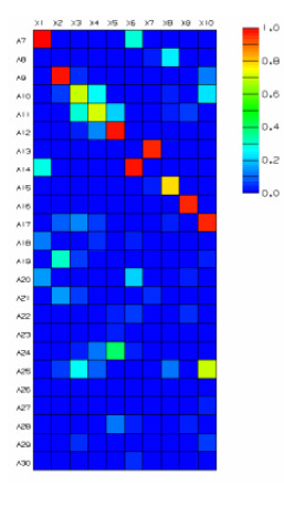
Select the Correlation Metrics node under Correlation 1, right-click Correlate. In the Correlate dialog, click Show Results Heat Map

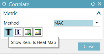
The heat map display shows the MAC matrix

In the Correlate dialog, click Show Results Spreadsheet

SC FE Model Correlation will send the MAC matrix to an Excel spreadsheet.

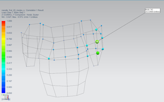
Select the Correlation Metrics node under Correlation 1, right-click Generate 1-COMAC Results.

This will show sensors at which the individual MAC components are poorest.

[mechanicalengineeringblog]

How to map flow forces to a structural analysis in Simcenter

Quick Overview

Simcenter offers a dedicated application to map steady state or transient flow results onto a target model, typically an independent structural model from the same geometry but with a different mesh. For example, one could be interested in the stress and distortion analysis of a canopy due to wind forces.

The target FEM must use the same global coordinate system as the source FEM, and both models should be geometrically congruent. However, they need not share the same mesh. Results are mapped from the selected solution on the source model, to a solution on the target model, based on proximity and with optional zone associations. The output of the mapping solution can then be used by the target solution.

In what follows, we describe how to create an NX Nastran structural analysis using forces that are mapped from a Simcenter Thermal/Flow analysis.

Workflow overview

The main steps are:

Create a part file containing the structure and air volume.

Create a Simcenter Thermal/Flow fem file with only the air volume meshed.

Create a new Simulation containing a Thermal/Flow Solution with Flow Analysis.

Run the Thermal/Flow Solution.

Back to the part file; create a NX Nastran fem file of the structure.

Create a new Simulation containing a Thermal/Flow Solution with Mapping Analysis.

Specify the mapping target area then Solve.

Assign the structural boundary conditions and solve the structural analysis.

For more information, see Simcenter Thermal/Flow, Electronic Systems Cooling, and Space Systems Thermal documentation.

Create the Thermal/Flow Simulation

1.     Create the part

We begin by creating the part file, as shown in Figure 1. This represents a simple tubular structure submitted to lateral winds.

Figure 1: Part file containing both structure and fluid volume

2.     Create the Thermal/Flow FEM

Next, create the fem file. In the “Edit FEM” window, make sure to choose Simcenter Thermal/Flow (Flow) as the “Solver Environment”, as shown in Figure 2.

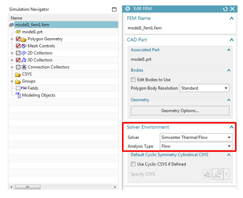
Figure 2: Creating the Thermal/Flow fem

Then create a 3D mesh for the air volume, as shown in Figure 3.

Figure 3: Mesh the air volume only. The structure is not meshed.

3.     Create the Flow Solution

We now create the “Simulation” file, and define a “Flow” analysis. As shown in Figure 4, define a non-turbulent transient analysis. Furthermore, in the “Result Options”, see Figure 5, check the “Pressure and Shear Resultants” box – these will be used for the mapping step.

Figure 4: Flow Solution setup

Then, edit the “Transient Setup” tab as illustrated in Figure 5. 

Figure 5: Results Options for flow forces

Figure 6: Transient setup options

4.     Apply the boundary conditions.

Three boundary conditions are applied:

An inlet of 30 mm/sec at ambient conditions on the –Y faces.

An opening at ambient conditions on the +Y faces.

Slip walls to represent an extended fluid domain on the +X, -X and +Z faces.

As nothing is prescribed on the bottom surface, the solver automatically assumes no-slip, which represents a solid surface. Boundary conditions are shown in Figure 7.

Figure 7: Boundary conditions

We now solve this Flow solution. An example of the flow velocity profiles is shown in Figure 8.

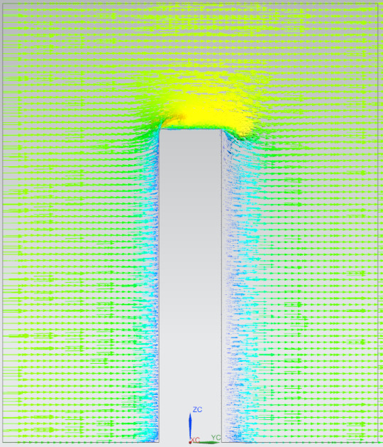
Figure 8: Flow velocity profile.

Mapping the flow forces

1.     Create the structural mesh

Starting with the same part created in step 1, create a new fem file. In the “Edit FEM” window, make sure to choose the NX Nastran (Structural) “Solver Environment”, as shown in Figure 9.

Figure 9: Creating the Structure fem

This time, we will only mesh the structure component and ignore the air volume. See Figure 10. An aluminum material is assigned to the tube.

Figure 10: Structure mesh only. The air volume is not meshed.

2.     Create the Mapping Solution

To map the flow forces to the structural analysis, create a new “Simulation” file and choose a “Thermal-Flow” Solution with a “Mapping” type, as shown in Figure 11. If you leave the “Transient Times” table empty, the solver automatically selects all transient time steps from the flow solution.

Figure 11: Create a Mapping Solution

Next, in the “Optional Output” tab, check the boxes shown in Figure 12 to create the mapping and target Nastran structural solution. A static solution is created. This type of analysis is valid when inertial effects are negligible and where the dynamic content of the flow pressures is well separated from the structures principal modes.

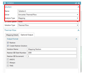
Figure 12: Creating the Mapping and Nastran Solution

3.     Solve the Mapping Solution

Before solving the Mapping Solution, we define a “Mapping Target Set”. This defines the surfaces on which the flow forces will be mapped. Select the cylindrical face of the tube and its free face, as shown in Figure 13 and Figure 14. We can now solve the Mapping Solution. An example of the mapped forces at a given time step is shown in Figure 15.

Figure 13: Mapping Target Set

Figure 14: Select the mapped surfaces

Figure 15: Example of mapped forces

4.     Solve the structural solution

The “Simulation Navigator” now shows one subcase corresponding to each transient time step of the flow solution. See Figure 16.

Figure 16: Subcase created for each transient time step of the flow solution

Before solving, we fix the translational degrees of freedom on the –X face of the tube. Solve the solution.

5.     View displacement results

Next, select a subcase and display the displacement results, as shown in Figure 17. The deformed structure is shown together with the undeformed mesh in Figure 18.

Figure 17: Nodal displacement results

Figure 18: Deformed and undeformed structure

[mechanicalengineeringblog]

How to simulate delamination using cohesive elements in Simcenter Multiphysics

Quick Overview

Cohesive elements are special-purpose 3D elements used to model adhesive joint failure as well as delamination of composite plies. You can create cohesive elements between pairs of geometric surfaces and between specific plies, in both the Simcenter Multiphysics and Samcef environments of Simcenter 11 Pre/Post.

In what follows, we focus on the Simcenter Multiphysics environment and describe how to create cohesive elements between plies in a global layup, in order to simulate delamination using a 3D laminate composite model.

Introduction to cohesive elements in Simcenter Multiphysics

In this environment, cohesive elements can be used to:

Model delamination between plies in a laminate composite.

Simulate the presence of an adhesive between bonded surfaces. Cohesive elements offer several advantages over traditional glue-type connections, especially in situations where the integrity and strength of the connection are of interest.

Several options exist to include cohesive elements in an analysis:

You can use the “3D Swept Mesh” command with type set to “Manual Between”, in order to create a layer of cohesive elements between specified source and target faces. If the source and target faces are coincident, the software generates zero thickness cohesive elements.

You can use the “Element Extrude” command with the type set to “Element Faces”, in order to manually generate cohesive elements.

You can use the Simcenter Laminate Composites’ “Layup Modeler” dialog to create cohesive layers between specific plies.

The cohesive element’s material type can be “Isotropic”, “Orthotropic” or ”Damage Interface”. The “Damage Interface” material type evaluates the cohesive layer integrity during the nonlinear solution. You can use options in the “Damage Interface” material dialog box to specify, amongst others, the damage estimation model.

For more information, see Simcenter Multiphysics “Damage Interface” material and Samcef “Damage Interface” material.

Create a cohesive element layer

We begin with an inflated 3D laminate, as shown in Figure 1.

Figure 1: Example of an inflated 3D laminate

1.     Create a “Damage Interface” material

Using “Manage Material”, create a “Damage Interface”-type material, as shown in Figure 2.

Figure 2: Defining a "Damage Interface"-type material

Enter the fracture toughness and stiffness for each of the 3 failure modes: these properties are derived from tests. In this case, we use an exponential-type damage law. See Figure 3:

Figure 3: Interface constitutive behavior and properties

2.     Create cohesive elements between plies

In the “Layup Modeler”, shift-select two ply groups and click the “Create New Cohesive Layer” button.

Figure 4: Create a cohesive layer

Then, assign the previously created “Damage Interface”-type material to the cohesive layer. This is illustrated in Figure 5.

Figure 5: Assign the created material to the cohesive layer

Setting up the simulation

1.     Create the simulation and solution

Create a new Simcenter Multiphysics simulation and solution, keeping “Automatically Create Step or Subcase” checked:

Figure 6: Create a Simcenter Multiphysics solution

In the “Solution Control” tab, check the “Material Nonlinearity” box (See Figure 7).

Figure 7: "Solution Control" tab

From the “Result Options” tab, edit the “Structural Output Request” (see Figure 8):

Set the “Damage” of the Cohesive Element Results to “DAMAGE”.

Set the “Output Medium” of the Cohesive Element Results to “PLOT”.

Figure 8: "Output Request" menu

2.     Define the boundary conditions

The -X face of the coupon is completely fixed, while Mode 1 delamination is solicited by defining equal and opposite 1 mm displacements to the top and bottom nodes of the +X face. This is shown in Figure 9 and Figure 10.

Figure 9: Fixed Constraints and Enforced displacements

Figure 10: Constraints in Sim Navigator

3.     Define the time step

To define the time integration parameters, select the “Step – Nonlinear Static” node in the sim navigator, then right-click “Edit”, and in the “Time Step Definition” tab, set the “End Time” to 1 sec and the “Number of Increments” to 20. See Figure 11 and Figure 12.

Figure 11: Edit the time integration controls

Figure 12: Specify solution time and time step

4.     Run the simulation and animate the damage results

Next, launch the solution and subsequently load the “Cohesive Damage [EXPO] – Element Nodal V1” results. In the “Post Processing Navigator – Fringe Plot”, display only the cohesive elements, as shown in Figure 13:

Figure 13: Display the cohesive elements

To animate the results across all the iterations of the nonlinear solution, use the “Animate” button in the ribbon bar. A damage value of 1 indicates a complete delamination of the plies. Use the animation options shown in Figure 14:

Figure 14: Animate the results

Figure 15: Animation of the delamination results.

[mechanicalengineeringblog]

How to create 3D solid mesh for a sandwich composite laminated car hood using Simcenter Laminate Composites

Quick Overview

Sandwich panels are prevalent in many structural applications. The panel facesheets react the membrane and bending loads, whereas the core reacts the bulk of the transverse shear loads. Therefore, you may use the solid mesh to get better results in the ply out-of-plane direction to evaluate delamination and also investigate the local sandwich behavior near the tapered core.

This tips and tricks shows how to use Simcenter Laminate Composites to create a 3D mesh of a tapered laminated composite sandwich car hood.

Figure 1: Car hood CAD model. Top face (left). Bottoms face (Right).

Steps

1-    Create a 2D mesh

First, we create the parent 2D mesh on the car hood top face and that will be extruded to a 3D mesh. To create the 2D mesh, go to Home tab, under Mesh group, select 2D Mesh command to create a 2D mesh on the top face of the car hood.

Figure 2: Create 2D mesh on the car hood top face.

We use a ply-based approach to define layups’ global plies and how they drape on the model. In the Laminate tab, select Laminate Physical Property. In the Laminate Modeler dialog, set the stacking recipe to Inherited from layup and click OK.

Figure 3: Create a Laminate Physical Property.

Let’s assume a simple quasi-isotropic [0/45/-45/90]s layup with a 12.7 mm thick foam core, which is tapered around the perimeter of the hood.

In the Laminate tab, select Global Layup and then in the Layup Modeler dialog, select the Import Layup Using Shorthand Format.

Figure 4: Create a Global Layup.

In the shorthand Format dialog enter the layup as [0/45/-45/90/0’]_s, set the Thickness to 0.125mm and the Material to CFRP.

Figure 5: Input the layup using shorthand format.

In the Layup Modeler dialog, verify the Stacking Recipe is Symmetric with core, change the material for Ply 5, which is the core, to foam and change its thickness to 12.7mm.

Figure 6: Layup definition in the Layup Modeler dialog.

To drape the plies, shift-select plies 1 to 4 and click on the Define Draping Input command. In the Draping Data: Layup Files dialog, select the entire top face of the car hood, and click OK.

Figure 7: Drape the plies on the car hood.

In the Layup Modeler dialog, select the core ply and then click on Define Draping Input command. This time select the face(s) on which the core ply is going to be laid up.

Figure 8: Drape the core ply.

The 2D layup is now defined and properly draped. To automatically inflate this layup to a 3D mesh, go to the Laminate tab, select Extrude Laminate command.

Figure 9: Extrude laminate command.

In the Laminate 2D-to-3D Extrusion dialog, under the Settings group, select all the faces of the car hood on which the 2D laminate is draped.

Figure 10: Laminate Extrusion settings.

Under the Sandwich Inflation group, Set the Top Skin Mesh and Bottom skin Mesh to 3D and select the core ply from the list. Here you can also optionally set the Number of Core Element Layers. Click Ok.

As shown in Figure 11, the 3D solid mesh for the car hood is created. Drop-off resin elements are automatically created where the core tapers. The drop-off resin elements are created as a separate mesh entity. You can drag the resin meshes to be under the same collector as the core meshes.

Figure 11: 3D mesh created for the laminated composite car hood.

[mechanicalengineeringblog]

How to perform random analysis of mixed laminated composite – metallic structures

Quick Overview

The laminate dynamic simulation random event reads the results from an NX Nastran SOL 103 real eigenvalues solution and uses an efficient modal approach and advanced integration algorithms to efficiently produce accurate peak responses that correspond to the specified confidence level.

This tips and tricks shows how to use Simcenter Laminate Dynamics to quickly evaluate the behavior of a satellite antenna assembly subjected to the base-driven random excitation function shown in Figure 1. The input power spectral density has an irregular shape because it has been notched using a force-limited vibration approach, in order to avoid overtesting at the fundamental X-axis mode of the antenna.

Figure 1: Excitation PSD curve.

Steps

1.     Create the parent structural solution

First, define the FEM of the satellite antenna in Simcenter. The reflectors, intercostal structure and sub reflectors are made of composite laminates, the waveguide is made from aluminum, and the brackets are made of titanium.  Failure of the metallic components will be established using Von Mises stresses; failure of the composite plies will be established using the classical Tsai-Wu failure criterion.

Figure 2: Satellite antenna model.

Then, create a Nastran SOL 103 Real Eigenvalues solution. You must set Solution Process to Laminate Dynamics on the General tab in the Solution dialog.

Figure 3: Set the Solution Process to Laminate Dynamics.

2.     Constrain the structural solution

The laminate dynamics solution process simulates a base excitation; therefore, there should be a single excitation point in the model. In a case where there are multiple constraints in a model, you can connect all of those interface degrees of freedom to a single node using a rigid element and then fix the single node.

In the satellite antenna example, Figure 4 shows that the three inner intercostal supports are all connected to a single, constrained node using an RBE2 element.

Figure 4: Create a single excitation point.

3.     Specify structural output request

Laminate Dynamics Simulation computes results starting from those Nastran results that are stored in the parent OP2 file. To request results output in the OP2 file when you solve the Nastran solution, you need to create a Structural Output Request modeling object.

All ply and interlaminar failure theories require the stress output request except the maximum strain ply failure theory, which requires the strain output request. In order to process displacements, accelerations, and velocities only the displacement request is required.

To create/modify a Structural Output Request, in the Solution dialog select Case Control and then select Structural Output Request.

Figure 5: Create/modify structural output request.

As a general rule you should retain, at a minimum, all the modes with resonant frequencies that lie within your random input lower and upper frequency bounds. For better accuracy, you should retain all modes up to a frequency that is at least twice your upper bound.

In the Solution dialog select Case Control and then select Lanczos Data. In the Real Eigenvalue dialog enter the required frequency range.

Figure 6: Define the frequency range for SOL103 eigenvalue solution.

In this example, the PSD excitation in Figure 1 is between 20 Hz and 2000 Hz, so as a minimum all the modes with frequencies in this range should be retained. We run the solution between 0 and 2000 Hz. We then perform a quick modal summary analysis using Structural Analysis Toolkit for Nastran (SATK) to evaluate the modes’ effective mass, an indication of the amount of mass that coherently participates in each mode that also is a conservative criterion to define the cut-off frequency. The modal summary result, Figure 7, shows that the cumulative effective mass in each axis is above 98% of the antenna’s rigid body mass: It is therefore not necessary , to calculate modes up to 4000 Hz (twice of the upper limit of the PSD excitation frequency), saving time and resource in the running Nastran Solution 103.

Figure 7: Modal summary analysis by SATK.

It is worth mentioning that if you do not retain enough computed modes for your frequency response range, you can account for modal truncation effects by invoking either a residual vector or a residual flexibility approach.

4.     Set up a Laminate Dynamics solution process

When the Nastran Solution 103 is completed, in the Laminates tab click on Laminate Dynamics. In the Laminate Dynamics dialog, define a name for the solution, select the parent structural solution from the list, and click OK.

Figure 8: Create a Laminate dynamic solution.

In the Simulation Navigator, expand the Dynamic simulation node and click on the Normal Modes node, which shows the number of modes used in the dynamic solution. Expand the Laminate Dynamics Detail View, you can optionally select a subset of the modes that Nastran computed.

Figure 9: Modes used in dynamic simulation and their assigned damping value.

You can edit the damping value for each mode individually by editing the value in the Laminate Dynamics Detail View. To edit the damping value for all the modes, in the Sim Navigator right-click on the Normal Modes node and select Edit All Damping Factors. In the Edit Damping Factor dialog enter the viscous damping value.

Figure 10: Assign/edit damping factor.

5.     Create a random or sine event

To create a random event, in the Laminates tab, click on the Random Event.

Figure 11: Create a random event.

In the Random Event dialog, under the Excitation PSD tab, click on the use a function icon, where you can browse for the already defined function.

Under the Analysis Parameter tab, set the lower and upper bound of the frequency solution, which can be a subset of the frequency range of the input function. You also need to define the desired confidence level. We used 99.73% confidence, which corresponds to the 3 times the standard deviation which is an industry default.

Figure 12: Random event base input and settings

From the Random Event dialog, you also define the Laminate Random Output Requests modeling object in which you specify the desired output requests. A wide range of outputs can be simultaneously requested. In this case, we request failure metrics only.

Enable Homogenous will compute failure metrics for elements that reference homogeneous materials. The Laminate Dynamics solution uses the peak Von Mises stress to compute the failure index and the margin of safety. The peak Von Mises stress correctly accounts for the phases of the constituent stress tensor components, and corresponds to the confidence level specified previously: there is no need to manually multiply by the number of standard deviations.

Enable Layered computes failure metric results for elements that reference a laminate physical property or a solid laminate physical property. The equations for failure index, strength ratio, and margin of safety depend on the failure theory that you selected in the Laminate Modeler when you defined the layup in the FEM. In this case we have specified the Tsai-Wu failure criterion, which uses a second order equation composed of the stress tensor components. Simcenter Laminates accounts for the phases between the components when accurately computing failure indices, strength ratios as well as margins of safety on a ply-by-ply basis. The failure metrics also correspond to the desired confidence level.

Figure 13: Output request for random dynamic analysis.

To solve the Laminate Dynamics event, in the simulation navigator, right-click on the Random event and select Solve. When the solution complete, the results can be viewed in Post Processing Navigator.

Figure 14: Plot of Ply 1 strength ratio.

Figure 15: Plot of Von-Mises stress in metallic parts.

[mechanicalengineeringblog]

Approaches to Laminate Buckling with Simcenter

Quick Overview

Although it is well known that Simcenter supports linear buckling solutions (SOL 105), some engineers are reluctant to use this method for composite laminate, based on the perception that the linear buckling analysis does not adequately account for the low transverse shear stiffness of the laminate and is thus not-conservative. This paper demonstrates that Simcenter linear buckling analyses are, in fact, adequate for composite laminates, even for sandwich structures.

Background

Buckling of plates inherently involves large transverse deflections and out-of-plane bending, for which transverse shear becomes significant. Since composite materials have relatively low transverse shear stiffness compared to their in-plane properties, standard plate buckling equations will overestimate the buckling strength of composite laminates.  This error will be larger for thicker laminates.  This behavior is well known to composite structural analysts and nothing new has been presented thus far.

There is this persistent belief among some engineers that the linear buckling solution implemented in engineering simulation software suffers from the same deficiency.  They will instead prefer to use a non-linear finite-element solution to determine the buckling strength of a laminate.  The idea is that the gradually applied load during the non-linear solution will cause it to stop converging when the buckling strength has been exceeded.

This non-linear approach is sound, but does have some caveats:

The onset of instability must be artificially introduced for flat surfaces;

The model could stop converging for reasons other than buckling of the structure, requiring additional interpretation;

The non-linear solution takes more time to solve (Many load steps are needed for an accurate prediction);

The question is therefore whether or not the non-linear approach is worth this extra effort (i.e. Are the results from the linear buckling approach actually not conservative?).

Problem Definition

We will now investigate a buckling problem with the two approaches previously discussed using Simcenter.  Let us begin with a simple 18in by 10in flat plate simply supported on three edges as shown below:

In this first example, we will define an 8-ply laminate [45/0/-45/90]S of T300/5208 (Properties used shown below).

We set-up the boundary conditions as:

At this point, we can readily perform a linear buckling analysis (SOL 105), where we predict a first buckling mode at 181.3lbf (200lbf applied * 0.906538).

We will now verify whether or not we get similar results with a non-linear analysis.  First, because we have a perfectly flat plate, we must artificially introduce the onset of instability by slightly moving a node out of the plane of the plate.  We thus translate a node near the center of the plate as shown below:

If this step was not done, the plate would most likely simply compress but would not bend out of its initial plane.

We now set-up the non-linear solution (SOL 106), selecting the global iterative solver.

Then we set a large number of increments (100 here) and change the convergence criteria as Displacement and Work.

Finally, we change the parameters to account for large displacements:

In order to achieve buckling, the applied load must exceed the critical load. If the applied load is insufficient, we will not know how close to buckling we are.  We set the applied load to 250lbf, well above the critical load predicted by the linear buckling solution.

The last increment of the solution to converge is the 72nd. As a result, we calculate the critical load as 250lbf*72/100=180lbf.  The next increment would have corresponded to a load of 182.5lbf.  We can see that the critical load predicted by the linear buckling analysis fits right between these two values.  At first glance, it seems that linear buckling solution is no less conservative than the non-linear solution.

Let us change the lay-up to [(-45/90/45/0)S_2]S, increasing its thickness to 32 plies as to generate a fair amount of transverse shear stresses.  The linear buckling solution now predicts a critical load of 10,746.6lbf.  Applying 11,000lbf to the non-linear model, we obtain convergence up to increment 97, corresponding to a load of 10,670lbf. This is again just below the SOL 105 prediction.

If we further add a honeycomb core (5056, 3/16” cells, 3.1PCF, 1/8” thick) to the center of this laminate, we increase the buckling critical load to 30,202.8 (according to the SOL 105).  Applying 31,000lbf to the non-linear model, we obtain convergence up to increment 97, corresponding to a load of 30,070lbf.

Conclusion

With these 3 tests, we have shown that the only conservatism coming from using a non-linear solution is due to the incremental nature of the load application.  Indeed the last load for which convergence is observed was found to be below the critical buckling load.  Note that this may not always be the case, depending on the load applied and the number of increments selected to run the non-linear model. Nevertheless, this exercise has shown a clear relation between the results of a linear buckling analysis (SOL 105) and a non-linear analysis (SOL 106), both performed with Simcenter.

The results of a Simcenter linear buckling analysis (SOL 105) can therefore be considered as sound for composite laminates and sandwich panels.  One should however be mindful that this may not be the case for other simulation suites.  Also, analysts should also consider that other failure modes may, in fact, be the critical ones in certain situations (e.g. delamination, core failure…). These failure modes would not necessarily be exposed in either a SOL 105 or a SOL 106.

[mechanicalengineeringblog]

How to preview NX NASTRAN contact and glue regions

Quick Overview

When you define a contact or glue condition in your model, NX Nastran internally creates contact or glue elements using the contact or glue regions you select as well as the search distance that you define. Although these contact or glue elements may become inactive as NX Nastran iterates, it can be helpful to verify where those elements are actually created.      

NX Nastran optionally generates a bulk data file containing dummy meshes representing the source and target elements used by a given contact or glue set: there are as many preview bulk data files as there are contact and glue sets in the solution. The bulk data file(s) can be imported into NX for display.

Note that for both contact and glue conditions, NX Nastran writes the preview output when it evaluates the initial contact or glue condition. This occurs before any loading is applied to the model.

Steps

1.     Define contact and glue in the model

First, define all the contact and glue conditions in your model, and add them to your active solution. Then, in the Sim Navigator, right click on the solution and select Edit. In the Solution dialog, select Case Control. To request export of the contact preview, follow step 2.1; to request export of the glue preview, follow step 2.2.

Figure 1: Solution dialog.

2.1. Request a contact preview output

To request creation of the contact preview, in the solution dialog, click on Create Modeling Object for Global Contact Parameters.

Figure 2: Create global contact parameter object.

In the Contact Parameter dialog, under the Secondary Parameters group, set the Export a Preview Bulk Data File (PREVIEW) to Yes, and click OK.

Figure 3: Contact parameters dialog.

2.2. Request a glue preview output

Similarly to the previous step, to request export of the glue preview, in the solution dialog, click on Create Modeling Object for Global Glue Parameters.

Figure 4: Create global glue parameter object.

In the Glue Parameter dialog, set the Export a Preview Bulk Data File (PREVIEW) to Yes, and click OK.

Figure 5: Glue parameters dialog.

3. Solve the model

At this step, simply solve the model: The preview file is created in the solution directory with the following naming convention:

For Contacts:

<input_file_name>_cnt_preview_<subcaseid>_<contactsetid>.dat

For Glues:

<input_file_name>_glue_preview_<subcaseid>_<gluesetid>.dat

For example, if the solution name is test, the subcase id is 101, the contact set id is 201, and the glue set id is 301, then the preview file names will be

test_cnt_preview_101_201.dat

test_glue_preview_101_301.dat

4. Import the preview file into NX

The procedure of importing the preview file into NX is similar to importing an NX Nastran bulk data file and is the same for both contact and glue preview files.

To import the preview file, from the File menu, select Import and then choose Simulation.

Figure 6: Import the preview bulk data file.

In the Import dialog, select NX Nastran and click OK.

Figure 7: Import dialog.

In the Import Simulation dialog, browse for the preview file and click OK.

Figure 8: Import simulation dialog.

When the simulation is imported, in the Sim Navigator, you will see the dummy meshes representing the source and target regions used for contact or glue definition.

For example, in the model of Figure 9, the complete bottom face is selected by the user as the contact source region. However, due to the Max Search Distance of 2mm in the contact definition, only a subset of those elements is considered by the NX Nastran solver (Figure 10).

Note that at the end of a solution, some contact elements may become inactive because they did not participate in the converged condition. To view the locations of the final active contact elements, you can request contact tractions with the BCRESULTS case control command, and then view them in a post processor.

Figure 9: Contact definition in a sample model.

Figure 10: Contact preview imported into NX.

[mechanicalengineeringblog]

How to create a 4D field in Simcenter

Quick Overview

You may have to define a load or a boundary condition that not only varies as a function of spatial coordinates, but also with time, temperature, or frequency. This Tips & Trick shows how to use Simcenter to create a 4D field, which allows you to model a functional expression of the form:

f = f(x1,x2,x3,α)

where x1, x2, and x3 represent a set of cartesian, cylindrical, spherical, or parametric spatial coordinates, and α represents a non-spatial variable like time, temperature, or frequency.

If the 4D functional relationship can be expressed as a closed-form mathematical expression, you can create the 4D field as a formula field. When Simcenter evaluates the formula field for a given set of spatial and non-spatial values, it simply evaluates the expression that relates the independent and dependent domains at the given values.

If the 4D functional relationship can be approximated by a set of tabular data that relates the independent and dependent domains, you can create the 4D field as a table field. When Simcenter evaluates the table field for a given set of spatial and non-spatial values at which a tabular data point does not exist, it interpolates the tabular data to obtain the corresponding dependent domain value. You can select the interpolation method that the software uses to look up values.

In this example we will show how to use a 4D formula field in Simcenter to model the footprint pressure of a roller traveling on a track.

Figure 1: Model the foot print pressure of a roller travelling on a track.

Figure 2: Varying pressure with spatial coordinates and time.

Steps

Let’s assume that the roller travels at a speed of 3 mm/sec and has a foot print pressure of 9 mm length (in the X axis) with a maximum pressure of 45 MPa.

1. Create a field of varying spatial coordinates with time  

Since the roller is moving at a constant speed of 3 mm/sec, the roller’s central location can be simply calculated using the following function:

X = 3*t

To create this field, in the Simulation Navigator right click on the Fields node and select New Field, Formula.

Figure 3: Create a formula field.

In the Formula Field dialog, under the Name group, enter a meaningful name, for example, X_Center. Then under the Domain group, set the Independent to time and Dependent to Cartesian.

Since in our model the position of the roller changes only along the X axis,  under the Expression group, select x and in the Rule Formula box type:

3[mm/sec]*time

Figure 4: Create a formula field for position of the roller with respect to time.

By end of this step, we defined the varying position of the roller with respect to time. So, we can now proceed to define the pressure field.

2. Create a field for the pressure

We assume that the roller footprint pressure is maximum at its center and linearly decreases toward the fore and aft edges of the foot print, in the X direction. The pressure is constant in the other direction on the surface.

Figure 5: Roller footprint pressure distribution.

To define a field for the pressure, in the Simulation Navigator right click on the Fields node and select New Field, Formula.

In the Formula Field dialog, under the Domain group, set the Independent to time,Cartesian and Dependent to Pressure. You will notice that the independent variables and the field created in the step1 are listed under the Expression group.

We assumed the roller foot print pressure has a length of 9 mm. So, the the pressure formula can be defined as  

if ( abs(x-fd("X_center","x"))<=4.5) Then (10*(4.5-abs(x-fd("X_center","x")))) Else (0)

where x is the independent variable, and X_center is the position of the roller, which is varying with time according to the field defined in step 1. Note that to use a value from another field, you need to use the fd(“Fieldname”,”value”) command.

Figure 6: Define a formula field for the roller foot print pressure.

3. Define the pressure load

To define the pressure load, in the Simulation Navigator, right click on Loads, and select Pressure.

Figure 7: Define the pressure load.

Figure 8: Pressure dialog.

In the Pressure dialog, under the Model Objects group, select the track bed face as the location where the pressure should be applied. Under the Magnitude group, click on the equal sign, and then choose Select Existing Field.

Figure 9: Fields dialog.

In the Fields dialog, select the Formula Field, which was defined in Step 2. Click OK on all dialogs.

4. Verify the defined pressure (Optional)

By the end of step 3, the varying pressure with respect to spatial coordinates and time is already defined and can be used in a solution. Simcenter allows you to plot and animate the applied load to verify whether it is correctly defined and applied to the model.

To plot the varying pressure load, in the Simulation Navigator, right click on the pressure load and select Plot Contours.

Figure 10: Plot load contours of the applied pressure.

Figure 11: Boundary Condition Contour Plot dialog.

In the Boundary Condition Contour Plot dialog, under the Selected Boundary Conditions group select the pressure load. Then under the Plot Options group set the Plot Type to Animation, and Independent Variable to Time. Set the Start, Stop, and Number of Frames to 0, 100, and 33, respectively. Click on the Plot icon.

Figure 12: Contour plot of the applied pressure.

[mechanicalengineeringblog]

How to optimize a laminate in Simcenter

Quick Overview

Simcenter Laminate Composites (LC) allows you to optimize the fundamental properties of a laminate coupon- for example, increasing its modulus in the X direction, minimizing its mass or its thermal expansion- by modifying ply angles, ply thickness, ply materials or by removing plies.

Core content

The optimization works on a single laminate physical property and involves three components: design variables, design constraints, and design objectives. The property does not have to be assigned to a collector.

Design variables

LC supports the following types of design variables for the plies of a laminate property:

Ply thickness

Ply angle

Material assigned to the ply

Ply existence, ie whether or not a ply can be removed from the laminate

Ply thickness and ply angle design variables can be either discrete or continuous. Ply materials and ply existence are inherently discrete design variables.

Design Constraints

LC supports the following types of design constraints on a laminate:

The total mass of the laminate

The buckling factor for a plate of a given coupon size

The ply failure index

The natural frequency for a plate of a given coupon size

The ply contiguity

The equivalent laminate X and Y Young's modulus

The equivalent laminate shear modulus

The equivalent laminate Poisson's ratio

The equivalent laminate X, Y, and XY thermal expansion coefficients

Design objective

LC supports the following design objectives:

The total mass of the laminate

The buckling factor

The equivalent laminate X and Y Young's modulus

The equivalent laminate shear modulus

The equivalent laminate Poisson's ratio

The equivalent laminate X, Y, and XY thermal expansion coefficients

Steps

In this example, we are going to use LC to minimize the mass of a deployed solar array with constraints on the minimum natural frequency and equivalent longitudinal stiffness of each individual solar array panel. The design variables are the ply thickness, ply angles, and ply existence. LC optimization is well suited for the flat, rectangular geometry of the array panels, even if the assumed boundary conditions are not fully representative of the actual design.

Figure 1 Spacecraft with deployed solar panels

Each solar array panel is initially designed with a 12 mm thick aluminum honeycomb core, and symmetric 4-ply CFRP face sheets [0/45/90/-45]s, in which each ply is 0.127 mm thick. The initial design has a mass of 0.77 kg, an equivalent longitudinal stiffness of 8.79 GPa, and a natural frequency of 76 Hz. The optimum design should have an equivalent longitudinal stiffness similar to or greater than the initial design and with a natural frequency of at least 20 Hz.

Define the laminate

To define the laminate properties, In the Laminate tab click Laminate Physical Property to define the laminate layup.

Figure 2: Define laminate layup

Figure 3: The initial design of solar array laminate.

First, we need to define design variables. In the Laminate Modeler dialog under the Optimization group check Enable Optimization. As a result, a new group is displayed under the ply layup definition table.

Figure 4: Enable laminate optimization

Define design variables

The design variables for this example are ply angles, ply thickness, and ply existence. To define a design variable for a ply angle, under the Design Variable Manager group, set the Type to Ply Angle and click

In the design variable specification dialog, specify a name for this design variable, set the Domain Type to Continuous, and set the Min and Max to -90 and +90, respectively. Click OK.

Figure 5: Define design variable for the angle of ply 1

Since the angle of each ply can vary independently from the other plies, we need to repeat this process 4 times to define ply angle design variables for each ply. Note that we do not need a ply angle design variable for the core.

To define design variables for ply thickness, under the Design Variable Manager group, set the Type to Ply Thickness and click

In the design variable specification dialog, specify a name for this design variable, set the Domain Type to Continuous, and set the Min and Max to 0.0508 mm and 0.254 mm, respectively. Click OK.

Figure 6: Define design variable for the thickness of ply 1

Similarly to the ply angle design variables, we need to repeat this process 4 times to define ply thickness design variables for each ply. For the core ply, create an additional ply thickness design variable, where the limits of Min and Max are 8 mm and 25 mm, respectively.

To assign design variables to a ply, in the Laminate Modeler dialog, select the ply and under the Assign Design Variable group, select the relevant ply angle design variable from the Angle DV drop down menu, which lists all the defined ply angle design variables. Similarly, to assign a ply thickness design variable use the Thickness DV drop down menu, which lists all the defined ply thickness design variables. Repeat the above process and assign the relevant design variables to all the plies, including the core ply.

We want to keep the outer ply for the final design, but the rest of the plies can be removed by the optimization algorithm. To identify plies 2, 3, and 4 as removable, select them and check Removable Ply.

Figure 7: Assign design variables to a ply

Note that when a design variable is assigned to a ply, an asterisk appears in the relevant column of that ply. For example, in Figure 7, it can be seen that an asterisk is added beside the thickness and ply angles for ply 1. Also for plies 2 to 4, there is an asterisk beside the ply id, indicating these plies are removable.

Define objectives and constraints

Under the Optimization group, click

to open the Laminate Optimizer dialog.

Figure 8: Laminate Optimizer Configuration dialog

In the Laminate Optimizer Configuration dialog, under the Opt Design Space tab, and under the Objectives group, click

to define the objectives. In the Objective Specification dialog, set the Type to Total Mass and set the Rule to Minimization, and click OK.

Figure 9: define design objective

To define the constraint, in the Laminate Optimizer Configuration dialog, under the Opt Design Space tab, and under the Constraints group, click

In the Constraint Specification dialog, set the Type to Natural Frequency, and set the Rule to Greater or Equal to Limit. In the Limit box enter 20 Hz and click OK.

Figure 10: Define design constraint on minimum natural frequency

Repeat the process above and create a new constraint that the minimum Young’s Modulus along X direction should be greater than 6.67 GPa as shown in Figure 11.

Figure 11: Define design constraint on minimum Young's Modulus

Then, under the Plate Properties group, enter the plate size as 1050 mm for Side A and 325 mm for Side B. Click Ok.

Figure 12: Plate properties

Note: The optimization in LC has two optimization algorithms: Standard and Hybrid genetic algorithm. The parameters for the optimization algorithms can be tuned under the Operators, Basic Params, and Advanced Params Tabs. In this Tips and Tricks, we will use the default settings.

Launch the optimization process

In the Laminate modeler dialog, under the Optimization group, click

to launch the optimization process. To see the best five optimum candidates and a summary of the optimization results click

which exports the optimization results to a spreadsheet. You can also check the detail box, to have the layup and laminate properties for each of those five optimum candidates.

A summary of the optimization results is shown in Figure 13. It can be seen that optimization algorithm removed 2 plies, reduced the mass by about 58% while satisfying both constraints.

Figure 13: Summary of the optimization results

Finally, using the Results drop-down menu, you can choose one of the candidate optimum designs and the laminate definition is automatically updated to the layup of the selected optimum design (Figure 14).

Figure 14: Select one of the five optimum candidates

[mechanicalengineeringblog]

Quickly Determine Laminate Coupon Test Loads using NX Laminate Composites

Demo Video:

Quick Overview

NX Laminate Composites (NXLC) allows you to easily define laminates, assign them to 2D or 3D meshes of complex geometries, and post-process composite failure metrics. For simple parts like test coupons, creating a FEM is not required, as NXLC allows you to verify the ability of your laminate to withstand the following loading conditions:

Membrane forces

Bending moments

Transverse shear forces

Temperature loads

In this example we will determine the loads required to produce first-ply failure in a 4 point bending test coupon as per ASTM D7264. We will compare the NXLC results with those of a shell element FEM with appropriate boundary conditions.  

Laminated strip under four-point bending

Figure 1: Laminate strip under three-point bending

A cross-ply laminate with [0/90/0/90/0/90/0] layup is specified with the center ply being four times as thick as the others. With such a lay-up, the bending moment is reacted more uniformly across the section. A model, with appropriate boundary conditions, is used and predictions are obtained using laminated shell elements.

Figure 2: A laminate test specimen under four point bending

The initial guess at the failure bending moment is 1250 Nmm. The applied moment per unit length is 1250 N.mm/10mm = 125 N

The applied load P = -4M/L = -(4*1250Nmm)/50mm= -100 N.

1.       Determine failure load Using NXLC

Create a new empty FEM, by clicking NEW command.

Figure 3: Create a new FEM

First, we define the material properties to be used in the laminate definition.

Go to Home tab and under the Properties group click on Manage Materials.

Figure 4: Manage Materials

In the Manage Materials dialog, set the type to Orthotropic and click on Create.

Figure 5: Define a new orthotropic material

Then define mechanical and strength properties as shown in Figure 6 and Figure 7.

Figure 6: Define material mechanical peroperties

Figure 7: Define material strength properties

To define the laminate, go to NX’s Laminates tab and click the Laminate Physical Property button.

Figure 8: Create a laminate physical property

In the laminate modeler, select Import Layup Using Shorthand Format button to quickly define the layup.

Figure 9: Import Layup Using Shorthand Format button

Figure 10: Shorthand format to define a layup

In the Laminate Modeler dialog, set the output format to PCOMP, and the Ply Failure Theory to Tsai-Wu. Click OK to close the dialog.

Figure 11: A symmetric quasi-isotropic laminate [0/90/0/90/0/90/0]

In the Laminate Modeler, under the Validation group, click the Analyze Laminate Strength button.

In the Laminate Strength Analysis dialog, enter the vaue of 125 N for X Bending Moment per unit length and click on Export Spreadsheet to generate the analysis results.

Figure 12: Define applied load in Laminate strength Analysis dialog

In Laminate 1 spreadsheet, navigate to Strength Analysis worksheet to see the analysis results.

Figure 13: A preview of a portion of the results generated by NX Laminate Composites.

Figure 14: A preview of a portion of the result summary generated by NX Laminate Composites.

The minimum strength ratio for all plies is 1.185, which means the coupon will fail at a load of 1.185*1250Nmm=1481.25 Nmm, which is equal to a stress resultant of 1481.25Nmm/10mm=148.125N (shown in the spreadsheet results under the Allowable Loads on Laminate. Note that the slight difference is due to round off in spreadsheet).

Keep your FEM open in NX.

2.       Determine failure load using FEM

2.1.          Create the Coupon Geometry

In the simulation navigator, make your part file the work part, and create a rectangular face with dimensions 60 mm x 5 mm, representing a half of the test specimen.

Figure 15: Create geometry in NX

To create a FEM and Sim, go to Application tab and click the Advanced button.

Figure 16: Create a FEM and Sim

In the sim navigator, right-click on the model and select New FEM and Simulation. Select the sheet body you just created and click OK.

Figure 17: Create a new FEM and Sim

Then, make the FEM work Part and create a 2d mapped mesh with 1 mm CQUAD4 element size.

Figure 18: Meshing the geometry with 2D shell elements

2.2.          Assign the Laminate Property to the Mesh

Import the physical property and the material you created in your first FEM: From the Menu, Insert, Append FEM:

Figure 19: Append FEM

Your previous FEM name should appear in the Loaded Fem list. Remove the string in the String to prepend fem object names box, so that it is blank:

Figure 20: Append FEM

Then, in the sim navigator, right-click on the mesh collector and select Edit. Then, in the Mesh Collector dialog, set the Type to Laminate, and set the Shell Property to _Laminate 1 (the name of the laminate layup that is defined in Figure 11)

Figure 21: Assign laminate properties to the mesh

2.3.          Create Simulation

Create the Simulation file by setting the solver to NX Nastran and the solution to SOL 101 Linear Statics - Subcase Constraints.

Make the sim work part. Note that we modeled a quarter of the specimen: Therefore, the applied load in FEM will be 100N/2=50 N to each of the line loads (Figure 2). In the sim navigator, right-click on the Loads node and then select New Load, Force.

Figure 22: Apply load along Z-direction

Apply the symmetry boundary conditions to the top (DOF2=0) of the model. Then, fix DOF3=0 along the support lines (Figure 2). To prevent rigid body motion, it is needed to fix the center of the laminate strip (Point A) along X-axis (DOF1=0).

Figure 23: Apply symmetry boundary conditions

The model can now be solved.

2.4.          Post-Processing

In the Post Processing Navigator, the results are reported for each ply separately. Therefore, we use NX Advanced Post Report to extract the minimum strength ratio for all the plies.

Go to the laminate Tab, and click Advanced Post Report. In the Laminate Post Report dialog, select the solution name and click OK.

Figure 24: Advanced Post Report

Figure 25: Laminate Post Report Input selection

In the sim navigator, right-click on the Laminate Post Report 1 node and select Create Graphical Report.

Figure 26: Create a graphical report

In the Graphical Report dialog, under the Solver Input group, set the solver input to Solver Ply Stresses and Strains. Then, under the output control group, check the Strength Ratio and set the filter to Min Absolute, and click OK.

Figure 27: Graphical Report dialog

In the sim navigator, right-click on the Graphical Report 1 and select Generate Result File.

Figure 28: Generate graphical post result

Switch to Post Processing navigator and expand Laminate Post Report, and select Min Abs SR – Elementa.

Figure 29: Min. strength ratio for all the plies

Figure 30: Min. strength ratio for all the plies

Table 1 compares some results obtained using the Nastran FEM and with NXLC alone.

Table 1: Compare FEM results to NX Laminate Composite results

NXNASTRAN only outputs the mid-ply results for shell elements. From Table 1, it can be seen that when the bending loads are dominant, relying on the shell element mid-ply results is not conservative. NX Advanced Post Report is capable of calculating and extracting the ply results at Top and Bottom of the plies in order to achieve more accurate predictions. It also can be concluded that the effort required creating the geometry, 2D mesh, solve and post-process the results, was not necessary.

[mechanicalengineeringblog]

How to drive NX expressions from a spreadsheet

Quick Overview

This Tips & Trick shows how to drive expressions in NX from an external spreadsheet.

Core content

Demo Video

When performing what-if or parametric studies, you may have to repeat simulations with different values of multiple parameters. These parameters can define various aspects of a model such as part dimensions, material properties, load magnitudes, etc. In a FEM part, parameters are defined in their respective dialogs, which makes the parameter updating process a time consuming and error-prone task.

NX expressions functionality allows you to define all of the required parameters in one spreadsheet and to update the FEM with a single click.

Steps

Suppose you are going to run a simulation with multiple values for the part dimensions (Hole diameter and Rib thickness), material properties (Young’s Modulus and Poisson’s Ratio), and load application (Force magnitude and angle). First, create a spreadsheet with the name of parameters and their values as shown in Figure 1. Note that the name of the parameters and cell number in a spreadsheet are arbitrary.

Figure 1: Spreadsheet listing example parameters

In NX choose the Tools tab and under the Utilities group select Expressions.

Figure 2: Expression dialog

In the Expressions dialog, enter the name of the first parameter in the Name box and set the correct type and unit for that parameter.

To make NX read the value of the parameter from the external spreadsheet, click on the Functions icon.

In the Insert Function dialog from the Choose a Category list select spreadsheet. From the list of the functions, select ug_excel_read and click OK.

Figure 3: Insert function dialog

In the Function Arguments dialog, browse for the spreadsheet that you have created in the first step and enter the cell number corresponding to the parameter value in the Specify a Cell box and click OK. For example, for the Hole Diameter expression, the cell number is B1 (Figure 1). Click OK and repeat the process of defining expressions for all of the desired parameters.

Figure 4: Function Argument dialog

All user defined expressions as shown in Figure 5 can be used in the FEM. For example, to define the Young’s Modulus as an expression, in the box for Young’s Modulus instead of entering a constant value, select Expression.

Figure 5: Isotropic Material dialog

From the Expressions dialog then select the corresponding expression that you defined in previous steps, i.e. Young’s Modulus.

Figure 6: Select a predefined expression

After updating the values in the spreadsheet, the FEM can be updated by a simple click on Refresh values from external spreadsheet.

Figure 7: Expressions dialog

[mechanicalengineeringblog]

Polygon Bodies and Mirroring in NX Post

Description

This Tips & Trick shows how to display polygon bodies together with results in the NX post-processor.  It also shows how to activate Mirror Display.

We will explore these functionalities on a Battle Droid model, on which a modal analysis was performed. The droid is meshed using solid elements, except for the torso which is idealized using beam elements.

Steps

In the Simulation Navigator, double-click the Solution’s Results node.

Figure 1. Simulation Navigator

In the Post-Processing Navigator, plot any result and edit the post view to your liking.  In this case we have plotted the displacements for Mode #10. 

Figure 2. Displacements Plot

Now, change the Layer Settings.

Menu -> Format -> Layer Visible in View…

Click Reset to Global

Figure 3. Resetting Visible Layer

The following dialog is displayed.  To view all layers, click OK. 

Figure 4. Visible Layers Selection

Now, from the Simulation Navigator, it is possible to display polygon bodies, meshes, boundary conditions and so on.  

We will hide the Droid’s torso mesh and replace it with the polygon body representation.

In the Post Processing Navigator, under Post View1, Expand the 1D Elements

Un-check the mesh to be hidden.

Figure 5. Hiding the Body Mesh

In the Simulation Navigator, under the fem part, expand until the polygon bodies are exposed

Activate the polygon body to be displayed.

Figure 6. Polygon Body posted together with Displacement Results

We will now activate and set the Mirror Display to give the appearance of another droid.

View Tab (ribbon) -> Visibility Group -> More

Use the handles to move and orient the so that the Mirror Plane is located properly.

In the next figure, the Normal vector (in green) is the reflection plane’s normal.  The origin of the coordinate system is on the reflection plane.

Figure 7. Setting the Mirror Plane

 View Tab -> Visibility Group -> More

Figure 8. Mirror Display Active

Results Tab (ribbon) -> Animation Group ->

Set the animation as shown below.

Figure 9. Animate with Mirror Display Active

 The animation can be viewed with the following animated .gif file.

It shall be noted that Mirror Display is available outside of the post-processor too.

[mechanicalengineeringblog]

Accommodating 3rd Party CAD Design Changes without Simulation Model Re-Work

Demo Video

Associative 3rd Party CAD Geometry

A common limitation when accessing CAD data from a CAE tool is the inability to support design changes with automated updates of the idealized CAE geometry, mesh, loads, and constraints. 

The idealized CAE geometry must be responsive to changes to the CAD geometry; this is often referred to as associative (3rd Party) CAD.  NX easily circumvents any limitations when working with native NX CAD, since the CAE geometry is fully associated with the CAD geometry via the idealized part.  However, core functionality in NX also ensures that the CAE geometry and associated mesh, loads, and constraints will update with little or no user intervention when changes are made to 3rd party CAD geometry. 

This function, called Wave Geometry Linker, is effective regardless of the source of the 3rd party CAD, and unlike some other CAE products, requires no special interface or software module.  WAVE Geometry Linker enables associative 3rd party CAD, supporting design changes and avoiding simulation model re-work.  

NX WAVE Geometry Linker

The WAVE Geometry Linker command in NX is used to copy geometry from one component in an assembly to another component.  The geometry can be full bodies or subsets of bodies, for instance collections of faces or edges.  When you replace the original component in the assembly, the associative linked component will update to match the new original component.

Work Flow

First make sure you are using an “advanced” role, then read in the 3rd party CAD data and create an upper level parent assembly.  NX can read in virtually any mechanical CAD format, including both native formats such as CATIA and SolidWorks, and neutral formats like STEP and Parasolid.

Once the 3rd party CAD data has been read in, an upper level parent assembly is defined.

And then a new component (initially without geometry) is added to the assembly.

Making the new component the work part while leaving the assembly displayed (RMB the component in Assembly Navigator) we can now WAVE link the 3rd party CAD geometry into the new component.

Make the new (WAVE linked) component displayed, and proceed normally.  Idealize the geometry as needed, define material properties and mesh, apply loads and constraints, run and post-process the solution.  The example shown here is for NX Nastran; however, the same work flow is valid for all supported solvers, including NX Thermal, NX Flow, and even 3rd party solvers such as Ansys and Abaqus.

Accommodating 3rd Party CAD Design Changes without Re-Work

In this scenario you can see that the 4 mm deflection is unacceptable for the given clamping load.  You have provided that input to the designer and suggested he include a second hold-down feature with two additional screw holes, in the vicinity of the stiffening web.  Due to changes in design requirements during the interim, the designer has also eliminated the four concentric cut-outs in the middle of the cover.  Open the new 3rd party CAD file

Make the upper level parent assembly the displayed part in the NX Modeling Application and replace the original 3rd party CAD component (RMB in Assembly Navigator) with the new 3rd party CAD.  This has effectively broken the link; accept any warnings for now and we will repair the link.

RMB the newer (WAVE linked) component in Assembly Navigator and make it the Work Part.  Then RMB the Linked Body feature in Part Navigator and select Edit Parameters.  Select the new body to repair the link and then click on Replacement Assistant.

Replacement Assistant maps all faces, edges, and vertices from the original geometry to the new geometry, so that all downstream processes including idealization, meshing, loads, and constraints are maintained.  Replacement assistant will even accommodate both removal and addition of geometric features; we’ve done both here.  Make sure Matching Algorithm is set to Geometric and select Find Geometric Matches.

Now toggle to the idealized part and note that the cutout is gone, the new boss feature is present, and all idealization work is maintained.

Toggle to the fem and update the mesh; finally toggle to the sim and note that the constraints and loads have been maintained.  It’s now a simple matter to add the two additional screw holes to the fixed constraint and re-run the solution.  Displacement has been reduced to a fraction of its previous level.