ml-for-data-analysis

[ml-for-data-analysis]

k-Means Cluster Analysis

Cluster Analysis is an Unsupervised Learning method that classifies similar datapoints/observations together. The goal of cluster analysis is to group, or cluster, observations into subsets based on their similarity of responses on multiple variables.

The algorithm finds patter in the inputs and form clusters. If the clusters are far from each other and inner elements of clusters are close to each other we consider it as good cluster. K-Means clustering uses simple 4 steps to get the clusters. First we give the number of clusters (k). Then a random centroid is selected for each cluster. Then the each points is assigned to the cluster and based on distance and new clusters are formed with new centroid. This process keeps on iterating until centriods of new clusters don't change.

A K-Means cluster analysis was conducted to identify subgroups of observations in a datasheet.

1- Datasheet creation

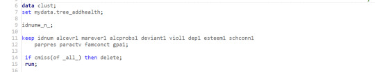
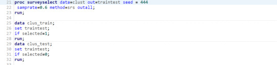
2- Dataheet split into test (40%) and training data (60%) using simple random sampling.

3- Variable standarization so the solution is not outweight by the variables measured in large scales. Limit variable standar desviation to 1 and the mean to 0.

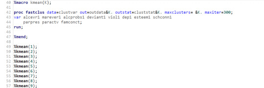
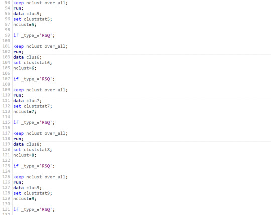
4- Define to run the code for different number of clusters.

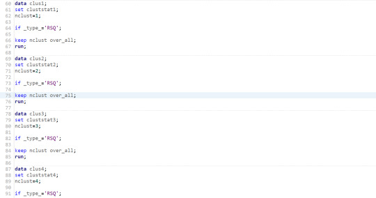
5-Extract the r-square value of each cluster to decide how many clusters are we going to consider in the analysis.

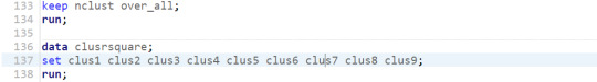
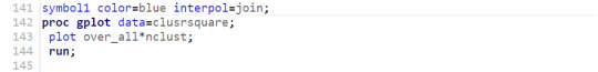
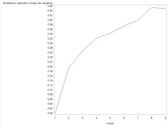
6- Plot the graphic with all the r-square values together. We are looking for an elbow in the graphic where adding cluster stop increasing the r-square value too much. Candiades (As shown in image are) k=2, K=4 and K=8

7- We further examine the solutions for the numbers of cluster suggested in previous step. For that, we use Canonical Discrimination Analysis to reduce the number of variables in order to plot them.

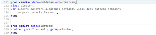
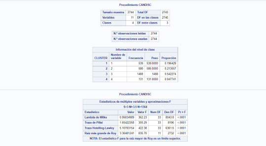
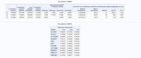
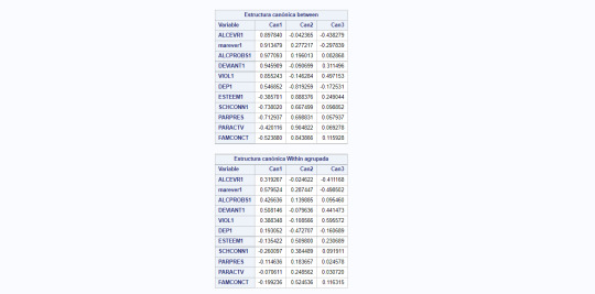
8- The following images shows the results of the canonical discrimination analysis for cluster k=4.

9- We plot the result of the analysis for cluster 4:

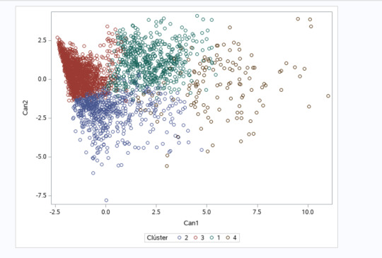
10 - In the final part the comparte the GPA values between the clusters.

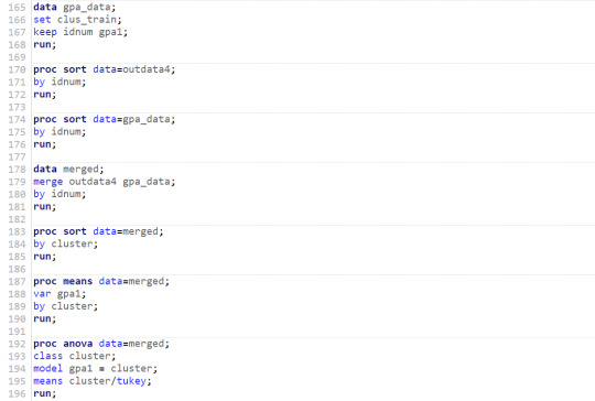
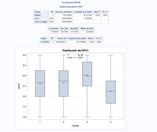
11- We can clearly trace the GPA value of each cluster to the plot in step 9. Largest GPA corresponds to cluster 3 while the smallest one goes for cluster 4.

[ml-for-data-analysis]

Lasso Regression

Week 3 exercise is about LASSO Regression. LASSO stands for Least Absolute Selection Shrinkage Operator. It is a supervised machine learning algorithm used to reduce the model overfitting. LASSO uses the causes some of the Absolute Shrinkage and Selection Operator to reduce some of the regression coefficients of the explanatory variables to zero (0) and picks the most important ones associated to the response variable.

1- The following code is run in SAS to identify the most significant subset of variables in frequent smoking cases.

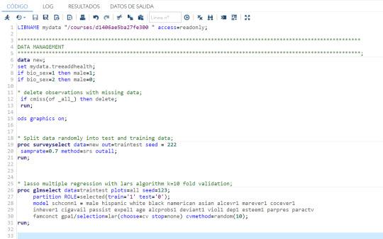
2- The next image shows the summary of the code execution. It shows the chosen dependent variable (SCHCONN1), the used selection method (LAR) and the validation criteria (Cross-validation). It also shows that 70% of the data set have been used for training while the 30% is used to test the model.

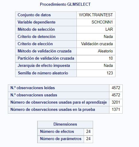
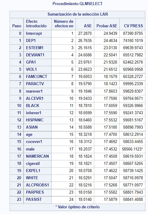
3- The most important output of the LASSO regresion is the number of variables from which the model begins to lose effectiveness. Is this case is 16, marked with and asterisk*.

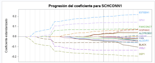
4- From the next graph, we can infer that DEP1, the light green line, had the largest regression coefficient and was entered into the model first. At second ESTEEM1, the light blue line entered into the model.

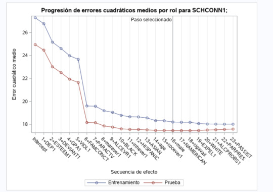
5- The last image shows that the error begins to decrease much more slowly from the seventh variable, although the optimum is 16. The fact that the MSE training data is very similar to the MSE test data implies that the prediction is quite stable for the datasets.

[ml-for-data-analysis]

Random Forest

The second week assignment deals with Random Forests. While Decision Trees are easy to visualize and interpret, they hey are not very reproducible for future data.

Random forest is a supervised machine learning model. Like Decision Trees, random forest can be use to predict continuous and categorical variable. The main difference is that Random Forest grow many trees based on different random subset of explanatory variables. Ths allows for a data driven exploration of many explanatory variables in predicting a response or target variable.

A random sample of observation is selected through a process called bagging. Each of the trees are grown on a different randomly selected sample of bagged data and the remaining unbagged are used for testing the trees.

1- The following image shows the code for generating the Random Forest in SAS studio.

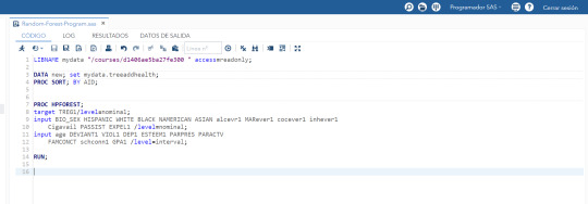
2- The bag of variables is divided between categorical variables (Nominal-->Yes/No) or quantitative variables (Interval).

3- The results of the code shows:

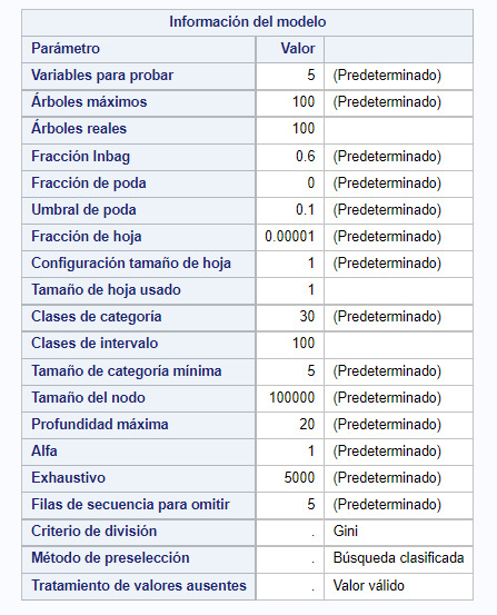
3.1-The information about the Random Forest model:

-Number of variables in each subset used to build every tree (5).

-Number of Decision Trees growth (100).

-Percentage of data to grow each tree (0.6--> 60%)

-Split criteria for the forest (Gini)

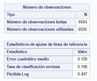
4- Observations and errors

Subsequently, the results of the generation are shown where it is seen that almost all the data of the training sample have been used 6500 of 6504.

In addition, the results shows that there have been a failure rate of 0.198.

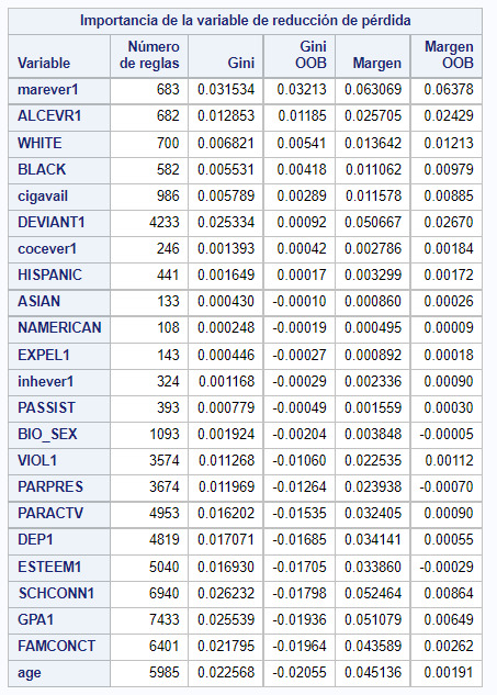
5- Finally, one of the most important outputs of the Random Forest is shown, which is which of the variables has the greatest impact on the generation of the model.

[ml-for-data-analysis]

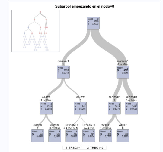
In this assignment I run decision tree to predict when someone has high risk of smoking. The decision tree selects from among a large number of variables those and their interactions that are most important in predicting the target or response variable. By applying a series of simple rules or criteria over and over again, it chooses the variable constellations that best predict the target variable (response).

The decision tree given here is called classification tree, since the response variable is categorical (Two levels).

----------------------------------

Firstly, the required dataset is loaded

We select the "AID" column as target variable, and define the rest of response variables in the model.

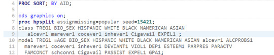
Last, we grow the tree using the "entropy" method and prune using "costcomplexity" to better adjust the trade-off of the tree complexity with the expected error.

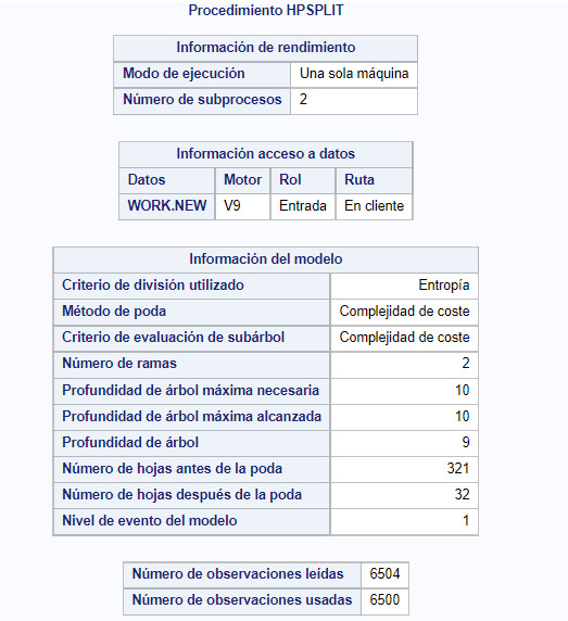
The results shows that the final tree has 10 nodes and 32 leaves.

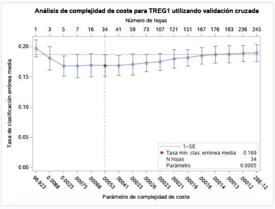
On the next picture we can see the trade-off of the pruning process to finally chose the number of nodes.

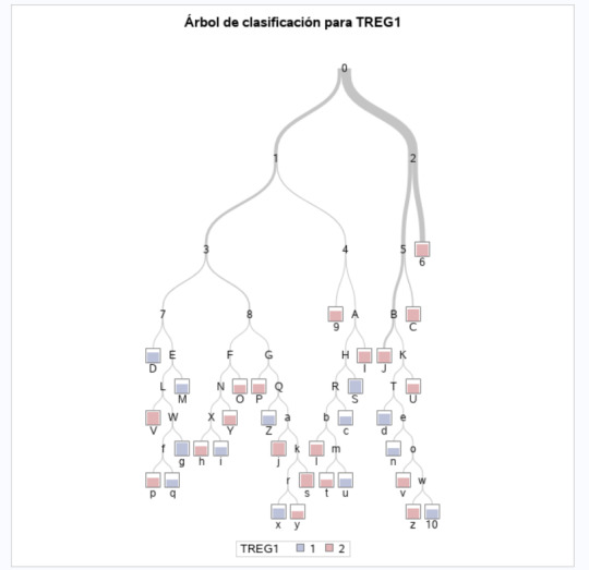
The created decision tree is shown in the next picture: