myjorry827

[myjorry827]

K-means Clustering

My codes are as follows:

from pandas import Series, DataFrame import pandas as pd import numpy as np import matplotlib.pylab as plt from sklearn.cross_validation import train_test_split from sklearn import preprocessing from sklearn.cluster import KMeans

""" Data Management """ data = pd.read_csv("tree_addhealth.csv")

#upper-case all DataFrame column names data.columns = map(str.upper, data.columns)

# Data Management

data_clean = data.dropna()

# subset clustering variables cluster=data_clean[['ALCEVR1','MAREVER1','ALCPROBS1','DEVIANT1','VIOL1', 'DEP1','ESTEEM1','SCHCONN1','PARACTV', 'PARPRES','FAMCONCT']] cluster.describe()

# standardize clustering variables to have mean=0 and sd=1 clustervar=cluster.copy() clustervar['ALCEVR1']=preprocessing.scale(clustervar['ALCEVR1'].astype('float64')) clustervar['ALCPROBS1']=preprocessing.scale(clustervar['ALCPROBS1'].astype('float64')) clustervar['MAREVER1']=preprocessing.scale(clustervar['MAREVER1'].astype('float64')) clustervar['DEP1']=preprocessing.scale(clustervar['DEP1'].astype('float64')) clustervar['ESTEEM1']=preprocessing.scale(clustervar['ESTEEM1'].astype('float64')) clustervar['VIOL1']=preprocessing.scale(clustervar['VIOL1'].astype('float64')) clustervar['DEVIANT1']=preprocessing.scale(clustervar['DEVIANT1'].astype('float64')) clustervar['FAMCONCT']=preprocessing.scale(clustervar['FAMCONCT'].astype('float64')) clustervar['SCHCONN1']=preprocessing.scale(clustervar['SCHCONN1'].astype('float64')) clustervar['PARACTV']=preprocessing.scale(clustervar['PARACTV'].astype('float64')) clustervar['PARPRES']=preprocessing.scale(clustervar['PARPRES'].astype('float64'))

# split data into train and test sets clus_train, clus_test = train_test_split(clustervar, test_size=.3, random_state=123)

# k-means cluster analysis for 1-9 clusters                                                           from scipy.spatial.distance import cdist clusters=range(1,10) meandist=[]

for k in clusters:    model=KMeans(n_clusters=k)    model.fit(clus_train)    clusassign=model.predict(clus_train)    meandist.append(sum(np.min(cdist(clus_train, model.cluster_centers_, 'euclidean'), axis=1))    / clus_train.shape[0])

""" Plot average distance from observations from the cluster centroid to use the Elbow Method to identify number of clusters to choose """

plt.plot(clusters, meandist) plt.xlabel('Number of clusters') plt.ylabel('Average distance') plt.title('Selecting k with the Elbow Method')

# Interpret 4 cluster solution model3=KMeans(n_clusters=4) model3.fit(clus_train) clusassign=model3.predict(clus_train) # plot clusters

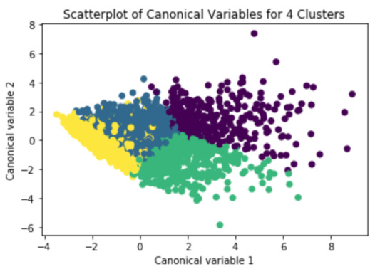
from sklearn.decomposition import PCA pca_2 = PCA(2) plot_columns = pca_2.fit_transform(clus_train) plt.scatter(x=plot_columns[:,0], y=plot_columns[:,1], c=model3.labels_,) plt.xlabel('Canonical variable 1') plt.ylabel('Canonical variable 2') plt.title('Scatterplot of Canonical Variables for 4 Clusters') plt.show()

""" BEGIN multiple steps to merge cluster assignment with clustering variables to examine cluster variable means by cluster """ # create a unique identifier variable from the index for the # cluster training data to merge with the cluster assignment variable clus_train.reset_index(level=0, inplace=True) # create a list that has the new index variable cluslist=list(clus_train['index']) # create a list of cluster assignments labels=list(model3.labels_) # combine index variable list with cluster assignment list into a dictionary newlist=dict(zip(cluslist, labels)) newlist # convert newlist dictionary to a dataframe newclus=DataFrame.from_dict(newlist, orient='index') newclus # rename the cluster assignment column newclus.columns = ['cluster']

# now do the same for the cluster assignment variable # create a unique identifier variable from the index for the # cluster assignment dataframe # to merge with cluster training data newclus.reset_index(level=0, inplace=True) # merge the cluster assignment dataframe with the cluster training variable dataframe # by the index variable merged_train=pd.merge(clus_train, newclus, on='index') merged_train.head(n=100) # cluster frequencies merged_train.cluster.value_counts()

""" END multiple steps to merge cluster assignment with clustering variables to examine cluster variable means by cluster """

# FINALLY calculate clustering variable means by cluster clustergrp = merged_train.groupby('cluster').mean() print ("Clustering variable means by cluster") print(clustergrp)

# validate clusters in training data by examining cluster differences in GPA using ANOVA # first have to merge GPA with clustering variables and cluster assignment data gpa_data=data_clean['GPA1'] # split GPA data into train and test sets gpa_train, gpa_test = train_test_split(gpa_data, test_size=.3, random_state=123) gpa_train1=pd.DataFrame(gpa_train) gpa_train1.reset_index(level=0, inplace=True) merged_train_all=pd.merge(gpa_train1, merged_train, on='index') sub1 = merged_train_all[['GPA1', 'cluster']].dropna()

import statsmodels.formula.api as smf import statsmodels.stats.multicomp as multi

gpamod = smf.ols(formula='GPA1 ~ C(cluster)', data=sub1).fit() print (gpamod.summary())

print ('means for GPA by cluster') m1= sub1.groupby('cluster').mean() print (m1)

print ('standard deviations for GPA by cluster') m2= sub1.groupby('cluster').std() print (m2)

mc1 = multi.MultiComparison(sub1['GPA1'], sub1['cluster']) res1 = mc1.tukeyhsd() print(res1.summary())

Summary:

A k-means cluster analysis was conducted to identify underlying subgroups of adolescents based on their similarity of responses on 11 variables that represent characteristics that could have an impact on school achievement. Clustering variables included two binary variables measuring whether or not the adolescent had ever used alcohol or marijuana, as well as quantitative variables measuring alcohol problems, a scale measuring engaging in deviant behaviors (such as vandalism, other property damage, lying, stealing, running away, driving without permission, selling drugs, and skipping school), and scales measuring violence, depression, self-esteem, parental presence, parental activities, family connectedness, and school connectedness. All clustering variables were standardized to have a mean of 0 and a standard deviation of 1.

Data were randomly split into a training set that included 70% of the observations (N=3201) and a test set that included 30% of the observations (N=1701). A series of k-means cluster analyses were conducted on the training data specifying k=1-9 clusters, using Euclidean distance. The variance in the clustering variables that was accounted for by the clusters (r-square) was plotted for each of the nine cluster solutions in an elbow curve to provide guidance for choosing the number of clusters to interpret.  

Figure 1. Elbow curve of average distance values for the nine cluster solutions

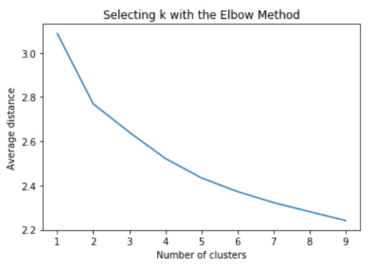
The elbow curve was inconclusive, suggesting that the 2, 3 and 4-cluster solutions might be interpreted. The results below are for an interpretation of the 4-cluster solution.  

Canonical discriminant analyses was used to reduce the 11 clustering variable down a few variables that accounted for most of the variance in the clustering variables. A scatterplot of the first two canonical variables by cluster (Figure 2 shown below) indicated that the observations in 2 clusters (purple and green) were densely packed with relatively low within cluster variance, and did not overlap very much with the other clusters.  Observations in the purple cluster  were spread out more than the other clusters, showing high within cluster variance. But, the observations in the yellow and blue clusters overlap very much with each others. The results of this plot suggest that the best cluster solution may have fewer than 4 clusters, so it will be especially important to also evaluate the cluster solutions with fewer than 4 clusters.  

Figure 2. Plot of the first two canonical variables for the clustering variables by cluster.  

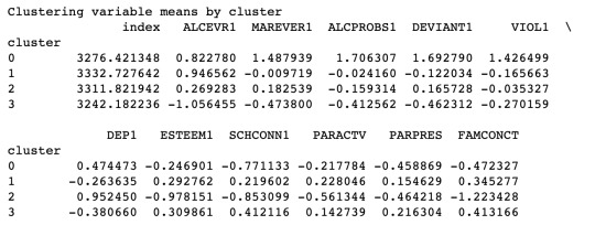
The mean values for each variables for different clusters. We could observe the differences due to the above graph.

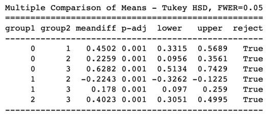
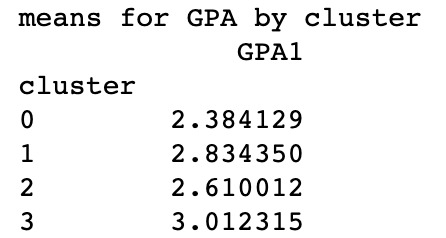
In order to externally validate the clusters, an Analysis of Variance (ANOVA) was conducting to test for significant differences between the clusters on grade point average (GPA). Results indicated significant differences between each of the clusters. A tukey test was used for post hoc comparisons between the clusters. The tukey post hoc comparisons showed significant differences between each of all the clusters on GPA.  Adolescents in cluster 3 had the highest GPA (mean=3.01), and cluster 0 had the lowest GPA (mean=2.38).

[myjorry827]

Lasso Regression

My codes are as follows:

#from pandas import Series, DataFrame import pandas as pd import numpy as np import matplotlib.pylab as plt from sklearn.model_selection import train_test_split from sklearn.linear_model import LassoLarsCV

#Load the dataset data = pd.read_csv("tree_addhealth.csv")

#upper-case all DataFrame column names data.columns = map(str.upper, data.columns)

# Data Management data_clean = data.dropna() recode1 = {1:1, 2:0} data_clean['MALE']= data_clean['BIO_SEX'].map(recode1)

#select predictor variables and target variable as separate data sets   predvar= data_clean[['MALE','HISPANIC','WHITE','BLACK','NAMERICAN','ASIAN', 'AGE','ALCEVR1','ALCPROBS1','MAREVER1','COCEVER1','INHEVER1','CIGAVAIL','DEP1', 'ESTEEM1','VIOL1','PASSIST','DEVIANT1','GPA1','EXPEL1','FAMCONCT','PARACTV', 'PARPRES']]

target = data_clean.SCHCONN1

# standardize predictors to have mean=0 and sd=1 predictors=predvar.copy() from sklearn import preprocessing predictors['MALE']=preprocessing.scale(predictors['MALE'].astype('float64')) predictors['HISPANIC']=preprocessing.scale(predictors['HISPANIC'].astype('float64')) predictors['WHITE']=preprocessing.scale(predictors['WHITE'].astype('float64')) predictors['NAMERICAN']=preprocessing.scale(predictors['NAMERICAN'].astype('float64')) predictors['ASIAN']=preprocessing.scale(predictors['ASIAN'].astype('float64')) predictors['AGE']=preprocessing.scale(predictors['AGE'].astype('float64')) predictors['ALCEVR1']=preprocessing.scale(predictors['ALCEVR1'].astype('float64')) predictors['ALCPROBS1']=preprocessing.scale(predictors['ALCPROBS1'].astype('float64')) predictors['MAREVER1']=preprocessing.scale(predictors['MAREVER1'].astype('float64')) predictors['COCEVER1']=preprocessing.scale(predictors['COCEVER1'].astype('float64')) predictors['INHEVER1']=preprocessing.scale(predictors['INHEVER1'].astype('float64')) predictors['CIGAVAIL']=preprocessing.scale(predictors['CIGAVAIL'].astype('float64')) predictors['DEP1']=preprocessing.scale(predictors['DEP1'].astype('float64')) predictors['ESTEEM1']=preprocessing.scale(predictors['ESTEEM1'].astype('float64')) predictors['VIOL1']=preprocessing.scale(predictors['VIOL1'].astype('float64')) predictors['PASSIST']=preprocessing.scale(predictors['PASSIST'].astype('float64')) predictors['DEVIANT1']=preprocessing.scale(predictors['DEVIANT1'].astype('float64')) predictors['GPA1']=preprocessing.scale(predictors['GPA1'].astype('float64')) predictors['EXPEL1']=preprocessing.scale(predictors['EXPEL1'].astype('float64')) predictors['FAMCONCT']=preprocessing.scale(predictors['FAMCONCT'].astype('float64')) predictors['PARACTV']=preprocessing.scale(predictors['PARACTV'].astype('float64')) predictors['PARPRES']=preprocessing.scale(predictors['PARPRES'].astype('float64'))

# split data into train and test sets pred_train, pred_test, tar_train, tar_test = train_test_split(predictors, target,                                                              test_size=.3, random_state=123)

# specify the lasso regression model model=LassoLarsCV(cv=10, precompute=False).fit(pred_train,tar_train)

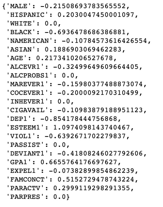
# print variable names and regression coefficients dict(zip(predictors.columns, model.coef_))

# plot coefficient progression m_log_alphas = -np.log10(model.alphas_) ax = plt.gca() plt.plot(m_log_alphas, model.coef_path_.T) plt.axvline(-np.log10(model.alpha_), linestyle='--', color='k',            label='alpha CV') plt.ylabel('Regression Coefficients') plt.xlabel('-log(alpha)') plt.title('Regression Coefficients Progression for Lasso Paths')

# plot mean square error for each fold m_log_alphascv = -np.log10(model.cv_alphas_) plt.figure() plt.plot(m_log_alphascv, model.mse_path_, ':') plt.plot(m_log_alphascv, model.mse_path_.mean(axis=-1), 'k',         label='Average across the folds', linewidth=2) plt.axvline(-np.log10(model.alpha_), linestyle='--', color='k',            label='alpha CV') plt.legend() plt.xlabel('-log(alpha)') plt.ylabel('Mean squared error') plt.title('Mean squared error on each fold')

# MSE from training and test data from sklearn.metrics import mean_squared_error train_error = mean_squared_error(tar_train, model.predict(pred_train)) test_error = mean_squared_error(tar_test, model.predict(pred_test)) print ('training data MSE') print(train_error) print ('test data MSE') print(test_error)

# R-square from training and test data rsquared_train=model.score(pred_train,tar_train) rsquared_test=model.score(pred_test,tar_test) print ('training data R-square') print(rsquared_train) print ('test data R-square') print(rsquared_test)

And the followings figures are my output plotting for coefficient progression (describe how the changes in -log(lambda) influence the coefficients for all the predictors) and mean square errors on each folders (10 folders here, describe how the changes in -log(lambda) influence the MSEs on each folders in Cross-Validation) respectively.

We observe that when lambda (alpha here) is smaller, the number of variables whose coefficients are not equal to zero increases (more variables included in the formula) and the MSE for each folders decreases and vice versa.

When the best lambda which results in a smallest average MSE value in Cross-Validation is selected, the coefficients for each predictors are as follows.

And their corresponding MSEs in the training dataset and in the test dataset, also their R-square values are shown below.

Summary:

A lasso regression analysis was conducted to identify a subset of variables from a pool of 23 categorical and quantitative predictor variables that best predicted a quantitative response variable measuring school connectedness in adolescents. Categorical predictors included gender and a series of 5 binary categorical variables for race and ethnicity (Hispanic, White, Black, Native American and Asian) to improve interpretability of the selected model with fewer predictors. Binary substance use variables were measured with individual questions about whether the adolescent had ever used alcohol, marijuana, cocaine or inhalants. Additional categorical variables included the availability of cigarettes in the home, whether or not either parent was on public assistance and any experience with being expelled from school. Quantitative predictor variables include age, alcohol problems, and a measure of deviance that included such behaviors as vandalism, other property damage, lying, stealing, running away, driving without permission, selling drugs, and skipping school. Another scale for violence, one for depression, and others measuring self-esteem, parental presence, parental activities, family connectedness and grade point average were also included. All predictor variables were standardized to have a mean of zero and a standard deviation of one.

Data were randomly split into a training set that included 70% of the observations (N=3201) and a test set that included 30% of the observations (N=1701). The least angle regression algorithm with k=10 fold cross validation was used to estimate the lasso regression model in the training set, and the model was validated using the test set. The change in the cross validation average (mean) squared error at each step was used to identify the best subset of predictor variables.

Of the 23 predictor variables, 18 were retained in the selected model. During the estimation process, self-esteem and depression were most strongly associated with school connectedness, followed by engaging in violent behavior and GPA. Depression and violent behavior were negatively associated with school connectedness and self-esteem and GPA were positively associated with school connectedness. Other predictors associated with greater school connectedness included older age, Hispanic and Asian ethnicity, family connectedness, and parental involvement in activities. Other predictors associated with lower school connectedness included being male, Black and Native American ethnicity, alcohol, marijuana, and cocaine use, availability of cigarettes at home, deviant behavior, and history of  being expelled from school. These 18 variables accounted for 33.4% of the variance in the school connectedness response variable. 

[myjorry827]

Random Forests in Python

My codes are as follows:

# import some necessary packages

from pandas import Series, DataFrame import pandas as pd import numpy as np import os import matplotlib.pylab as plt from sklearn.model_selection import train_test_split from sklearn.tree import DecisionTreeClassifier from sklearn.metrics import classification_report import sklearn.metrics # Feature Importance from sklearn import datasets from sklearn.ensemble import ExtraTreesClassifier

#load the data and take a look at it

AH_data = pd.read_csv("tree_addhealth.csv") data_clean = AH_data.dropna()

data_clean.dtypes data_clean.describe()

#Split into training and testing sets

predictors = data_clean[['BIO_SEX','HISPANIC','WHITE','BLACK','NAMERICAN','ASIAN','age', 'ALCEVR1','ALCPROBS1','marever1','cocever1','inhever1','cigavail','DEP1','ESTEEM1','VIOL1', 'PASSIST','DEVIANT1','SCHCONN1','GPA1','EXPEL1','FAMCONCT','PARACTV','PARPRES']]  #here I include all the variables except the target variable TREG1

targets = data_clean.TREG1

pred_train, pred_test, tar_train, tar_test  = train_test_split(predictors, targets, test_size=.4)

pred_train.shape pred_test.shape tar_train.shape tar_test.shape

#Build model on training data from sklearn.ensemble import RandomForestClassifier

classifier=RandomForestClassifier(n_estimators=40)  #the number of trees you want to run classifier=classifier.fit(pred_train,tar_train)

predictions=classifier.predict(pred_test)

sklearn.metrics.confusion_matrix(tar_test,predictions) sklearn.metrics.accuracy_score(tar_test, predictions)

# fit an Extra Trees model to the data model = ExtraTreesClassifier() model.fit(pred_train,tar_train) # display the relative importance of each attribute List=list(model.feature_importances_) List2=['BIO_SEX','HISPANIC','WHITE','BLACK','NAMERICAN','ASIAN','age', 'ALCEVR1','ALCPROBS1','marever1','cocever1','inhever1','cigavail','DEP1','ESTEEM1','VIOL1', 'PASSIST','DEVIANT1','SCHCONN1','GPA1','EXPEL1','FAMCONCT','PARACTV','PARPRES'] final_dict={List2[i] : List[i] for i in range(len(List))} final_dict   #from the dictionary, we can directly compare the importance between different variables.

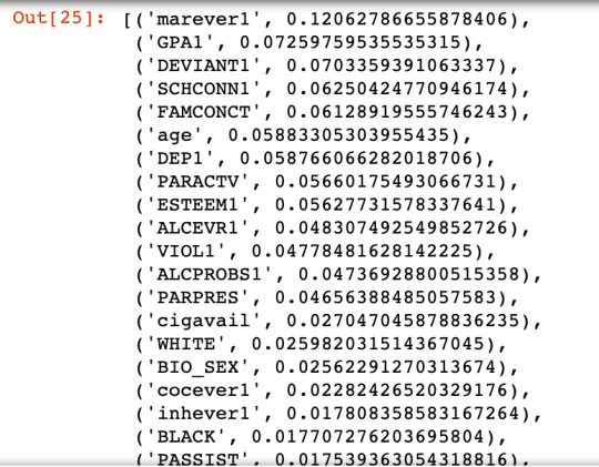
sorted(final_dict.items(), key=lambda x: x[1], reverse=True) #we can also sort them in descending order.

""" Running a different number of trees and see the effect of that on the accuracy of the prediction """

trees=range(25) accuracy=np.zeros(25)

for idx in range(len(trees)):   classifier=RandomForestClassifier(n_estimators=idx + 1)   classifier=classifier.fit(pred_train,tar_train)   predictions=classifier.predict(pred_test)   accuracy[idx]=sklearn.metrics.accuracy_score(tar_test, predictions)

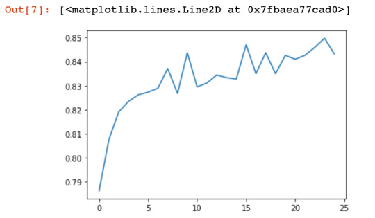
plt.cla() plt.plot(trees, accuracy) # we will see that the accuracy rate is not increasing with the number of trees we run!

Summary:

Random forest analysis was performed to evaluate the importance of a series of explanatory variables in predicting a binary, categorical response variable. The following explanatory variables were included as possible contributors to a random forest evaluating regular smoking (my response variable), age, gender, (race/ethnicity) Hispanic, White, Black, Native American and Asian. Alcohol use, marijuana use, cocaine use, inhalant use, availability of cigarettes in the home, whether or not either parent was on public assistance, any experience with being expelled from school, alcohol problems, deviance, violence, depression, self-esteem, parental presence, parental activities, family connectedness, school connectedness and grade point average.

The explanatory variables with the highest relative importance scores were  marijuana use, White ethnicity, deviance and grade point average. The accuracy of the random forest was 85%, with the subsequent growing of multiple trees rather than a single tree, adding little to the overall accuracy of the model, and suggesting that interpretation of a single decision tree may be appropriate.