nbanalytics - Tumblr blog

nbanalytics · 5 years ago

Text

Ranking the NBA Teams with a Genetic ML Algorithm

Which team is the best in the NBA? A question that most of us basketball fans think we know the answer to yet often we find it so hard to come to a consensus. In the ever-popular world of basketball analytics, I would argue that mathematical team rankings are probably the most popular and contentious problem that people try to “solve”. About two years ago I attacked this topic of debate in my very first foray into the world of basketball analytics. I was naive and inexperienced at the time, but my eventual failure led me to continue to explore the world of basketball data, statistics and machine learning…

From a math point of view there are lots of ways to approach the problem developing a computer ranking system. I will begin by establishing that the goal of any NBA ranking system should be to predict playoff success. If two teams are paired together in a playoff bracket, the higher ranked team should win more often. Additionally, the larger the difference in rating scores, the more likely the favorite team should win the playoff series. Here are a couple of simple models one might use to predict playoff success. I will use these as baseline models to which I compare my own ranking system.

The most basic way to measure team quality from the regular season is winning percentage. Below we see a plot of playoff wins versus regular season winning percentage.

There is definitely a positive and statistically significant correlation of 0.571, but can we do better? The percent of the variance in playoff success explained by regular season success alone is only 33%. Not to mention that half of the NBA champion teams fall outside of the 95% confidence interval for prediction. Obviously there are other factors that should be taken into account when predicting postseason success.

Another way to measure team quality and a popular one with computational ranking systems is average margin of victory. Below is a plot of the average margin of victory versus playoff wins.

This metric also has a positive correlation with playoff success with a statistically significant value of 0.599, which is slightly better than using regular season wins to predict playoff wins. The percent of the variance explained is also slightly better for margin of victory at 36%. However, this model also fails to include many of the champions in the 95% confidence band.

So how can be expand our ranking system to better predict postseason success? Similar to my take on measuring home court advantage, I believe that any ranking system needs to take into account the various strengths of the opponents that each teams play as well as the quality of performance in each of those games relative to an average team would against the same opponents.

From this simple criteria I developed 10 performance measures that could be included in the ranking of every team in two different categories for every game they play:

Strength of opponent

Total opponent winning percentage at time of the game

Opponent winning percentage at site of game (home/away) at time of the game

Opponent’s avg. margin of victory

Opponent’s avg. margin of victory at site of game (home/away)

Opponent’s winning percentage in last X games

Quality of play in each game compared to expected performance

Margin of victory

Over/under opponent’s points against avg.

Over/under opponent’s points for avg.

Over/under opponent’s points against avg. at site (home/away)

Over/under opponent’s points for avg. at site (home/away)

I added a few other factors to consider in the ranking algorithm as well. Overall winning percentage was included because it is a standard baseline for team rankings. Additionally, the opponent’s recent level of play could port be factored into the strength of the opponent, as well a discount factor for how long ago games were played.

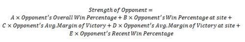
From these factors I created a linear function to combine the Strength of Opponent factors and Quality of Play factors with coefficients.

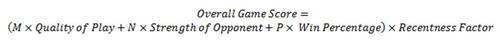
These two larger factors are then linearly combined with how recent the game was to the current point in time and the overall team winning percentage, again, with coefficients.

For a final team ranking, the score of every game is summed and the teams ordered from highest to lowest.

The value of each of these factors and how I combined them is debatable. Any ranking system is going to have some inherent subjectivity and assumptions based on the system designer and the data feed into it. The reason that I support this model is not because of the factors it takes into account, but rather that the factors can be combined in an infinite number of ways in an effort to fit the model to historical results. The theory behind the model is that the coefficients will shed light into what actually matters in winning basketball games. If defense is more important than offense the the coefficient X with be fit to be larger than the coefficient W. If performance on the road or performance at home matters, then the site specific coefficients with be large and they will be close to zero if site-specific performance is irrelevant.

This raises the question of how to best train the coefficients on historical data. At the time that I did this study, I had zero training in machine learning, so I hacked together an algorithm of my own creation that would generate random starting coefficients and search through the infinitely sized set of coefficients looking for the most predictive set. I was inspired by nature’s own machine learning technique and used breeding, mutation and natural selection to move through the coefficient search space.

The steps of the genetic algorithm were as follows:

I populated a number of “parent” sets of coefficients. I used my basketball knowledge to create coefficients I assumed would be near the optimal values for some of the parents, but randomly generated others so that my population would attack the problem from multiple “perspectives” as my intuition is not necessary what is best.

The parent sets were then “breed” with each other, two at a time, to create a large population of “children.” Each child received half of the coefficients from two different parents.

Each coefficient for every child was given the opportunity to “mutate” into a value other than that of the child’s parents.

Each child set of coefficients was then used to calculate the end of season ranking for every playoff team during the 2002-2003 through 2011-2012 NBA seasons. These rankings were used to see if the children accurately predicted the winner of each of the 150 different playoff series that occurred during those ten seasons with extra weight given to predicting the eventual champion.

The top 10 most predictive children sets were “naturally selected” to be the parent sets for the next “generation” of the algorithm.

The algorithm stopped when it accurately predicts all 10 NBA champions or reaches a pre-specified maximum number of generations.

After creating the algorithm I sat back and let it run for a while to see what kind of results would pop out. It was good to see that my “expertly” chosen coefficients accurately predicted the result of most playoff series but the algorithm quickly found a better combination. In general, the the algorithm asymptotes very quickly just above 70% prediction accuracy for all playoff series. However after just a few generations, it struggles to improve itself and never seems to predict more than 4 out of the 10 championship teams before the start of the playoffs, but it does predict 8 out of the 10 winners given the Finals match-up.

More importantly it appears that the set of coefficients that produce relatively high accuracy has many local maxima, as very different sets of coefficients produce very similar accuracy results. It was interesting to see these various formulas that my genetic algorithm converged on. Perhaps this sheds some light into being able to forecast post-season success. Either some playoff series are easy to predict (this makes sense for first round match-ups, but not for later rounds) or there are many ways to create quality teams. To avoid getting stuck at the first local maxima encountered, the algorithm allows for every child to have a random mutation that differs from either of the parents. Just as in nature this allows for innovation and diversification of the population. Along these same lines, one of the keys for arriving at the best model in light of many local maxima is to have a suitably large population to breed from. The more parents in the population, the more diverse the population, and the more opportunity the algorithm has of finding the true most-predictive model.

I investigated the impact of having a larger population, in spite of the extra computation time, by increasing the parent population size and the number of children produced each generation. As an example, here is a plot of the progression of the model over each generation with a population of 100, rather than the 10 shown above.

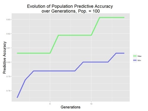
The variance in the population of models accuracy increases any time the population size is increased. It also takes more generations for the population to converge toward a homogeneous level of accuracy. More importantly, changing the population size does not increase the models ability to converge to a global optima as the total accuracy does not change much for any population size of at least 10. It was disappointing that the model very quickly reaches its most optimum set of coefficients regardless of the model parameters.

I after investigating the effect of changing the population and it’s effect on convergence, I ran the model one last time and the genetic algorithm found the most predictive model. Here is the final rankings of the model compared to the baseline models’ rankings for the 2012-2013 season.

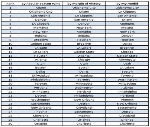
Overall the rankings of all three are pretty similar. This is not too surprising given that my model is linear combinations of values that are for the most part derived from winning percentage and margin of victory. The teams with the largest changes in my ranking from the baseline rankings are either teams that were doing much better or much worse in their most recent games. So this is how the teams fall into order during regular season, but does it translate into playoff prediction?

Here are the predictions for the 2013 NBA playoffs for he three models along side what actually went down….

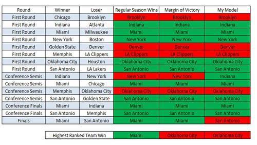
In this particular season, my model is no better than the simple predictive models based on regular season wins and regular season margin of victory. Only the wins model was able to predict the champion by ranking Miami first before the start of the playoffs. However, the goal is not to have the highest accuracy in a single season but have the model generalize to be the most predictive in any future season. Here is how the my ranking model predicts the results over the ten seasons to which the model was fit. The assumption of a linear relationship was used just as with the baseline models earlier.

My ranking system scales each team’s score to fall between 0 and 100 where the 30th ranked team has a score of 0 and the top ranked team a score of 100. As expected this team score is positively correlated with playoff success with a statistically significant value of 0.525. This is unfortunately worse than the baseline models despite being the model that the genetic algorithm found to be most predictive of postseason success. The percent of the variance explained is also worse at only 28%. But, it turns out that the team’s score it not the best metric from my ranking system for predicting playoff success because team scores are scaled based on the teams’ stats for that season. So scores can not be accurately compared with one another across seasons, and it is more realistic to predict playoff success based on the teams’ rank for that season.

This performs better, as expected, but it is still worse than the baseline models of regular season wins and regular season margin of victory. The correlation is only 0.553 and the percent of variance explained only 31%.

In light of these results, there are certainly areas where this model could be improved. Because of computation time, many of the algorithm iterations were done with too small a population and converged on local optima too soon. I did not play with any of the parameters around the randomization of the coefficients to mutate or how the parents that were “mated” were chosen. I suspect that there are ways to create population clusters or engineer other algorithm features to make the genetic algorithm converge on the best optima quicker. However, the real problem with the model has to do with the choice of a genetic algorithm to begin with.

If I were to re-do this analysis with my skill set today, I would use a different method to optimize the linear model coefficients. Ordinary least squares optimization would converge more quickly to the best-fit coefficient values, but it unclear how to set up the data set to accommodate this method and a squared error penalization may not be the best assumption in this situation. Another option would be to use an expectation maximization algorithm to converge the parameters to the best fit values from my initial assumption values. This would be an interesting experiment and is more similar to my original concept. Of course, something more powerful such as Random Forests or Neural Networks could prove more accurate with enough input information, but these methods are not for fitting parameters to an assumed model structure, but rather black-box model generators that sacrifice model interpretability. My choice of a genetic algorithm was driven by personal curiosity, and as a novice in machine learning I was unaware of what tool would be best suited to the task.

One last way to improve model would be to include more information such as, number of days rest, injuries and how types of teams match-up with one another.

In conclusion, it seems noble in the scientific sense to try and put a formula of the results of the NBA playoffs and be able to measure the quality of a basketball team, but the truth is really the old cliché, basketball games and trophies aren’t won on paper, but rather, on the hardwood. I learned a few analytics lessons. More complex models are not guaranteed be better than the simpler models they hope to improve upon, and any data scientist needs to know when to use the right model for the given problem. While I never expected a genetic algorithm to be the best way to fit my model, it turns out that it was never properly suited to the task given my evaluation measure and the computation time involved.

As fan of the port I have come to realize that this is actually an encouraging result. It should not be easy to change conventional wisdom or predict the future. I am glad that there is the white noise randomness of blown charging calls and streak-shooting that make each game dramatic and exciting. Sure there are better measures of the true quality of a team beyond winning percentage or margin of victory, but if we knew with any certainty the outcome of a basketball, why would we even bother to watch?

This analysis was done in Matlab and the results processed in a combination of Matlab and R.

All of the data was courtesy of basketball-reference.com

More general information about genetic algorithms can be found at http://en.wikipedia.org/wiki/Genetic_algorithm

Other computer ranking systems for NBA teams can be found at:

http://www.usatoday.com/sports/nba/sagarin/

http://www.teamrankings.com/nba/ranking/overall-power-ranking-by-team

http://espn.go.com/nba/hollinger/powerrankings

Feb 7

Facebook

Twitter

Google

Tumblr

Random post

Browse the Archive

Get the RSS

About

What started out at a hobby trying to separate basketball facts from opinion has led me to a career in data analytics. Perhaps I should share some of my mathematical musings...

Ask me anything

Connect

0 notes

nbanalytics · 5 years ago

Text

success

fail

Feb MAR Apr 23 2018 2019 2020

26 captures

21 Jan 2016 - 27 Sep 2019

About this capture

COLLECTED BY

Organization: Alexa Crawls

Starting in 1996, Alexa Internet has been donating their crawl data to the Internet Archive. Flowing in every day, these data are added to the Wayback Machine after an embargo period.

Collection: Alexa Crawls

Starting in 1996, Alexa Internet has been donating their crawl data to the Internet Archive. Flowing in every day, these data are added to the Wayback Machine after an embargo period.

TIMESTAMPS

__wm.bt(625,27,25,2,"web","http://nbanalytics.tumblr.com/","20190323161114",1996,"/_static/",["/_static/css/banner-styles.css?v=HyR5oymJ","/_static/css/iconochive.css?v=qtvMKcIJ"]); NBAnalyticsfigure{margin:0}.tmblr-iframe{position:absolute}.tmblr-iframe.hide{display:none}.tmblr-iframe--amp-cta-button{visibility:hidden;position:fixed;bottom:10px;left:50%;transform:translateX(-50%);z-index:100}.tmblr-iframe--amp-cta-button.tmblr-iframe--loaded{visibility:visible;animation:iframe-app-cta-transition .2s ease-out} /* If this option is selected, the theme will use a solid background instead of an image */ body { background: #000000 url(http://web.archive.org/web/20190323161114im_/http://static.tumblr.com/06e5dcbee1eebcb1fc08923a0dbbdf9e/deauzpq/9Mumzs7m4/tumblr_static_maxresdefault.jpg) fixed top left; } /* If this option is selected, the theme will use a solid background instead of an image */ var enableAudiostream = false; var audioplayerTagFilter = false; var enableDisqus = false; var enableTwitter = false; var enableFlickr = false; var enableInstagram = false; var totalBlogPages = '1'; {"@type":"ItemList","url":"http:\/\/web.archive.org\/web\/20190323161114\/http:\/\/nbanalytics.tumblr.com","itemListElement":[{"@type":"ListItem","position":1,"url":"http:\/\/web.archive.org\/web\/20190323161114\/http:\/\/nbanalytics.tumblr.com\/post\/75952859870\/ranking-the-nba-teams-with-a-genetic-ml-algorithm"},{"@type":"ListItem","position":2,"url":"http:\/\/web.archive.org\/web\/20190323161114\/http:\/\/nbanalytics.tumblr.com\/post\/74366758922\/what-team-benefits-the-most-from-home-cooking"}],"@context":"http:\/\/web.archive.org\/web\/20190323161114\/http:\/\/schema.org"}

Now Playing Tracks

NBAnalytics

Facebook

Twitter

Google

Tumblr

Ranking the NBA Teams with a Genetic ML Algorithm

The most basic way to measure team quality from the regular season is winning percentage. Below we see a plot of playoff wins versus regular season winning percentage.

Another way to measure team quality and a popular one with computational ranking systems is average margin of victory. Below is a plot of the average margin of victory versus playoff wins.

From this simple criteria I developed 10 performance measures that could be included in the ranking of every team in two different categories for every game they play:

Strength of opponent

Total opponent winning percentage at time of the game

Opponent winning percentage at site of game (home/away) at time of the game

Opponent’s avg. margin of victory

Opponent’s avg. margin of victory at site of game (home/away)

Opponent’s winning percentage in last X games

Quality of play in each game compared to expected performance

Margin of victory

Over/under opponent’s points against avg.

Over/under opponent’s points for avg.

Over/under opponent’s points against avg. at site (home/away)

Over/under opponent’s points for avg. at site (home/away)

I added a few other factors to consider in the ranking algorithm as well. Overall winning percentage was included because it is a standard baseline for team rankings. Additionally, the opponent’s recent level of play could be factored into the strength of the opponent, as well a discount factor for how long ago games were played.

From these factors I created a linear function to combine the Strength of Opponent factors and Quality of Play factors with coefficients.

These two larger factors are then linearly combined with how recent the game was to the current point in time and the overall team winning percentage, again, with coefficients.

For a final team ranking, the score of every game is summed and the teams ordered from highest to lowest.

The steps of the genetic algorithm were as follows:

The parent sets were then “breed” with each other, two at a time, to create a large population of “children.” Each child received half of the coefficients from two different parents.

Each coefficient for every child was given the opportunity to “mutate” into a value other than that of the child’s parents.

The top 10 most predictive children sets were “naturally selected” to be the parent sets for the next “generation” of the algorithm.

The algorithm stopped when it accurately predicts all 10 NBA champions or reaches a pre-specified maximum number of generations.

Here are the predictions for the 2013 NBA playoffs for he three models along side what actually went down….

One last way to improve model would be to include more information such as, number of days rest, injuries and how types of teams match-up with one another.

As fan of the sport I have come to realize that this is actually an encouraging result. It should not be easy to change conventional wisdom or predict the future. I am glad that there is the white noise randomness of blown charging calls and streak-shooting that make each game dramatic and exciting. Sure there are better measures of the true quality of a team beyond winning percentage or margin of victory, but if we knew with any certainty the outcome of a basketball, why would we even bother to watch?

This analysis was done in Matlab and the results processed in a combination of Matlab and R.

All of the data was courtesy of basketball-reference.com

More general information about genetic algorithms can be found at http://en.wikipedia.org/wiki/Genetic_algorithm

Other computer ranking systems for NBA teams can be found at:

http://www.usatoday.com/sports/nba/sagarin/

http://www.teamrankings.com/nba/ranking/overall-power-ranking-by-team

http://espn.go.com/nba/hollinger/powerrankings

Feb 7

Facebook

Twitter

Google

Tumblr

What team benefits the most from home cooking?

Basketball just like any spectator sport is subject the phenomenon we all know and love as “Home Court Advantage.” Even the casual sports fan knows that their favorite team has a better chance of winning in their home arena than they do in somebody else’s. In the NBA, the rule of thumb is that the home team tends to do about 3 points better than they would if the game were played at a neutral site. That means that there is a whopping 6 point swing depending on whose gym the game is being played in which is significant considering that the average margin of victory in the NBA is only 3.3 points.

So what is the cause of this crowd pleasing phenomenon? The standard theories include: the home crowd support, player’s sleeping in their own bed, the home game routine, and the additional rest home teams enjoy courtesy of the typical NBA season (see endnote references). I’m sure in reality that it is some combination of all of these factors, but who’s to say that all home court advantages were created equal?

Awhile ago, I spent a day investigating this very topic because the best home court advantage in the NBA is a pretty frequent subject in national TV telecasts. The media and coaches love to point to how are it is to win in places like the Pepsi Center in the mile-high altitude of Denver or beneath the raucous crowds at Oracle Arena in Oakland. So do the numbers back up these usual candidates for toughest places to play in the NBA? First, a clear definition of home court advantage needs to be established.

I care about consistent fan bases and a home court advantage that is independent of individual players or particular team rosters in a given year, so it is important to study the impact of home court advantage over a number of seasons. I chose to study all NBA games from the 2002-2003 season through the 2011-2012 season, a period of time that is long enough for NBA rosters to have completely turned over during that time frame and for most to have had both good and bad years. Also, calculating a team’s benefit from playing at home should be more sophisticated than simply subtracting each teams away margin of victory from their home margin of victory. This simple metric does not take into account the different schedules that each team plays or the imbalance in the number home vs. away games that teams play against each other (see endnote references). A team like the Houston Rockets that have 26 homes against the stronger eastern conference whereas the Toronto Raptors have only 15 home games against Western conference foes. This season at least, the Raptors play one game home and one road game against the Rockets compared to the the much weaker Orlando Magic against whom they play two home games and only one away game. Toronto’s home margin would be expect to be ballooned slightly by having an easier home schedule than road schedule since the other road game is most likely against a team of higher quality that the Magic.

Therefore, I attempted to insulate my calculation of home court advantage against the different schedules that every team experiences and the differences in schedules across NBA seasons. This is done by calculating the average points for and against for all visiting teams and then comparing that to how that team does in all of the the 30 NBA arenas. The strength of a home court advantage is based on how many more points the home team tends to win by against its opponents compared to how many points the visiting teams tend to lose by. This normalizes the home margin of victory against the strength of the visiting opponents for all teams. This value can then be compared to how well the same team does on the road to create the average benefit that each team gets from playing at home.

In essence, the best home court advantage does not belong to the team that wins the highest percentage of their home games (That was San Antonio at 72% during the 10 seasons of study). Nor is it the team that has the largest increase in home winning percentage over road winning percentage (That was Washington with over a 40% increase). It is the team whose expected point differential for home games performance increases the most in expected point differential between home games and away games relative to the average point differential of the opposing team.

As an example. Let’s study the games between Houston and Toronto from the 2012-2013 season. Houston averaged 106.0 points per game and allows 102.5 points per game for a average margin of victory of 3.5 points. Toronto averaged 97.2 points per game and allows 98.7 points per game for an average margin of victory of -1.5 points. In the first game, in Houston, the Rockets won 117-101. Toronto prevailed at home in the rematch 103-96. Assuming both of the games had been at a neutral site,we would have expected Houston to win both games by about 2.5 points (given that both teams had played teams of equal quality of course). To calculate the advantage of home court between Toronto and Houston I looked at the change in the expect value for margin of victory. Houston increased their expected margin from 2.5 to 16 for an increase of 13.5 points at home. The road margin dropped from the 2.5 expected to -7 for a -9.5 points. In this match up, home court was worth a whopping 23 points to the Houston Rockets and, via symmetry, to Toronto as well. I performed this calculation for all of the 29 head-to-head matched between teams for each season and then averaged the increases to find an average increase in margin of victory for each team over the whole season. To reduce the variation that is expected from season to season, I then average then ten seasons of study to create an estimate for the standard home court advantage expected in all 30 NBA arenas.

So now for the results of the study which is what we all want to see…

Below is a ranked chart of each team with the changes in Winning Percentage, Points For, Points Against, and Margin of Victory between home and away from the 2002-2003 to 2011-2012 seasons.

Unsurprisingly, the usual suspects rise to the top. However notice that often forgotten Utah gains the most from playing at home. I suspect this is for having an elevation only 1,000 feet lower than Denver and better than average crowd that loves their only major pro-sports team in town.

As I claim that my analyses are grounded in math and science, I must ask whether these results are statistically significant. First let’s look at a plot of the three best and three worst teams’ home advantage over the ten seasons compare to the average home court advantage that year.

While I admit that there is a lot of noise from season to season, there is a clear difference between Utah, Denver, and Golden State compared to Minnesota, Philadelphia and Boston. The former teams almost always have above average home court advantages while the latter teams almost always under perform at home.

But are these claims statistically significant? Boston’s league worst home court advantage of 4.67 is statisitically different from the assumption that home court advantage does not exist with a p-value of 2.1x10-9, a really small number. So, I conclude that home court advantage does indeed exist, as well all expected. I then looked to see whether Boston’s and Utah’s advantages were statistically different than the league average. The resulting p-values were 0.004 and 0.001 respectively, so yes Utah can be considered a more difficult environment to play in compared to Boston, given the quality of the teams are the same. But the question we all care about is: Can we definitely say that Utah has the greatest home court advantage in the NBA? Namely, is the Jazz’s league lead 9.3 point advantage better than Denver’s 8.8 point advantage?

Well, we can not really make such a claim, as the p-value for the hypothesis test to whether Utah’s average home court advantage is greater than Denver’s is a rather large 0.37. In fact, I had to go all the way down to Sacramento with the sixth best advantage to be able to even claim that Utah has a significant advantage over the King’s with even a 90% confidence level. Essentially, all of the usual suspects can make an argument that they place is the toughest to play, and there is no clear cut winner. In reality, it probably varies year to year based on the players on the roster and other factors like rest and injuries.

In conclusion, the effect of home court advantage is real. There is a clear difference in the effect of home court across the NBA as Utah’s advantage is twice that of Boston’s. However because there is a lot of variation in relative home court advantage from season to season there is no clear “hardest place to play” in the NBA. Much of the effect of home court advantage can be clouded by the unbalanced strength of schedule in the NBA, but this can be accounted for by factoring in the opponent’s strength. It is also unclear what individual variables contribute to this phenomenon but it appears that crowd support and altitude have an effect.

I also want to point out further points of research that could be done with this data include: investigating the relationship between team record and home court advantage or whether these variables are independent, why some teams advantage is primarily on offense or defense, why the increase in winning percentage is only loosely correlated to increase in margin of victory, and investigating if home court advantage is consistently around 3.2 every year or has an identifiable trend.

This analysis was done in Matlab and the results processed in R.

All of the data was courtesy of basketball-reference.com

Below are a few links to related material:

Days Rest’s effect on Home Court Advantage-

http://www.amstat.org/chapters/boston/nessis07/presentation_material/Dylan_Small.pdf

How the NBA creates it’s schedule and the imbalances-

http://www.nbastuffer.com/component/option,com_glossary/Itemid,90/catid,44/func,view/term,How%20the%20NBA%20Schedule%20is%20Made/

Jan 23

Random post

Browse the Archive

Get the RSS

About

What started out at a hobby trying to separate basketball facts from opinion has led me to a career in data analytics. Perhaps I should share some of my mathematical musings...

Ask me anything

Connect

tumblrNotesInserted = function(notes_html) { $('.notes .note:not(.processed) img').each(function(i){ var note = $(this).parent().parent(); var avaurl = $(this).attr("src"); avaurl = avaurl.replace('16.gif','64.gif'); avaurl = avaurl.replace('16.png','64.png'); avaurl = avaurl.replace('16.jpg','64.jpg'); $(this).attr('src', avaurl).parent().addClass('avatar-wrap'); note.append($('<span class="ir note-glyph">')).addClass('processed'); }); $('.more_notes_link').prepend($('<div>',{'class':'more-notes-icon'})); } var _gaq=[['_setAccount','UA-43477248-2'],['_trackPageview']]; (function(d,t){var g=d.createElement(t),s=d.getElementsByTagName(t)[0]; g.src=('https:'==location.protocol?'//web.archive.org/web/20190323161114/http://ssl':'//web.archive.org/web/20190323161114/http://www')+'.google-analytics.com/ga.js'; s.parentNode.insertBefore(g,s)}(document,'script')); var themeTitle = "Fluid Neue Theme"; var url = "http://web.archive.org/web/20190323161114/http://fluid-theme.pixelunion.net"; (function() { var pxu = document.createElement('script'); pxu.type = 'text/javascript'; pxu.async = true; pxu.src = 'http://web.archive.org/web/20190323161114/http://cdn.pixelunion.net/customize/pxucm.js'; var isCustomize = (window.location.href.indexOf('/customize_preview_receiver.html') >= 0) ? true: false; var isDemo = (window.location.href.indexOf(url) >= 0) ? true: false; (isCustomize || isDemo) && ((document.getElementsByTagName('head')[0] || document.getElementsByTagName('body')[0]).appendChild(pxu)); })(); var pxuConversionLabel = "ex5HCJmipgIQ58Wg4gM"; var pxuDemoURL = "fluid-theme.pixelunion.net"; var pxuIsDemo = (window.location.href.indexOf(pxuDemoURL) != -1); var pxuTriggerConversion = (document.referrer.indexOf(pxuConversionLabel) != -1); if (pxuTriggerConversion && !pxuIsDemo) { /* <![CDATA[ */ var google_conversion_id = 1011360487; var google_conversion_language = "en"; var google_conversion_format = "3"; var google_conversion_color = "ffffff"; var google_conversion_label = pxuConversionLabel; var google_conversion_value = 40; /* ]]> */ }

0 notes