notstatschat

[notstatschat]

We’ve moved

Nothing’s going to change here, but new entries and a copy of almost everything from here is at netlify 

[notstatschat]

Graduation

So, I gave one of the graduation addresses during Silly Hat Week last week.  It’s not my usual style of writing, but since there’s no point being embarrassed about a speech you’ve already given in front of your boss, your boss’s boss, and 2000 other people, I thought I’d post it here. 

Chancellor, Vice-Chancellor, Members of Council, fellow Members of the University, Graduands, families and friends: kia ora tātou

It’s five o’clock on a Friday. In the cultural traditions of my people, that’s a time to celebrate the successful end of some hard work. Today we're celebrating a longer period of harder work than most Fridays, and with two thousand more people than usual.

For some of you, the journey will have been especially challenging: your friends didn't go to university with you, or you've had to juggle family and work and study obligations, or you're studying in a foreign country and a foreign language. But it won't have been easy for anyone: your degree is a real achievement to be proud of.

Congratulations, graduands. You did it.

In a few minutes from now, the Chancellor will say the magic words and it will be official: you know Science. I'm sure I speak for my colleagues on the stage when I say we're all proud to have helped.

Of course, no-one one knows everything about science, but you do know more than most people in New Zealand -- or in the world.  Part of that is the specific facts about plankton or neutrinos or Sonogashira couplings that you've studied. Just as important is what you've learned about how science works: how it fits together like a crossword puzzle, and how you can use what we already know about the world to test answers to new questions.

Some of you will go on to make your own contributions to scientific knowledge -- in fact, some of you already have. Many of you will use what you've learned about science in your future careers.  But I want to talk about a way all of you can use your scientific training to contribute to the community.

Today, scientific research is helping us uncover problems and risks for society and potential solutions to them: climate change, drug policy, road pricing, crime prediction, and many more.  The news media report some of this research, but tend to lose the context it was done in: they don't distinguish well between solid and speculative ideas or between major and minor risks or between breakthroughs and the usual incremental scientific advances. It's not that the journalists don't care, it's that they don't have the time and resources to cover each story in the depth it would need — it’s not sports journalism.

But the news -- and maybe social media -- is how most people get their information about policy issues and the science informing them. And that's a problem.

In a democracy we want decisions made in a way that reflects the whole range of interests and values across society. It's hard to do that unless there's a shared understanding of what the problems and potential solutions are. Either people need to understand the issues themselves or they need to trust someone else's understanding.  

Helping create this shared understanding is partly a job for those of us on the stage -- one of the University's official roles,  according to the legislation that set it up, is to act as a critic and conscience for society. Since I moved to New Zealand I've been spending a lot more time on science communication: blogging, tweeting, talking to journalists and journalism students. Many of my colleagues do the same. But there are things you can do that we can't.  

As I said at the beginning, you know more about science -- both the basic facts, and the ways of answering questions -- than most people in New Zealand, or most people in the world. Knowledge is power, and with modest power comes modest responsibility.   Each of you has the skills and training to understand at least some of the scientific issues in our political and social debates. If you have a smartphone, you've got instant access to a lot of the world's scientific knowledge in a way that was unimaginable fifty years ago. And, most importantly, you've got people -- friends and family -- who trust you to share their values and interests, when they wouldn't trust me.  

I'm not suggesting you go around preaching science to all your friends: that would just get annoying, and you'd end up with fewer friends. But if you keep up the habits of learning from your time at the University, and if you look into issues carefully before making up your mind it's going to have an influence on the people around you -- and sometimes they’ll ask your opinion.

Now, trying to follow the facts behind social issues can be uncomfortable.  Like all of us, you're going to sometimes find out that the arguments you'd like to support are wrong, or at least a lot weaker than you'd like. In fact, finding that you were wrong about something is one of the best signs that you're still doing science right.  

So, I'm going to propose a challenge: at the end of every year when you think about New Year's resolutions, also ask yourself: "What did I change my mind about this year?"

[notstatschat]

svylme

I’m working on an R package for mixed models under complex sampling.  It’s here. At the moment, it only tries to fit two-level linear mixed models to two-stage samples -- for example, if you sample schools then students within schools, and want a model with school-level random effects. Also, it’s still experimental and not really tested and may very well contain nuts.

The package uses pairwise composite likelihood, because that’s a lot easier to implement efficiently than the other approaches, and because it doesn’t have the problems with nonlinearity and weight scaling. On the downside, there’s some loss in efficiency, especially in situations where both the predictor and response are very strongly correlated within clusters. 

Currently, I’ve only got standard error estimation for the fixed effects. I think I know how to do it for the random effects, but it’s enough of a pain that I don’t want to unless people actually need it.  A resampling approach may turn out to be better. 

Extending this to more levels of model and stages of sampling shouldn’t be that hard -- more tedious than difficult -- as long as the model level are nested in the sampling stages. That is, you could have school districts as sampling units above schools, or classrooms as a model level below schools. 

The more-general case where model and sampling units aren’t nested turns out to be straightforward for estimation (though efficient implementations are non-trivial) but rather more complicated for standard error estimation.  It will come, but not right now. 

Generalised linear mixed models are also tricky: for what I’m doing now you don’t need the conditional modes of the random effects, but for efficient computation in GLMMs you do, in order to use adaptive Gaussian quadrature. It should still be feasible, but it may be a while. 

The package relies on lme4 in two ways. First, it uses lmer to get good starting values for optimisation, which is always helpful. Second, it uses Doug Bates’s idea of profiling out the fixed effects parameters and then just feeding the profile loglikelihood to a black-box, derivative-free optimiser. Profiling cuts the number of parameters down a lot, which makes optimisation easier.  Using a derivative-free optimiser simplifies the code a lot, since the derivatives with respect to the variance components get messy fast. 

[notstatschat]

Small p hacking

The proposal to change p-value thresholds from 0.05 to 0.005 won’t die. I think it’s targeting the wrong question:  many studies are too weak in various ways to provide the sort of reliable evidence they want to claim, and the choices available in analysis and publication process eat up too much of that limited information.  If you use p-values to decide what to publish, that’s your problem, and that’s what you need to fix.

One issue that doesn’t get as much attention is how a change would affect the sensitivity of p-values to analysis choices.  When we started doing genome-wide association studies, we noticed that the results were much more sensitive than we had expected. If you changed the inclusion criteria or the adjustment variables in the model, the p-value for the most significant SNPs often changed a lot.  Part of that is just having low power. Part of it is because the Normal tail probability gets small very quickly: small changes in a $Z$-statistic of -5 give you quite large changes in the tail probability. Part of it is because we were working at the edge of where the Normal approximation holds up: analyses that are equivalent to first order can start showing differences.  Overall, as Ken Rice put it “the data are very tired after getting to $5\times 10^{-8}$”, and you can’t expect them to do much additional work.  In our (large) multi-cohort GWAS we saw these problems only at very small p-values , but with smaller datasets you’d see them a lot earlier.

None of this is a problem if you have a tightly pre-specified analysis and do simulations to check that it’s going to be ok.  But it did mean we had to be more careful about being too flexible.  Fortunately, the computational load of GWAS (back then) was enough to encourage pre-specified analyses.  But if you’re trying to make a change to general statistical practice in order to mask some of the symptoms of analysis flexibility and publication bias, you do need to worry.

[notstatschat]

Chebyshev’s inequality and `UCL’

Chebyshev’s inequality (or any of the other transliterations of Чебышёв) is a simple bound on the proportion of a distribution that can be far from the mean. The Wikipedia page, on the other hand, isn’t simple. I’m hoping this will be more readable.

We have a random quantity $X$ with mean $\mu$ and variance $\sigma^2$, and -- knowing nothing else -- we want to say something about the probability that $X-\mu$ is large.  Since we know nothing else, we need to find the largest possible value of $\Pr(|X-\mu|\geq d)$ for any distribution with that mean and variance. 

It’s easier to think about the problem the other way: fix $\Pr(|X-\mu|\geq d)$, and ask how small we can make the variance.  So, how can we change the distribution to reduce the variance without changing $\Pr(|X-\mu|\geq d)$?  For any point further than $d$ away we can move it to distance $d$ away. It still has distance at least $d$, but the variance is smaller.  For any point closer than $d$ we can move it all the way to the mean. It’s still closer than $d$, and the variance is smaller.

So, the worst-case distribution has all its probability at $\mu-d$, $\mu$, or $\mu+d$.  Write $p/2$ for the probability that $X=\mu-d$. This  must be the same as the probability that $X=\mu+d$, or $\mu$ wouldn’t be the mean.  By a straightforward calculation the variance of this worst-case distribution is $\sigma^2=pd^2$.  So, $p=\sigma^2/d^2$ for the worst-case distribution, and $p\leq \sigma^2/d^2$ always.

In environmental monitoring there’s an approach to upper confidence limits for a mean based on this: the variance of the mean of $n$ observations is $\sigma^2/n$, and the probability of being more than $d$ units away from the mean is bounded by $\sigma^2/nd^2$.  The problem, where this is used in environmental monitoring, is that you don’t know $\sigma^2$.  You’ve got an estimate based on the data, but this estimate is going to be unreliable in precisely the situations where you’d need a conservative, worst-case interval.  The approach is ok if you’ve taken enough samples to see the bad bits of the pollution distribution, but it’s not very helpful if you don’t know whether you have.

[notstatschat]

Why pairwise likelihood?

Xudong Huang and I are working on fitting mixed models using pairwise composite likelihood. JNK Rao and various co-workers have done this in the past, but only for the setting where the structure (clusters, etc) in the sampling is the same as in the model.  That’s not always true. 

The example that made me interested in this was genetic analyses from the Hispanic Community Health Survey.  The survey is a multistage sample: census block groups and then households. The models have random effect structure corresponding to relatedness.  Since there are unrelated people in the same household (eg, spouses) and related people in different households, the sampling and design structures are very different.

What you’d start off trying to do in a traditional design-based approach is to estimate the population loglikelihood.  In a linear mixed model that’s of the form $$-\frac{1}{2}\log\left|\Xi\right| -\frac{1}{2} (y-\mu(\beta))^T\Xi^{-1} y-\mu(\beta))$$ for a covariance matrix $\Xi$ and regression parameters $\beta$. 

The way I’ve described the problem previously is “it’s not clear where you stick the weights”. That’s true, but it’s worth going into more detail.  Suppose you know $\Xi$ for the whole population.  You then know the log-determinant term, and the residual term is a pairwise sum. If $R_{ij}$ is the indicator that the pair $(i,\,j)$ is sampled, and $\pi_{ij}$ is the probability, you could use $$\hat\ell =-\frac{1}{2}\log\left|\Xi\right| -\frac{1}{2} \sum_{i,j} \frac{R_{ij}}{\pi_{ij}}(y-\mu(\beta))_i^T\left(\Xi^{-1}\right)_{ij} y-\mu(\beta))_j$$

Typically we don’t know $\Xi$ for the whole population: it can depend on covariates (in a random-slope model), or we might not even know the number of people in non-sampled clusters, or in the genetic example we wouldn’t know the genetic relationships between non-sampled people.  Also, the full population could be quite big, so working out $-\frac{1}{2}\log\left|\Xi\right|$ might be no fun.  The approach might be worth trying for a spatial model, but it’s not going to work for a health survey.

If the model and design structures were the same, we might treat $\Xi$ as block diagonal, with some blocks observed and others not, and hope to easily rescale the sample log determinant to the population one. But in general that will be hopeless, too. 

Pairwise composite likelihood works because we can use a different objective function, one that really is a sum that’s easy to reweight.  If $\ell_{ij}$ is the loglikelihood based on observations $i$ and $j$, then in the population $$\ell_\textrm{composite} = \sum_{i,j} \ell_{ij}$$ and based on the sample $$\hat\ell_\textrm{composite} = \sum_{i,j} \frac{R_{ij}}{\pi_{ij}}\ell_{ij}.$$ We now only need to be able to work out $\Xi$ for observed pairs of people, which we can easily do.  Since the summands are honest-to-Fisher loglikelihoods, they have their expected maximum at the true parameter values and estimation works straightforwardly for both $\beta$ and $\Xi$. Variance estimation for $\hat\beta$ doesn’t work so easily: a sandwich estimator has a lot of terms, and proving it’s consistent is fairly delicate. But it is consistent.

We would do strictly better in terms of asymptotic efficiency by going beyond pairs to triples or fourples or whatever. But even triples would up the computational complexity by a factor of $n$, and require us to have explicit formulas for sixth-order joint sampling probabilities -- and it gets exponentially worse for larger tuples. 

[notstatschat]

Faster generalised linear models in largeish data

There basically isn’t an algorithm for generalised linear models that computes the maximum likelihood estimator in a single pass over the $N$ observatons in the data. You need to iterate.  The bigglm function in the biglm package does the iteration using bounded memory, by reading in the data in chunks, and starting again at the beginning for each iteration. That works, but it can be slow, especially if the database server doesn’t communicate that fast with your R process.

There is, however, a way to cheat slightly. If we had a good starting value $\tilde\beta$, we’d only need one iteration -- and all the necessary computation for a single iteration can be done in a single database query that returns only a small amount of data.  It’s well known that if $\|\tilde\beta-\beta\|=O_p(N^{-1/2})$, the estimator resulting from one step of Newton--Raphson is fully asymptotically efficient. What’s less well known is that for simple models like glms, we only need $\|\tilde\beta-\beta\|=o_p(N^{-1/4})$.

There’s not usually much advantage in weakening the assumption that way, because in standard asymptotics for well-behaved finite-dimensional parametric models, any reasonable starting estimator will be $\sqrt{N}$-consistent. In the big-data setting, though, there’s a definite advantage: a starting estimator based on a bit more than $N^{1/2}$ observations will have error less than $N^{-1/4}$.  More concretely, if we sample $n=N^{5/9}$ observations and compute the full maximum likelihood estimator, we end up with a starting estimator $\tilde\beta$ satisfying $$\|\tilde\beta-\beta\|=O_p(n^{-1/2})=O_p(N^{-5/18})=o_p(N^{-1/4}).$$

The proof is later, because you don’t want to read it. The basic idea is doing a Taylor series expansion and showing the remainder is $O_p(\|\tilde\beta-\beta\|^2)$, not just $o_p(\|\tilde\beta-\beta\|).$

This approach should be faster than bigglm, because it only needs one and a bit iterations, and because the data stays in the database. It doesn’t scale as far as bigglm, because you need to be able to handle $n$ observations in memory, but with $N$ being a billion, $n$ is only a hundred thousand. 

The database query is fairly straightforward because the efficient score in a generalised linear model is of the form  $$\sum_{i=1}^N x_iw_i(y_i-\mu_i)$$ for some weights $w_i$. Even better, $w_i=1$ for the most common models. We do need an exponentiation function, which isn’t standard SQL, but is pretty widely supplied. 

So, how well does it work? On my ageing Macbook Air, I did a 1.7-million-record logistic regression to see if red cars are faster. More precisely, using the “passenger car/van” records from the NZ vehicle database, I fit a regression model where the outcome was being red and the predictors were vehicle mass, power, and number of seats. More powerful engines, fewer seats, and lower mass were associated with the vehicle being red. Red cars are faster.

The computation time was 1.4s for the sample+one iteration approach and 15s for bigglm.

Now I’m working on  an analysis of the NYC taxi dataset, which is much bigger and has more interesting variables.  My first model, with 87 million records, was a bit stressful for my laptop. It took nearly half an hour elapsed time for the sample+one-step approach and 41 minutes for bigglm, though bigglm took about three times as long in CPU time.  I’m going to try on my desktop to see how the comparison goes there.  Also, this first try was using the in-process MonetDBLite database, which will make bigglm look good, so I should also try a setting where the data transfer between R and the database actually needs to happen. 

I’ll be talking about this at the JSM and (I hope at useR).

Math stuff

Suppose we are fitting a generalised linear model with regression parameters $\beta$, outcome $Y$, and predictors $X$.  Let $\beta_0$ be the true value of $\beta$, $U_N(\beta)$ be the score at $\beta$ on $N$ observations and $I_N(\beta)$ theFisher information at $\beta$ on $N$ observations. Assume the second partial derivatives of the loglikelihood have uniformly bounded second moments on a compact neighbourhood $K$ of $\beta_0$. Let $\Delta_3$ be the tensor of third partial derivatives of the log likelihood, and assume its elements

$$(\Delta_3)_{ijk}=\frac{\partial^3}{\partial x_i\partial x_jx\partial _k}\log\ell(Y;X,\beta)$$ have uniformly bounded second moments on $K$.

Theorem:  Let $n=N^{\frac{1}{2}+\delta}$ for some $\delta\in (0,1/2]$, and let $\tilde\beta$ be the maximum likelihood estimator of $\beta$ on a subsample of size $n$.  The one-step estimators $$\hat\beta_{\textrm{full}}= \tilde\beta + I_N(\tilde\beta)^{-1}U_N(\tilde\beta)$$ and $$\hat\beta= \tilde\beta + \frac{n}{N}I_n(\tilde\beta)^{-1}U_N(\tilde\beta)$$ are first-order efficient

Proof: The score function at the true parameter value is of the form $$U_N(\beta_0)=\sum_{i=1}^Nx_iw_i(\beta_0)(y_i-\mu_i(\beta_0)$$ By the mean-value form of Taylor's theorem we have $$U_N(\beta_0)=U_N(\tilde\beta)+I_N(\tilde\beta)(\tilde\beta-\beta_0)+\Delta_3(\beta^*)(\tilde\beta-\beta_0,\tilde\beta-\beta_0)$$ where $\beta^*$ is on the interval between $\tilde\beta$ and $\beta_0$. With probability 1, $\tilde\beta$ and thus $\beta^*$ is in $K$ for all sufficiently large $n$, so the remainder term is $O_p(Nn^{-1})=o_p(N^{1/2})$. Thus $$I_N^{-1}(\tilde\beta) U_N(\beta_0) = I^{-1}_N(\tilde\beta)U_N(\tilde\beta)+\tilde\beta-\beta_0+o_p(N^{-1/2})$$

Let $\hat\beta_{MLE}$ be the maximum likelihood estimator. It is a standard result that $$\hat\beta_{MLE}=\beta_0+I_N^{-1}(\beta_0) U_N(\beta_0)+o_p(N^{-1/2})$$

So $$\begin{eqnarray*} \hat\beta_{MLE}&=& \tilde\beta+I^{-1}_N(\tilde\beta)U_N(\tilde\beta)+o_p(N^{-1/2})\\\\ &=& \hat\beta_{\textrm{full}}+o_p(N^{-1/2}) \end{eqnarray*}$$

Now, define $\tilde I(\tilde\beta)=\frac{N}{n}I_n(\tilde\beta)$, the estimated full-sample information based on the subsample, and let ${\cal I}(\tilde\beta)=E_{X,Y}\left[N^{-1}I_N\right]$ be the expected per-observation information.  By the Central Limit Theorem we have   $$I_N(\tilde\beta)=I_n(\tilde\beta)+(N-n){\cal I}(\tilde\beta)+O_p((N-n)n^{-1/2}),$$ so $$I_N(\tilde\beta) \left(\frac{N}{n}I_n(\tilde\beta)\right)^{-1}=\mathrm{Id}_p+ O_p(n^{-1/2})$$ where $\mathrm{Id}_p$ is the $p\times p$ identity matrix. We have $$\begin{eqnarray*} \hat\beta-\tilde\beta&=&(\hat\beta_{\textrm{full}}-\tilde\beta)I_N(\tilde\beta)^{-1} \left(\frac{N}{n}I_n(\tilde\beta)\right)\\\\ &=&(\hat\beta_{\textrm{full}}-\tilde\beta)\left(\mathrm{Id}_p+ O_p(n^{-1/2}\right)\\\\ &=&(\hat\beta_{\textrm{full}}-\tilde\beta)+ O_p(n^{-1}) \end{eqnarray*}$$ so $\hat\beta$ (without the $\textrm{full}$)is also asymptotically efficient. 

[notstatschat]

Useful debugging trick

If you have a thing with lots of indices, such as a fourth-order sampling probability $\pi_{ijk\ell}$ (the probability that individuals $i$, $j$, $k$ and $\ell$ are all sampled), there will likely be scenarios where it has lots and lots of symmetries. 

A useful trick is to write a wrapper that checks them:

FourPi<-function(i,j,k,l){    answer <- FourPiInternal(i,j,k,l)    sym <- FourPiInternal(j,i,k,l)    if (abs((answer-sym)/(answer+sym))>EPSILON) stop(paste(i,j,k,l))    answer }

Other useful tricks:

The score (deriviative of loglikelihood) has mean zero at the true parameters under sampling from the model, even in finite samples

Quite a few design-based variance estimators are unbiased for the sampling variance even in small samples. 

Many (but not all) variance estimators should be positive semidefinite even in small samples.

If you have two estimators of the same thing, do a scatterplot of them or of their estimating functions.

More generally, properties of estimating functions are often easier to check in small samples than properties of the estimators.  This is especially useful when you have an estimator that takes $\Omega\left(M^2N^2\right)$ time for large $N$ and moderate $M$, so you can’t just scale up and use asymptotics.  If the computation time isn’t $O(N)$ or near offer, tests you can do with small samples are enormously useful 

[notstatschat]

The Ihaka Lectures

They’re back!

This year our theme is visualisation. The lectures will again run on Wednesday evenings in March. The three speakers work in different areas of data visualisation: collect the complete set!

Paul Murrell is an Associate Professor in Statistics here in Auckland. He’s a member of the R Core Development Team, and responsible for a lot of graphics infrastructure in R. The ‘grid’ graphics system grew out of his PhD thesis with Ross Ihaka. 

Di Cook is Professor of Business Analytics at Monash University, and was previously a Professor at Iowa State University. She’s an expert in visualisation for data analysis: using graphics, especially interactive and dynamic graphics, to learn from data. 

Alberto Cairo is the Knight Chair in Visual Journalism at the University of Miami. His focus is in data visualisation for communication, especially with non-specialists.  He led the creation of the Interactive Infographics Department at El Mundo (elmundo.es, Spain), in 2000.

More details to follow.

[notstatschat]

More tests for survey data

If you know about design-based analysis of survey data, you probably know about the Rao-Scott tests, at least in contingency tables.  The tests started off in the 1980s as “ok, people are going to keep doing Pearson $X^2$ tests on estimated population tables, can we work out how to get $p$-values that aren’t ludicrous?” Subsequently, they turned out to have better operating characteristics than the Wald-type tests that were the obvious thing to do -- mostly by accident.  Finally, they’ve been adapted to regression models in general, and reinterpreted as tests in a marginal working model of independent sampling, where they are distinctive in that they weight different directions of departure from the null in a way that doesn’t depend on the sampling design. 

The Rao--Scott test statistics are asymptotically equivalent to $(\hat\beta-\beta_0)^TV_0^{-1}(\hat\beta-\beta_0)$, where $\hat\beta$ is the estimate of $\beta_0$, and $V_0$ is the variance matrix you’d get with full population data. The standard Wald tests are targetting  $(\hat\beta-\beta_0)^TV^{-1}(\hat\beta-\beta_0)$, where $V$ is the actual variance matrix of $\hat\beta$.  One reason the Rao--Scott score and likelihood ratio tests work better in small samples is just that score and likelihood ratio tests seem to work better in small samples than Wald tests. But there’s another reason. 

The actual Wald-type test statistic (up to degree-of-freedom adjustments) is $(\hat\beta-\beta_0)^T\hat V^{-1}(\hat\beta-\beta_0)$. In small samples $\hat V$ is often poorly estimated, and in particular its condition number is, on average, larger than the condition number of $V$, so its inverse is wobblier. The Rao--Scott tests obviously can’t avoid this problem completely: $\hat V$ must be involved somewhere. However, they use $\hat V$ via the eigenvalues of $\hat V_0^{-1}\hat V$; in the original Satterthwaite approximation, the mean and variance of these eigenvalues.  In the typical survey settings, $V_0$ is fairly well estimated, so inverting it isn’t a problem. The fact that $\hat V$ is more ill-conditioned than $V$ translates as fewer degrees of freedom for the Satterthwaite approximation, and so to a more conservative test.  This conservative bias happens to cancel out a lot of the anticonservative bias and the tests work relatively well.  

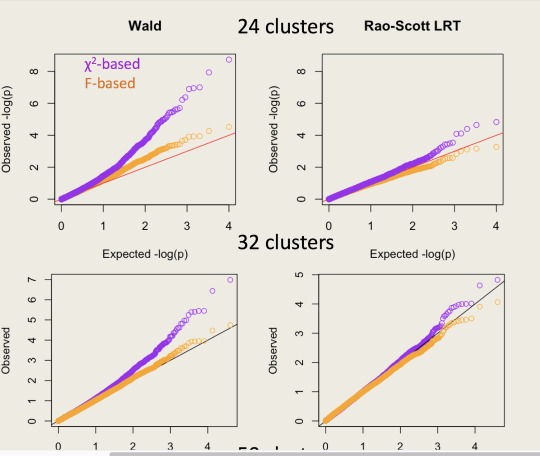
Here’s an example of qqplots of $-\log_{10} p$-values simulated  in a Cox model: the Wald test is the top panel and the Rao--Scott LRT is the bottom panel. The clusters are of size 100; the orange tests use the design degrees of freedom minus the number of parameters as the denominator degrees of freedom in an $F$ test. 

So, what’s new? SUDAAN has tests they call “Satterthwaite Adjusted Wald Tests”, which are based on $(\hat\beta-\beta_0)^T\hat V_0^{-1} (\hat\beta-\beta_0)$.  I’ve added similar tests to version 3.33 of the survey package (which I hope will be on CRAN soon).  These new tests are (I think) asymptotically locally equivalent to the Rao--Scott LRT and score tests. I’d expect them to be slightly inferior in operating characteristics just based on traditional folklore about score and likelihood ratio tests being better. But you can do the simulations yourself and find out. 

The implementation is in the regTermTest() function, and I’m calling these “working Wald tests” rather than “Satterthwaite adjusted”, because the important difference is the substitution of $V_0$ for $V$, and because I don’t even use the Satterthwaite approximation to the asymptotic distribution by default. 

[notstatschat]

As far as it goes

I’ve been reading two somewhat depressing documents today.

The American Statistical Association has put out a position paper titled “Overview of Statistics as a Scientific Discipline and Practical Implications for the Evaluation of Faculty Excellence“. It says, in the executive summary

Statistics is at the same time a dynamic, stand-alone science with its own core research agenda and an inherently collaborative discipline, developing in response to scientific needs. In this sense, statistics fundamentally differs from many other domain-specific disciplines in science. This difference poses unique challenges for defining the standards by which faculty excellence is evaluated across the teaching, research, and service components.

This document strives to provide a conceptual framework and practical guidelines to facilitate such evaluations. To that end, the intended audience includes all participants in the evaluation process—provosts and deans with faculty members in statistics positions; chairs and heads of statistics, biostatistics, and non-statistics departments; and the promotion and tenure evaluation committees in academic institutions.Furthermore, this document seeks to assist statistical scientists in the negotiation of faculty positions and the articulation of their collaborative role with the subject-matter sciences.

The position paper references a paper from a few years ago called “Evaluating Academic Scientists Collaborating in Team-Based Research: A Proposed Framework”. The latter is by people in biostatistics/epi (the former, rather notably, has no names from biostatistics departments).  They both deal with the question of how to get people promoted when they do a lot of collaborative research rather than sitting in an office proving theorems.

Both papers are good as far as they go. But, as Di Cook and others pointed out on Twitter, one of the places they don’t go is where most modern statistics lives. There is no mention of “computing”, “programming”, or “software”,  “open” or “reproducible”. Twenty years ago, this lack would have been unfortunate but unremarkable. Today, it’s bizarre. 

So, what should the position paper say about computing? Here’s a start:

Statistical software development and publishing is also “a legitimate and essential scholarly activity” for the discipline.

Data analysis is part of statistics, so that research on the theory, practice, and teaching of data analysis is statistics research

Software may be important either because it contributes to the discipline of statistical computing, or because it improves the quality of research in other areas of science (or both). 

Software often develops over time: peer review before initial publication may be neither necessary nor sufficient

Some statistical computing is crap; knowledgeable evaluation is necessary.

Recognising that expertise may be hard to find, the ASA (or other relevant bodies) should assist departments in finding reviewers to evaluate statistical computing and data science research

Department chairs should make sure expectations and criteria are clear.

[Two clarifications: 

for 6. A set of explicit criteria would be much better, but i think it’s easier to get agreement on particular cases than to get agreement on a set of criteria -- a workshop in 2001 didn’t manage.

for 7: what the expectations and criteria are, not what they should be-- if your department is not going to promote someone without an Annals paper, you need to know that]

[notstatschat]

breakInNamespace

Attention Conservation Notice: I’m putting this in a blog post in the hope it makes it easier for other people to find when they encounter the problem. 

The !! and !!! quasiquotation syntax in R’s tidyverse will break if you run them through the parser and deparser. This means:

Printing out the code of a function at the command line may give the wrong code

Functions like fix(), fixInNamespace(), and edit() may break functions using quasiquotation.

When you’re stepping through a function in the debugger, the code the debugger displays may be wrong

I say “may” because it depends on your settings for saving the source code of functions. By default, the problems occur with code loaded in packages but not for code loaded by source().

The symptom is that you get bizarre-looking nested calls to the ! operator. For example, from the tidypredict package

reg <- expr(!(!syms(reg)))

and

reduce(set, function(l, r) expr((!(!(!l))) * (!(!(!r)))))

The output from these functions ends up with lots of exclamation marks in it, and doesn’t work. 

Tracking this down is quite hard -- especially when you’ve been trained over the years that “it’s never the compiler”.  Sometimes it is (or, rather, the interpreter).

What’s happening under the hood? The tidyeval system has a special magic interpreter to treat !! and !!! as single operators. This is possible because R does, in fact, distinguish !!x from !(!x)) at the level of the parse tree. Things break because the deparser doesn’t distinguish.

Why does the deparser not distinguish? I don’t know for sure, but I suspect it’s because the operator precedence of ! is not what many people would expect: it binds relatively loosely, so that !x %in% y is the same as !(x %in% y). Putting in the implied parenthesis (previously) made code more readable, and it wouldn’t cause any problems under the built-in definition of ! as the logical not operator. With tidyeval, we have problems. 

Now,  I like quasiquotation. I’m responsible for the previous step in this direction, the bquote() function. I don’t want to get into the fight over whether !! is an abomination or a brilliantly creative work-around.

The fact that C++ overloads the bitwise left shift operator to do printing is probably a supporting argument that could be used in the fight -- but I’m not sure by which side.   

[notstatschat]

Finding packages

R, as I’ve pointed out before, has a package discovery problem.

There’s a new package, colorblindr, which lets you see the impact of various sorts of colour-blindness on a colour palette, a very useful thing for designing good graphics. When it’s mentioned on Twitter, you see lots of people glad that such a tool is now available for R. 

A similar tool has been available on CRAN for fifteen years. 

Now, the new package looks to have a better representation of colour vision. The dichromat package used colour-matching experiments from the 1990s and interpolates with loess; colorblindr seems to have a unified colour model.   It would be nice to see a comparison of the two packages, and maybe it would show everyone should move to the new one.  That’s what’s happened to a lot of my contributions to R. Progress is good.

But my point right now is there are a lot of people excited about colorblindr who didn’t know dichromat existed. Most of these are people who would have been interested in dichromat but didn’t know about it.  I haven’t exactly been quiet about the package --for example, it’s in the R courses that Ken Rice and I teach around the world, and I wrote about it for the ASA Computing and Graphics newletter.  It’s not hard to get me to talk about color spaces; some people would say it’s hard to get me to stop.

CRAN Task Views have helped a bit with the package discovery problem -- but dichromat is in the Graphics task view. It helps if a popular package suggests yours -- but dichromat is a dependency of a dependency of ggplot2. It helps if the package author is reasonably well known or the package was on CRAN early -- but again. It would help to give a clearer name, perhaps?

There must be lots of people out there who would be excited to find there was a package doing just what they needed. But there isn’t an easy way for them to notice. 

[notstatschat]

e-bike-onomics

If you own an e-bike, you get used to certain questions: how fast does it go, how often does it need to be charged, how much did it cost?

My e-bike was a bottom-end one two years ago -- I didn’t know if I’d end up using it, so I didn’t spend more than I had to. Since then, the quality has generally gone up, and so has the price. Andrew Chen, who just bought one, says that reliable entry-level bikes are \$2500-\$3000. That’s quite a bit of money, but so are other commuting methods.

In the mornings, I take a train to Newmarket then ride to the University. In the evenings I ride all the way home.  That costs me \$1.85 for a train fare. Going by bus all the way both ways costs $6.30, so I save \$4.45 by cycling.  Since I often stop to go shopping on the way home I’d sometimes need to pay an extra fare on the bus -- and before Auckland Transport started proper transfers, shopping would always be an extra fare.

Suppose we use \$4.45/day as the benchmark. At 5 days a week --  reasonable, because while I miss some weekdays, I do ride at weekends too -- that’s \$1157/year. Over three years that’s over  \$3400 -- enough for an e-bike plus maintenance -- and even the battery should last substantially longer than that.

You might think I need to add the cost of electricity: I pay about 30c per kWh; a complete charge is about 1/3 kWh; I probably average less than 3 charges per week. Over three years that’s maybe \$50. 

Now, I’ve got some important advantages here. I can often leave work earlier or later to avoid rain -- and if necessary leave my bike there overnight. Also, I’m at the very end of a train line, so I can be sure of getting my bike on the train in the morning. Still, it’s notable how quickly a bike pays off compared to bus fares -- and the comparison to University parking permit would be even more favourable. Obviously the numbers for a conventional bike would be dramatically better -- but since I’m not going to commute on a conventional bike, that’s not really relevant.  

When electric bikes are expensive but cost-saving at plausible discount rates, there’s interesting potential for employers to subsidise them. 

[notstatschat]

Statistics on pairs

I'm interested in estimation for complex samples from structured data --- clustered, longitudinal, family, network --- and so I'm interested in intuition for estimating statistics of pairs, triples, etc.   This turns out to be surprisingly hard, so I want easy examples.  One thing I want easy examples for is the relationship between design-weighted $U$-statistics and design-weighted versions of their Hoeffding projections. That is, if you write a statistic as a sum over all pairs of observations, you can usually rewrite it as a sum of a slightly more complicated statistic over single observations, and I want to think about whether the weighting should be done before or after you rewrite the statistic.

The easiest possible $U$-statistic is the variance $$V = \frac{1}{N(N-1)}\sum_{i,j=1}^N (X_i-X_j)^2$$ where Hoeffding projection gives the usual form $$S = \frac{1}{N-1} \sum_{i=1}^N (X_i-\frac{1}{N}\sum_{j=1}^N X_j)^2.$$

These are identical, as everyone who has heard of $U$-statistics has probably been forced to prove.  In fact $$\begin{eqnarray*} S&=& \frac{1}{N-1}\sum_{i=1}^N (X_i - \frac{1}{N}\sum_{j=1}^N X_j)^2\\\\ &=&\frac{1}{N-1}\sum_{i=1}^N \left(\frac{1}{N}\sum_{j=1}^N (X_i-X_j)\right)^2\\\\ &=&\frac{1}{N-1}\sum_{i=1}^N \left(\frac{1}{N}\sum_{j=1}^N (X_i-X_j)\right)^2\\\\ &=&\frac{1}{N(N-1)}\sum_{i,j=1}^N (X_i-X_j)^2 + \frac{1}{N(N-1)}\sum_{(i,j)\neq(k,l)}^N (X_i-X_j)(X_k-X_l)\\\\ \end{eqnarray*}$$ with the second term zero by symmetry, because the $(i,j)$ terms cancel the $(j,i)$ terms and so on.

The idea is that we can estimate $S$ from a sample by putting in sampling weights $w_i$ where $w_i^{-1}$ is the probability of $X_i$ getting sampled, because the sums are only over one index at a time.  We get a weighted mean with another weighted mean nested inside it.   We can reweight $V$ with pairwise sampling weights $w_{ij}$ where $w_{ij}^{-1}$ is the probability that the pair $(i,j)$ are both sampled, because the sum is over pairs.  

Under general sampling, we'd expect the two weighted estimators to be different because one of them depends on joint sampling probabilities and the other doesn't. Unfortunately, the variance is too simple. For straightforward comparisons such as simple random sampling versus cluster sampling all the interesting stuff cancels out and the two estimators are the same. We do not pass `Go' and do not collect 200 intuition points.

The next simplest example is the Wilcoxon--Mann--Whitney test.

Setup

Suppose we have a finite population of pairs $(Z, G)$ , where $Z$ is numeric and $G$ is binary, and for some crazy reason we want to do a rank test for association between $Z$ and $G$.  In fact, we don't {\bf need} to assume we want a rank test, since the test statistics will be reasonable estimators of well-defined population quantities, but to be honest the main motivation is rank tests.  For a test to make any sense at all, we need a model for the population, and we'll start with pairs $(Z,G)$ chosen iid from some probability distribution. Later, we'll add covariates to give a bit more structure.

Write $N$ for the number of observations with $Z=1$ and $M$ for the numher with $Z=0$, and write $X$ and $Y$ respectively for the subvectors of $Z$. Write $\mathbb{F}$ for the empirical cdf of $X$, $\mathbb{G}$ for the empirical cdf of $Y$, and $\mathbb{H}$ for that of $Z$.  

The Mann--Whitney $U$ statistic (suitably scaled) is $$U_{\textrm{pop}} = \frac{1}{NM} \sum_{i=1}^N\sum_{j=1}^M \{X_i>Y_j\}$$ The Wilcoxon rank-sum statistic (also scaled) is $$W_{\textrm{pop}} = \frac{1}{N}\sum_{i=1}^N \mathbb{H}(X_i) -\frac{1}{M}\sum_{J=1}^M \mathbb{H}(Y_j)$$

Clearly, $U_\textrm{pop}$ is an unbiased estimator of $P(X>Y)$ if a single observation is generated with $G=0$ and $G=1$.  We can expand $\mathbb{H}$ in terms of pairs of observations: $$\mathbb{H}(x) = \frac{1}{M+N}\left(\sum_{i=1}^N \{X_i\leq x\} + \sum_{j=1}^M \{Y_j\leq x\}\right)$$ and substitute to get $$\begin{eqnarray*} W_{\textrm{pop}} &= &\frac{1}{N}\sum_{i=1}^N \frac{1}{M+N}\left(\sum_{i'=1}^N \{X_{i'}\leq X_i\} + \sum_{j'=1}^M \{Y_{j'}\leq X_i\}\right) \\\\ & &\qquad - \frac{1}{M}\sum_{j=1}^M \frac{1}{M+N}\left(\sum_{i'=1}^N \{X_{i'}\leq Y_j\} + \sum_{j'=1}^M \{Y_{j'}\leq Y_j\}\right)\\\\ &=& \frac{1}{N(M+N)} \sum_{i=1}^N\sum_{j'=1}^M  \{Y_{j'}\leq X_i\}-\frac{1}{M(M+N)}  \sum_{i'=1}^N \{X_{i'}\leq Y_j\} \\\\ &&\qquad +\frac{1}{N(M+N)}\sum_{i=1}^N\sum_{i'=1}^N \{X_{i'}\leq X_i\} - \frac{1}{M(M+N)}\sum_{j=1}^M\sum_{j'=1}^M \{Y_{j'}\leq Y_j\}\\\\ &=&\frac{M+N}{NM(M+N)}\sum_{i,j} \{X_i>Y_j\} + \frac{NM(M-1)/2-MN(N-1)/2}{NM(M+N)}\\\\ &=&\frac{1}{NM}\sum_{i,j} \{X_i>Y_j\} + \frac{M-N}{2(M+N)} \end{eqnarray*}$$

So,  $$U_\textrm{pop} =  W_\textrm{pop} + \frac{M-N}{2(M+N)}$$ and the two tests are equivalent, as everyone already knows. Again, there's a good chance you have been forced to do this derivation, and you probably took fewer tries to get it right than I did.

Definitions under complex sampling

We take a sample, with known marginal sampling probabilities $p_i$ for the $X$s, $q_j$ for the $Y$s and pairwise sampling probabilities $\pi_{i,j}$.  We write $n$ and $m$ for the number of sampled observations in each group, and relabel so that these are $i=1,\ldots,n$ and $j=1,\ldots,m$.  We write $\hat N$  and $\hat M$ for the Horvitz--Thompson estimates of $N$ and $M$, and $\hat F$ for the estimate of $\mathbb{F}$ (and so on).  That is $$\hat H(z) = \frac{1}{\hat M+\hat N}\left(\sum_{i=1}^n \frac{1}{p_i} \{X_i\leq z\} + \sum_{j=1}^m \frac{1}{q_i} \{Y_j\leq z\}\right)$$

The natural estimator of $W_\textrm{pop}$ is that of Lumley and Scott $$\hat W = \frac{1}{\hat N}\sum_{i=1}^n \frac{1}{p_i}\hat{H}(X_i) -\frac{1}{\hat M}\sum_{J=1}^m \frac{1}{q_i}\hat{H}(Y_j)$$

A natural estimator of $U_\textrm{pop}$ is $$\hat U= \frac{1}{\widehat{NM}} \sum_{i=1}^n\sum_{j=1}^m \frac{1}{\pi_{ij}}\{X_i>Y_j\}$$

Now

 $\hat U$ and $\hat W$ are consistent estimators of the population values

 Therefore, they are also consistent estimators of the superpopulation parameters

However, $\hat U$ depends explicitly on pairwise sampling probabilities and $\hat W$ does not

And there (hopefully) isn't enough linearity to make all the differences go away.

Expansions

We can try to substitute the definition of $\hat H$ into the definition of $\hat W$ and expand as in the population case.  To simplify notation I will assume that the sampling probabilities are designed or calibrated so that $N=\hat N$ and so on (or close enough that it doesn't matter). $$\begin{eqnarray*} \hat W &= &\frac{1}{N}\sum_{i=1}^n \frac{1}{p_i} \frac{1}{M+N}\left(\sum_{i'=1}^n \frac{1}{p_{i'}}\{X_{i'}\leq X_i\} + \sum_{j'=1}^m \frac{1}{q_{j'}} \{Y_{j'}\leq X_i\}\right) \\\\ & &\qquad - \frac{1}{M}\sum_{j=1}^m \frac{1}{q_{j}} \frac{1}{M+N}\left(\sum_{i'=1}^n\frac{1}{p_{i'}} \{X_{i'}\leq Y_j\} + \sum_{j'=1}^m\frac{1}{q_{j'}} \{Y_{j'}\leq Y_j\}\right)\\\\ &=& \frac{1}{N(M+N)} \sum_{i=1}^n\sum_{j'=1}^m\frac{1}{p_iq_{j'}}  \{Y_{j'}\leq X_i\}-\frac{1}{M(M+N)}  \sum_{i'=1}^n \sum_{j=1}^m\frac{1}{p_{i'}q_{j}} \{X_{i'}\leq Y_j\} \\\\ &&\qquad +\frac{1}{N(M+N)}\sum_{i=1}^n\sum_{i'=1}^n \frac{1}{p_{i'}p_{i}} \{X_{i'}\leq X_i\} - \frac{1}{M(M+N)}\sum_{j=1}^m\sum_{j'=1}^m \frac{1}{q_jq_{j'}} \{Y_{j'}\leq Y_j\}\\\\ &=&\frac{1}{MN}\sum_{i,j}\frac{1}{p_iq_j} \{X_i>Y_j\} + \textrm{ugly expression not involving $X$ and $Y$} \end{eqnarray*}$$

(The ugly expression involves the variance of the marginal sampling weights, since $$2\sum_{i,i'} p_i^{-1}p_{i'}^{-1}= (\sum_i p_i^{-1})^2- 2\sum_i p_i^{-2}.$$ It doesn't depend on $X$ and $Y$, and it is the same in, for example, simple random sampling of individuals and simple random sampling of clusters. )

That is, the reweighted $\hat W$ is a version of $\hat U$ using the product of marginal sampling probabilities rather than the joint ones.  They really are different, this time. Using $\hat W$ will give more weight to pairs within the same cluster than to pairs in different clusters.

It’s still not clear which one is preferable, eg,  how will the power of the tests compare in various scenarios? But it’s progress. 

[notstatschat]

How to add chi-squareds

A quadratic form in Gaussian variables has the same distribution as a linear combination of independent $\chi^2_1$ variables -- that’s obvious if the Gaussian variables are independent and the quadratic form is diagonal, and you can make that true by change of basis. The coefficients in the linear combination are the eigenvalues $\lambda_1,\dots,\lambda_m$ of $VA$, where $A$ is the matrix representing the quadratic form and $V$ is the covariance matrix of the Gaussians. I’ve written about the issue of computing the eigenvalues, and how to speed this up. That still leaves you with the problem of computing tail probabilities for a linear combination of $\chi^2$s -- for $m$ at least hundreds, and perhaps thousands or tens of thousands. 

There’s quite a bit of literature on this problem, but it mostly deals with small numbers of terms (like, say, $m=5$) and moderate p-values.  The genetics examples involve large numbers of terms and very small p-values. So, Tong Chen did an MSc short research project with me, looking at these methods in the context of genetics. Here’s a summary of what we know (what we knew before and what he found)

‘Exact’ methods

Farebrother: based on an infinite series of $F$ densities

Davies: based on numerical inversion of the characteristic function

Bausch: based on an algebra for sums of Gamma distributions

All three of these can achieve any desired accuracy when used with infinite-precision arithmetic. Bausch’s method also has bounds on the computational effort, polynomial in the number of terms and the log of the maximum relative approximation error.

In ordinary double-precision (using Kahan summation), Bausch’s method can be accurate in the right tail for 50 or so terms. It is very inaccurate in the left tail. Achieving anything like the full theoretical accuracy of the algorithm requires multiple-precision arithmetic and seems slow compared to the alternatives. (It might be faster in Mathematica, which is what Bausch used)

Farebrother’s method and Davies’s method are usable even for a thousand terms, and achieve close to their nominal accuracy as long as the right tail probability is much larger than machine epsilon.  Since $P(Q>q)$ is computed from $1-P(Q<q)$, they break down completely at right tail probabilities near machine epsilon. Farebrother’s method is faster for high precision, but only works when all the coefficients are positive. 

Moment methods

The traditional approach is the Satterthwaite approximation, which approximates the distribution by $a\chi^2_d$ with $a$ and $d$ chosen to give the correct mean and variance.  The Satterthwaite approximation is much better than you’d expect for moderate $p$-values and is computationally inexpensive: it only needs the sum and sum of squares of the eigenvalues, which can be computed more rapidly than the full eigendecomposition and can be approximated by randomised estimators.

Sadly, the Satterthwaite distribution is increasingly anti-conservative in the right tail.

Liu and co-workers proposed a four-moment approximation by a distribution of the form $a+b\chi^2_d(\nu)$, where $\nu$ is a non-centrality parameter and $a$ is an offset. This approximation is used in the R SKAT package. It’s a lot better than the Satterthwaite approximation, but it is still anticonservative in the right tail, even for $p$-values in the vicinity of $10^{-5}$.

The moment methods are more-or-less inevitably anticonservative in the right tail, because the extreme right tail of the linear combination is proportional to the extreme right tail of the single summand $\lambda_1\chi^2_1$ corresponding to the leading eigenvalue. (That’s how convolutions with exponential tails work.) The tail of the approximation depends on all of the eigenvalues and so is lighter. 

Moment methods more accurate than the Satterthwaite approximation need summaries of the third or higher powers of the eigenvalues; these can’t be computed any faster than by a full eigendecomposition.

Saddlepoint approximation

Kuonen derived a saddlepoint approximation to the sum. The approximation gets better as $m$ increases. Tong Chen proved it has the correct exponential rate in the extreme right tail, so that its relative error is uniformly bounded. The computational effort is linear in $m$ and is fairly small. On the downside, there’s no straightforward way to use more computation to reduce the error further.

Leading eigenvalue approximation

This approximates $\sum_{i=1}^m\lambda_i\chi^2_1$ by a sum of $k$ terms plus a remainder $$a_k\chi^2_{d_k}+\sum_{i=1}^k\lambda_i\chi^2_1$$

The remainder is the Satterthwaite approximation to the $n-k$ remaining terms; having the first $k$ terms separate is done to improve the tail approximation.  You still need to decide how to add up these $k+1$ terms, but the issues are basically the same as with any set of $k+1$ $\chi^2$s.

Take-home message

For large $m$, use the leading-eigenvalue approximation

For p-values much larger than machine epsilon, use the Davies or Farebrother algorithms (together with the leading-eigenvalue approximation if $m$ is large)

For p-values that might not be much larger than machine epsilon, use the saddlepoint approximation if its relative error (sometimes as much as 10% or so) is acceptable. There’s no need to use the leading-eigenvalue approximation if you have the full set of eigenvalues, but you might want to use it to avoid needing them all. 

If you need very high accuracy for very small tail probabilities, you’ll need Bausch’s method, and multiple-precision arithmetic. With any luck you’ll still be able to use the leading-eigenvalue approximation to cut down the work. 

[notstatschat]

Secret Santa collisions

Attention Conservation Notice: while this probability question actually came up in in real life, that’s just because I’m a nerd.

“Secret Santa” is a Christmas tradition for taming the gift-giving problem in offices, groups of acquaintances, etc. Instead of everyone wondering which subset of people they should give a gift to, each person is randomly assigned one recipient and has to give a gift (with a relatively low upper bound on cost) to that one person. The ‘Secret’ part is that you don’t know who is going to give you the gift. 

It’s not completely trivial (though it’s not that hard) to come up with a random process that assigns everyone exactly one recipient and ensures that no-one is left finding a gift for themselves.  One procedure is to sample recipients without replacement to get a list that’s guaranteed to be one-to-one, and then just repeat the sampling until you get an allocation where no-one is assigned themselves. 

So, a probability question: how likely is it that a random permutation will have ‘collisions’ where someone is their own Secret Santa? Or, equivalently, how many tries would you expect to need to get a working allocation? Does it depend on the number of people $n$? What about for 3600 people, as in the scheme hosted by NZ Post on Twitter.  

I knew the answer, but I didn’t know a proof, so this is a reasonably honest exploration of how you might find the answer.

First, is there some simple bound? Well, the chance that you, Dear Reader, get assigned yourself is $1/n$, so the simple Bonferroni bound is $n\times 1/n$. That doesn’t look very helpful, because we already knew 1 was an upper bound; this is a probability.  However, we  can recast the Bonferroni bound as the expected number of collisions.  If the expected number of collisions is 1, then it’s reasonable to expect that the probability of no collisions is appreciable, and that as $n$ increases it converges to some useful number that isn’t 1 or 0.  At this point, if you had to make a wild guess, a reasonable guess would be that the number of collisions has approximately a Poisson distribution for large $n$, so that the probability of no collisions will be approximately $e^{-1}$.

Next, try simulation. Doing $10^5$ replicates in R gives

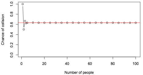
The probability is 1 if you try to do this by yourself, 1/2 if you have one friend, and converges astonishingly quickly to a fixed value.  The red line is $1-e^{-1}$.

Now, can we prove this? The collisions aren’t independent, so we can’t quite just use a Poisson or Binomial argument. We could try the higher-order Bonferroni bounds, eg $$P(\cup_i A_i)\geq \sum_i P(A_i) - \sum_{i,j} P(A_i\cap A_j).$$

The second-order bound gives $n\times 1/n-{n\choose 2}\times 1/n^2=1/2$, so we’re making progress.  The third-order bound gives $$n\times 1/n-{n\choose 2}\times 1/n^2+{n\choose 3}\times 1/n^3=1-1/2+1/6=4/6$$

We’re definitely making progress now, and these bounds look suspiciously like the values of the probability for $n=1,\,2,\,3$.  Continuing the pattern, we will end up with $$\sum_{k=1}^\infty (-1)^{k+1}{n\choose k} n^{-k}=\sum_{k=1}^\infty \frac{(-1)^{k+1}}{n^{-k}}$$

Comparing that to the infinite series for $\exp(x)$, it’s $1-e^{-1}$. What we haven’t got this way is whether the number of collisions is Poisson, which was where the guess originally came from. This seems to be a lot harder.  

First, simulation confirms that the Poisson is a good approximation. That’s reassuring: it’s typically easier to prove things that are true than things that are not true. 

I should next say that I spent quite a long time looking for ‘coupling’ arguments to show that this assignment method gave the same large-sample distribution as some other assignment method that was obviously Poisson. I didn’t get anywhere with this, but it’s a fruitful approach for problems similar to this one. Since that didn’t work, we’re back to combinatorics.

Now, suppose we have 1 collision. That means we have an assignment of the $n-1$ other people with no collisions. So, the number of ways to have 1 collision in $n$ people is $n$ times the number of ways to have no collisions in $n-1$ people. Since the number of permutations of $n$ people is also $n$ times the number of permutations of $n-1$ people, the fraction of permutations with 1 collision in $n$ people is the same as the fraction of permutations with 0 collisions in $n-1$ people, ie, for large $n$ it’s $e^{-1}$. That agrees with the Poisson formula, so we’re definitely making progress.

If we have $k$ collisions in $n$ people then we have a set of $n-k$ people with no collisions. The number of ways we can have $n-k$ people with no collisions is about $(n-k)!e^{-1}$ and the number of ways to pick the $k$ people who have to buy themselves gifts is ${n\choose k}= n!/(k!(n-k)!)$. So, the number of ways of having $k$ collisions in $n$ is about $n!e^{-1}/k!$, and the probability of this is $e^{-1}/k!$, matching the Poisson distribution. We’ve done it!

Ok. Technically we’re not quite done, since we’d need to show the approximation error in the argument actually gets smaller with increasing $n$. But we’re done enough for me. 

PS: If you want an easy way not to have to worry about collisions, just arrange the people in random order and assign each person the following person in the list (with the last person being assigned the first).