onblogg

[onblogg]

On Linear and Angular Momentum

In introducing Newton’s Laws, I introduced the linear momentum of a particle, defined as \[ \boldsymbol{p} = m \boldsymbol{v} \]We foreshadowed the importance of this quantity when we introduced Newton’s First Law, which stated that if there is no net force on a particle, its momentum is constant in time. That is, the momentum of the particle is conserved if no net force acts on it. By itself, it seems like Newton’s First Law isn’t very general. As we saw in the last essay, there exist some forces (like gravity) that act between any masses, so the chances of an individual particle having no net force acting on it seems incredibly slim. So why do we care about momentum, besides for defining Newton’s Laws? The astounding fact that makes momentum a quantity worth studying is that momentum conservation, what Newton’s First Law only states for individual particles, holds in general for collections of particles.

Suppose we have a collection of \(N\) particles and that those particles interact with some force. It doesn’t matter what form this force takes, all that matters is that there exists some force between them. In general, there may also be an external force acting on the system as well. An example system might look like this

We can write down the force between each particle. The force on particle \(i\) due to particle \(j\) is written as \[ \boldsymbol{F}_{ij} \]

So we may ask, what is the total force acting on particle \(i\)? It’s the sum of all of the forces due to all other particles and the sum of the external force on particle \(i\). The net force is therefore \[ \boldsymbol{F}_{i}^{net} = \boldsymbol{F}_{i}^{ext} + \boldsymbol{F}_{i 1} + \boldsymbol{F}_{i 2} + … + \boldsymbol{F}_{i N} \]

Large sums like this show up a lot in math and physics. To simplify our equations, we use the summation notation. The above equation is equivalent to \[ \boldsymbol{F}_{net} = \boldsymbol{F}_{i}^{ext} + \sum_{i \neq j}^{N} \boldsymbol{F}_{ij} \]

Notice that in the sum I specified \(i \neq j\). Why did I do that? Well, what would the term \(\boldsymbol{F}_{ii}\) mean? This is the force on particle \(i\) due to particle \(i\). In other words, it’s the force of a particle on itself. However, a particle cannot exert a force on itself, so this is the statement that there is no self-force. We can write the net force in terms of the momentum, since Newton’s Second Law is \[ \boldsymbol{F}_{i}^{net} = \dot{ \boldsymbol{p} }_{i} \]

Therefore, we can plug in for the net force on particle \(i\) \[ \dot{ \boldsymbol{p} }_{i} = \boldsymbol{F}_{i}^{ext} + \sum_{i \neq j}^{N} \boldsymbol{F}_{ij} \]

The total momentum of this system is the sum of all individual momenta \[ \boldsymbol{P} = \sum_{i} \boldsymbol{p}_{i} \]

We can take a time derivative of this \[ \dot{\boldsymbol{P}} = \sum_{i} \dot{\boldsymbol{p}}_{i} \]

And plug in from Newton’s Second Law \[ \dot{\boldsymbol{P}} = \sum_{i} \left[\boldsymbol{F}_{i}^{ext} + \sum_{i \neq j}^{N} \boldsymbol{F}_{ij} \right] \]

\[ \dot{ \boldsymbol{P} } = \sum_{i} \boldsymbol{F}_{i}^{ext} + \sum_{i} \sum_{i \neq j}^{N} \boldsymbol{F}_{ij} \]

The first term, \(\sum_{i} \boldsymbol{F}_{i}^{ext}\), is just the sum of all external forces on all particles, so it is the total external force. We let \[ \boldsymbol{F}^{ext}_{tot} = \sum_{i} \boldsymbol{F}_{i}^{ext} \]

Then, we write \[ \dot{ \boldsymbol{P} } =\boldsymbol{F}_{tot}^{ext} + \sum_{i} \sum_{i \neq j}^{N} \boldsymbol{F}_{ij} \]

Here’s another thing that’s common in math and physics. Sometimes, we compactify too much information into the notation, so we lose track of what’s really important. There are times where it is important to unpack the notation to see what’s really going on. Let’s expand out this sum. It is \[ \dot{\boldsymbol{P}} = \boldsymbol{F}_{tot}^{ext} + \boldsymbol{F}_{12} + \boldsymbol{F}_{13} + ... + \boldsymbol{F}_{1N} + \boldsymbol{F}_{21} + \boldsymbol{F}_{23} + … + \boldsymbol{F}_{N (N-1)} \]

Why is expanding out this sum like this worth the effort? Well, we are free to group terms as we like. In particular, we can write this sum as \[ \left(\boldsymbol{F}_{12} + \boldsymbol{F}_{21} \right) + \left(\boldsymbol{F}_{13} + \boldsymbol{F}_{31} \right) + … \left(\boldsymbol{F}_{N (N-1)} + \boldsymbol{F}_{(N-1) N} \right) \]

See where we’re going yet? By grouping terms like this, we can make use of one of our fundamental laws. Specifically, Newton’s Third Law states \[ \boldsymbol{F}_{12} = - \boldsymbol{F}_{21} \]

Every action has an opposite and equal reaction, as they say. So we can use Newton’s Third Law in this sum to write \[ \left(\boldsymbol{F}_{12} - \boldsymbol{F}_{12} \right) + \left(\boldsymbol{F}_{13} - \boldsymbol{F}_{13} \right) + … \left(\boldsymbol{F}_{N (N-1)} - \boldsymbol{F}_{N(N-1)} \right) = 0 \]

So everything in that large, nasty sum cancels each other out. Each individual internal force has an equal and opposite corresponding force that exactly cancels it out. Returning to our full expression, we come to the vital result that  \[ \dot{\boldsymbol{P}} = \boldsymbol{F}_{tot}^{ext} \]

That is, the rate of change of the total momentum of the system only relies on the external forces! So what? What’s the utility of this fact? This will take a little more math to prove. We define the center of mass position, denoted by \(\boldsymbol{R}\) and given by \[ \boldsymbol{R} = \frac{ \sum_{i} m_i \boldsymbol{r}_i }{ \sum_{i} m_i } \]

The center of mass is the “mass-weighted sum” of position. The top of the fraction is just the sum of each individual particle position multiplied by its mass, and the bottom of the fraction is the total mass. We can denote the total mass as \[M = \sum_{i} m_i \]

Then, the equation for the center of mass is just \[ \boldsymbol{R} = \frac{1}{ M } \sum_{i} m_i \boldsymbol{r}_i  \]

Assume (as we usually do in classical mechanics) that the masses of the individual particles don't change. Recall that the total momentum of a collection of particles is simply the sum of all individual momenta \[ \boldsymbol{P} = \sum_{i} \boldsymbol{p}_{i} \]

Using \( \boldsymbol{p}_i = m_i \dot{\boldsymbol{r} }_i \), we can write \[ \boldsymbol{P} = \sum_{i} m_i \dot{\boldsymbol{r}}_i \]

Now, let’s take a time derivative of the center of mass position. \[ \dot{ \boldsymbol{R} }= \frac{1}{ M } \sum_{i}  m_i \dot{\boldsymbol{r}_i } \]

Multiplying by the total mass, we find \[ M \dot{ \boldsymbol{R} }= \sum_{i}  m_i \dot{\boldsymbol{r}_i } \]

Or, using our definition of the total momentum,

\[ \boldsymbol{P} =M \dot{ \boldsymbol{R} } \]

This is amazing! A collection of particles follows the exact same formula for its total momentum as a single point particle with mass \(M\) at the center of mass! In fact, the dynamics of a collection of particles is exactly the same as the dynamics of a point particle. To see this, we can take another time derivative to find

\[\dot{ \boldsymbol{P} } = M \ddot{ \boldsymbol{R} } \]

But from above, we saw that

\[ \dot{\boldsymbol{P}} = \boldsymbol{F}_{tot}^{ext} \]

So

\[\boldsymbol{F}_{tot}^{ext}= M \ddot{ \boldsymbol{R} } \]

In other words, the center of mass for a collection of particles follows Newton’s Second Law as if it were a single particle of mass \(M\).

We now know how to characterize the linear motion of a collection of particles using the center of mass and the total momentum. The particles are otherwise free to move around the center of mass, though. Those motions, rotations around a point, can be characterized through angular momentum.

Consider an arbitrary collection of particles. We define a center point, \(\mathcal{O}\), from which the distance to all of the particles are measured

Each particle has its own position vector, \( \boldsymbol{r}_i \), and its own momentum, \( \boldsymbol{p}_i\). We define the angular momentum as the cross product between position and momentum \[ \boldsymbol{\ell} = \boldsymbol{r} \times \boldsymbol{p} \]

Notice that from this definition, we can derive an analogous equation of motion to Newton’s Second Law \[ \frac{d \boldsymbol{\ell}}{dt}\]

\[ \frac{d}{dt} \left( \boldsymbol{r} \times \boldsymbol{p} \right) = \frac{d \boldsymbol{r} }{dt} \times \boldsymbol{p} + \boldsymbol{r} \times \frac{d \boldsymbol{p} }{dt} \]

\[ \boldsymbol{v} \times \boldsymbol{p} + \boldsymbol{r} \times \boldsymbol{F} \]

\[ m\left(\boldsymbol{v} \times \boldsymbol{v}\right) + \boldsymbol{r} \times \boldsymbol{F} \]

From the definition of the cross product, it is easy to see that the cross product of a vector with itself is zero, so that we are left with  \[ \dot{\boldsymbol{\ell}} =  \boldsymbol{r} \times \boldsymbol{F} \]

We define the vector \( \boldsymbol{\Gamma} =  \boldsymbol{r} \times \boldsymbol{F} \) as the torque on the particle such that the equation of motion is \[ \dot{\boldsymbol{\ell}} = \boldsymbol{\Gamma}\]

This is analogous to Newton’s Second Law \[ \dot{\boldsymbol{p}} = \boldsymbol{F} \]

Notice that both the angular momentum and the torque on a particle depend on where we define the center point to be. If the center point changes, the angular momentum and the torque also change.

Now, let’s apply these results to our collection of particles above. If we take the center point to be the center of mass, and we use the definitions of torque and angular momentum, a similar derivation to the one I did above will lead us to  \[ \dot{\boldsymbol{L}} = \boldsymbol{\Gamma}^{ext}_{tot} + \left(\boldsymbol{r}_1 - \boldsymbol{r}_2 \right) \times \boldsymbol{F}_{12} + \left(\boldsymbol{r}_1 - \boldsymbol{r}_3 \right) \times \boldsymbol{F}_{13} + … \]

Where \(\boldsymbol{L}\) is the total angular momentum of the system and \(\boldsymbol{\Gamma}^{ext}_{tot} \) is the net external torque on the system. The big difference between this derivation and the one above is that the terms \(\left(\boldsymbol{r}_i - \boldsymbol{r}_j \right) \times \boldsymbol{F}_{ij} \) don’t necessarily vanish. To make them vanish, we need to add in one more assumption. Using some vector math, we can see that the vector \(\left(\boldsymbol{r}_i - \boldsymbol{r}_j \right)\) points from particle \(j\) to particle \(i\). The magnitude of the cross product is given by \[ \left|\left(\boldsymbol{r}_{i}-\boldsymbol{r}_{j}\right)\times\boldsymbol{F}_{ij}\right|=\left|\boldsymbol{r}_{i}-\boldsymbol{r}_{j}\right|F_{ij}\sin\theta \]

If the angle between the force \(\boldsymbol{F}_{ij} \) and the vector \(\left(\boldsymbol{r}_i - \boldsymbol{r}_j \right)\) is zero, then the corresponding internal torque will vanish. This kind of force, a force that only points directly along the straight line between particles, is a kind of force that is so common that it gets its own name. It is a central force. Central forces show up in lots of places in physics, but by far the most common examples are the gravitational force and the electric force. If we assume that all forces between the particles are central forces, then we are left with \[ \dot{\boldsymbol{L}} = \boldsymbol{\Gamma}^{ext}_{tot} \]

In other words, for a closed system of particles where the particles interact through central forces, both the internal forces and the internal torques cancel so that the entire motion of the system is governed only by the external forces and torques.

Normally, a course on mechanics would stop here to discuss by far the most important and practical reasons for introducing linear and angular momentum: conservation laws. I will briefly mention that if there are no external forces or torques on a system, then we have the equations \[ \dot{\boldsymbol{P}} = 0 \]

\[ \dot{\boldsymbol{L}} = 0 \]

Consequently, \[ \boldsymbol{P} = \text{constant} \]

\[ \boldsymbol{L} = \text{constant} \]

So, in the absence of external forces and torques, linear and angular momentum are constant throughout the entire motion of the system. When such a value stays constant over time, we say that the quantity is conserved. I am going to leave further discussion of conservation laws for after we have discussed the Lagrangian formulation. Right now, it appears that momentum conservation is a neat coincidence that occurs when a system is set up just right. After we have discussed the Lagrangian formulation, we will see that the conservation laws are the consequence of the symmetries of nature.

So for now, I want to start building towards the Lagrangian. This will take some more math and an introduction to the concept of energy. I will start developing that math in the next essay.

[onblogg]

On Basic Force Laws

Let’s consider three basic force laws that generate some surprising dynamics. As we will come to see, physics is very intimately tied to the study of differential equations. Newton’s Second Law is a differential equation, and the solutions that come from it will vastly change depending on the force law we’re studying.

Let’s begin with the simplest force possible, a constant force. This force will be constant in magnitude and direction for all times. We can arbitrarily define the direction of the force as the \(\hat{x}\) direction, so the force law is written as \[ \boldsymbol{F} = F_0 \hat{x}\]

We can then plug this into Newton’s Second Law to get \[ F_0 \hat{x} = m \ddot{ \boldsymbol{x} } \]

Writing \( \boldsymbol{x} \) in terms of its components, \( \boldsymbol{x} = x \hat{x} + y \hat{y} + z \hat{z} \), gives \[ F_0 \hat{x} = m \ddot{ x \hat{x}} + m \ddot{y \hat{y}} + m \ddot{z \hat{z}} \]

For two vectors to be equal, their components must be individually equal. So we have three equations \[ F_0 = m \ddot{x} \]

\[ 0 = m \ddot{y} \]

\[ 0 = m \ddot{z} \]

Dividing each equation by \(m\) gives \[ \frac{F_0}{m} =  \ddot{x} \]

\[ 0 =  \ddot{y} \]

\[ 0 =  \ddot{z} \]

These are three kinematic equations for each component of \(\boldsymbol{x}\). The equations for \(y\) and \(z\) imply constant velocity in those directions. Notice how when a force acts along one direction, the corresponding acceleration occurs in only that direction. In other words, the three directions are independent of each other.

Well, that wasn’t so exciting, but it should be reassuring that a constant force leads to a constant acceleration. What’s just a little more complicated than a constant force? A linear force! Specifically, let’s consider Hooke’s Law. Again, it describes a force that acts in one direction. Since we saw above that the other directions are independent, let’s just consider the one-dimensional motion resulting from this force law. Hooke’s Law states \[ F = -k x \]

Robert Hooke originally proposed this law as a model for springs. The distance \(x\) is measured as the displacement from the spring’s equilibrium position. As you stretch or compress the spring, the resulting force always tries to bring you back towards that equilibrium position and gets stronger the further away you get from equilibrium. Obviously, this is a brutalized model for a spring since real springs will overstretch and break if you stretch them enough. Nevertheless, this problem, the harmonic oscillator, is one of the most important problems in physics, though it will take some time before we can fully appreciate it. Once we introduce energy and approximation, I will dedicate an entire essay to the harmonic oscillator.

For now, let’s solve Newton’s Law for the harmonic oscillator. Plugging in Hooke’s Law gives us \[ -k x = m \ddot{x} \]

Moving all of the terms over to one side, we get \[ m \ddot{x} + k x = 0 \]

Dividing through by \(m\), we obtain \[ \ddot{x} + \frac{k}{m} x = 0 \]

For convenience, I will define a new symbol for the collection of constants. We will see the importance and significance of the name later, but for now I define \( \omega_{0}^{2} = \frac{k}{m} \) so that the equation becomes \[ \ddot{x} + \omega_{0}^{2} x = 0 \]

Now, we have to learn how to solve differential equations. Usually, the first step in solving any differential equation is to guess at a solution. For instance, if we guess that \( x\left(t\right) = t \), we can plug this guess into the equation and see if it gives us a true statement. Obviously, this guess doesn’t work. We can try many other, more sophisticated guesses, but fortunately many generations of mathematicians and physicists have made many guesses for us which we can look up. I will discuss more general methods of approaching differential equations like this in the future, but for now I will just quote the answer. There are two solutions to this differential equation, \[ x_{1} \left(t\right) = \sin\left( \omega_{0} t\right) \]

\[ x_{2} \left(t\right) = \cos\left( \omega_{0} t\right) \]

If you are unconvinced that these are solutions, just plug them in and you will see that they work out. In fact, those functions alone aren’t the only ones that work. Since our differential equation is linear, any linear combination of these two solutions is also a solution. That is, the most general solution is \[ x \left(t\right) = A \cos\left( \omega_{0} t\right) + B \sin\left( \omega_{0} t\right) \]

Let’s discuss the importance of each part of the solutions. First, the role of  \( \omega_0 \) becomes clear. If we have any sinusoidal function in time, the number multiplying the time is the frequency of the oscillation. In this case, \( \omega_0 \) is the natural frequency of the oscillator. Next, the two solutions, \( \cos\left( \omega_{0} t\right) \) and \( \sin\left( \omega_{0} t\right) \), represent slightly different motions. Both are oscillations with frequency \(\omega_0\), but each solution specifies a different position at \(t = 0\). The cosine solution corresponds to the spring being fully extended at \(t = 0\), while the sine solution corresponds to the spring being in equilibrium \(t = 0\). Finally, the two arbitrary constants \(A\) and \(B\) represent the amplitudes of the oscillation. Since sine and cosine are bounded between \(-1\) and \(1\), if you multiply those functions by any constant \(C\), the resulting function will be bounded between \(-C\) and \(C\).

The solution we obtained above is a general solution. To obtain a particular solution, we need two initial conditions to specify both constants. Typically, these conditions are given as the initial position and velocity of the particle. For instance, if we specify that \( x\left(0\right) = L \) and \( \dot{x} \left(0\right) = 0 \), we could plug into the general solution and solve \[ x\left(0\right) = A \cos\left( 0 \right) + B \sin\left( 0 \right) \]

\[ x\left(0\right) = A \]

\[ A = L \]

To solve for the second initial condition, we take one derivative \[ \dot{x}\left(t\right) = -A\omega_0 \sin\left(\omega_{0} t\right) + B \omega_0 \cos\left(\omega_{0} t\right) \]

Then we plug in for the initial condition \[ \dot{x}\left(0\right) = -A\omega_0 \sin\left(0\right) + B \omega_0 \cos\left(0\right) \]

\[ \dot{x}\left(0\right) = B \omega_0 \]

\[ B \omega_0 = 0 \]

\[B = 0 \]

This would give us the particular solution \[ x\left(t\right) = L \cos\left( \omega_{0} t\right) \]

We could introduce many more complications into the harmonic oscillator, but I’m going to postpone discussion of these complications until later. For now, we’ll just leave this as one simple example of a force law. A more complicated force law (in fact, perhaps the most complicated that Newton himself presented in the Principia), is Newton’s Law of Universal Gravitation. This law simply states that all masses in the universe have an attractive force between them. This attractive force is proportional to the product of the two object’s masses and inversely proportional to the square of their distances. In vector form, this law states \[ \boldsymbol{F} = -G \frac{m_1 m_2}{ \left| \boldsymbol{r}_1 - \boldsymbol{r}_2 \right|^2 } \hat{r} \]

Here, \(m_1\) and \(m_2\) are the masses of particles 1 and 2, \( \boldsymbol{r}_1 \) and \( \boldsymbol{r}_2  \) are the position vectors of particles 1 and 2, \(\hat{r}\) is the direction pointing from one particle to the other, \(G\) is the Universal Gravitation constant, and the minus sign is there to signify that the force is always attractive.

I’m not going to solve Newton’s Second Law for this force. That’s just asking for a world of pain at this point! We would need to write Newton’s Law in polar coordinates, then solve a pretty nasty looking differential equation. I’m going to save discussion of the trajectories that this law produces for when we have thoroughly discussed energy and both forms of momentum. For now, I just want to make some basic observations about this law and make some historical remarks.

Let’s begin by examining what happens when we plug in this law into Newton’s Second Law. We are examining the force on particle 1, so Newton’s Second Law reads \[  -G \frac{m_1 m_2}{ \left| \boldsymbol{r}_1 - \boldsymbol{r}_2 \right|^2 } \hat{r} = m_1 \ddot{\boldsymbol{x}} \]

\[  -G \frac{ m_2}{ \left| \boldsymbol{r}_1 - \boldsymbol{r}_2 \right|^2 } \hat{r} = \ddot{\boldsymbol{x}} \]

An interesting thing happens here. The mass \(m_1\) drops out of the equation! The same thing happens when we consider the force on \(m_2\). This means that if we are the force acting on, let’s say, the Earth by the Sun only depends on the Sun’s mass!

We can freely place one of the particles at the origin of our coordinate system. Let’s place particle 2 at the origin. Newton’s Second Law then reads \[  -G \frac{m_2}{ \left| \boldsymbol{r}_1 \right|^2 } \hat{r} = \ddot{\boldsymbol{x}} \]

What’s the magnitude of the acceleration resulting from this force? Since the mass of particle 1 dropped out of the equation, it only depends on the mass of particle 2 and the distance between the particles. The corresponding scalar equation is \[  a = G \frac{m_2}{ r_{1}^{2} } \]

If we plug in the mass of the Earth for \(m_2\), and the radius of the Earth for \(r_1\), we get an expression for the acceleration due to gravity near the surface of the Earth. Alternatively, if we know the acceleration due to gravity, the radius of the Earth, and the Gravitational constant, we could weigh the Earth! We know the acceleration due to gravity, and the Greeks were able to find the radius of the Earth with astonishing accuracy. The only issue that stopped us from finding the Earth’s mass after Newton wrote down this Law was determining the gravitational constant \(G\). This was first done in 1797, when Cavendish measured the force due to gravity between suspended spheres.

Why did the scientific community come to accept Newton’s results? The answer comes from astronomy! As we have recognized before, Newton’s three laws are pretty useless without additional force laws to predict specific trajectories. The crux of Newton’s argument was his law of gravity. You see, from ancient Greece all the way to Newton’s time, humanity pondered one pervasive question: why did the planets move in the way that they did? 

From many nights of observation, astronomers could see that the planets did not move with the rest of the stars at night. Instead, they moved relative to the stars, speeding up, slowing down, and sometimes changing direction completely! In Aristotle’s model, the heavens beyond the Earth were all made of aether, a perfect, immutable form of matter that moved around the center of the universe in circles. He proposed that the planets were collections of aether that revolved around the Earth, carried on solid spheres of aether. Ptolemy took this idea of an Earth-centered universe with the planets in circular orbits and made the first intricate mathematical models for planetary motion. This was not an elegant system, though. The circular orbits didn’t need to be about the Earth, they could be centered on circles that were centered on the Earth. The epicycle-deferent system could predict where the planets would be with good accuracy, but could not explain why the planets moved in those orbits.

Many centuries of natural philosophers would continue to refine this system. Indeed, there was no real need to reject epicycles since they fit astronomers’ data within their margins of error. It wasn’t until Tycho Brahe, with his improved observational instruments and his revolutionary observational practices, that the margins of error were reduced enough for epicycle models to begin to show their inaccuracy. Johannes Kepler, a shrewd mathematician, subsequently used Tycho’s data to try to construct orbital models. He couldn’t get any epicycle models to work within Tycho’s margins. The model Kepler eventually settled on placed the planets’ orbits on ellipses instead of circles. Kepler produced three laws of planetary motion. The first law simply stated that a planet’s orbit was an ellipse with the Sun at one focus of the ellipse. The second law constrained the velocity of a planet, stating that a line connecting the Sun and the planet would sweep out equal areas of the ellipse in equal amounts of time. Finally, the third law related the semimajor axis of the planet’s orbit (basically the radius) to the planet’s period, stating \[ T^2 \propto r^3 \]

Kepler himself gave some explanations for why the planets followed these laws, but the explanations were disputed. Nevertheless, Kepler’s models produced the most accurate predictions for planetary motions. So the big question surrounding natural philosophy was to explain how and why the planets followed Kepler’s laws. As we will come to see, Newtonian gravity explains these laws exactly, though it will take us a little bit more to get us there. We will start to understand how to derive Kepler’s laws after I discuss momentum and angular momentum next time.

[onblogg]

On the Principles of Newton’s Mechanics

I have decided to delay my discussion of coordinates until a more appropriate time. Instead, we’re going to talk about the physical principles behind classical mechanics. There exists many ways to formulate classical mechanics, and I will be covering another method sometime in the future, but for now I will describe the familiar Newtonian mechanics.

Any theoretical model must start with some postulates and fundamental principles from which all other properties are derived. These fundamental rules and definitions define what kinds of things the theory describes and how those objects behave. In addition, the theory should produce observable quantities that can be predicted, measured, and compared with appropriate experiments.

Let us lay down the common principles for all formulations of classical mechanics. First, we assume that we live in a universe with three spatial dimensions. Space is continuously varying and can be measured continuously. Space is Euclidean (flat) so that distances can be measured using the Pythagorean theorem.

 Second, there exists an independent, continuously varying parameter we call the time. Time is defined globally, so the ticks of one clock in one location measure the same amount of time as the ticks of an identical clock in another location. Together, a consistent definition of a coordinate system with a definition of timing forms a frame of reference or a reference frame. 

Third, we assume that space and time are fundamentally homogeneous and isotropic. Homogeneous means that space and time are mathematically equivalent at every single point, so there exists no “special” or “preferred” point in space and time. Isotropic means that space and time are mathematically equivalent in every single direction, so there exists no “special” or “preferred” direction in space and time. With these two assumptions, the laws of physics shouldn’t depend on where we define the origin of coordinates or how we orient our coordinate axes in space. Now, there exists an infinite number of reference frames we can choose from. We can construct reference frames where space and time don’t appear homogeneous and isotropic. These are the noninertial reference frames. To reflect the underlying homogeneity and isotropy of space and time, however, it makes the most sense to write down the laws of physics in reference frames where space and time appear homogeneous and isotropic. These reference frames are the inertial reference frames. Thus, when we write down the laws of physics in an inertial frame, the laws of physics remain unchanged under Galilean transformations (more on this below).

Fourth, the principles of classical mechanics apply to point particles, idealized units of matter that lack any dimensionality. These point particles can be precisely localized in space and time, and are characterized by a quantity called mass.

Now that we have these common principles down, we can move on to the specific principles for Newtonian mechanics.

In the Newtonian formulation, we begin with the definition of a vector quantity. We define the momentum of a point particle as the product of its mass and velocity \[ \boldsymbol{p} = m \boldsymbol{v} \]

From this, the Newtonian formulation tells us how these point particles move and how to calculate their trajectories. The force on a particle is given by the time derivative of the momentum \[ \boldsymbol{F} = \frac{d \boldsymbol{p}}{dt} \]

This is Newton’s Second Law. If we plug in the definition of momentum from above and use the product rule, \[ \boldsymbol{F} = \frac{ d \left( m \boldsymbol{v} \right) }{dt} \]

\[ \boldsymbol{F} = \frac{dm}{dt} \boldsymbol{v} + m \frac{d \boldsymbol{v}}{dt} \]

\[ \boldsymbol{F} = \frac{dm}{dt} \boldsymbol{v} + m \boldsymbol{a} \]

You may notice that there are a lot of time derivatives involved here. Well, it’s only going to get worse from here on out! To make the notation simpler, from now on I will follow a common convention that time derivatives are denoted with a dot over a variable. For instance, the velocity will be written as \[ \boldsymbol{v} = \frac{d \boldsymbol{x}}{dt} = \dot{ \boldsymbol{x} } \]

Using this notation, Newton’s Second Law becomes \[ \boldsymbol{F} = \dot{m} \boldsymbol{v} + m \boldsymbol{a} \]

In most cases, the mass of a point particle doesn’t change in time, so \( \dot{m} = 0 \), and we get the familiar equation \[ \boldsymbol{F} = m \boldsymbol{a} \]

There’s a unique special case of Newton’s Second Law. If the net force acting on the object is zero, that is \( \boldsymbol{F} = 0\), then \[ \dot{\boldsymbol{p}} = 0 \]

Since the time derivative of momentum is zero, this implies that \( \boldsymbol{p} = \text{constant} \). In the case where the particle’s mass doesn’t change in time, this means that it’s velocity does not change in magnitude or direction. The particle will continue moving on a straight line at the same velocity until any forces act on it. This is Newton’s First Law, the Law of Inertia.

Finally, Newton’s Third Law, the Law of Opposing Force, states that when one body exerts a force on another, the force that the second body exerts on the first body is equal and opposite to the force that the first body exerts on the second \[ \boldsymbol{F}_{12} = - \boldsymbol{F}_{21} \]

This law will become important when we consider many particles and their motions (including collisions).

Let’s now go back to what I meant by Galilean transformations. Galilean transformations consist of translations, rotations, and differences in frame velocity. To clarify what this means, we will need to consider two sets of two coordinate systems.

First, for translations and rotations, consider one Cartesian reference frame, \(K\), and another Cartesian reference frame, \(K’\), which is translated and rotated rotated relative to \(K\).

A vector in \(K\) has Cartesian coordinates \( \left( x, y, z \right) \), while a vector in \(K’\) has Cartesian coordinates \( \left( x’, y’, z’ \right) \). If we were to write down the laws of mechanics using either the coordinates in \(K\) or \(K’\), they ought to be the same since space and time are homogeneous and isotropic.

Now, for frame velocity differences, consider one Cartesian reference frame, \(K\), and another Cartesian reference frame, \(K’\), which is moving relative to \(K\) with some constant velocity \(\boldsymbol{V}\).

If we were to write the laws of physics in \(K\) or \(K’\), they would be the same. Let’s show that Newton’s Laws remain unchanged under Galilean transformations. We can take care of transformations and rotations in one straight shot. We have two frames, \(K\) and \(K’\), where \(K’\) is translated and rotated relative to \(K\) by a fixed amount. To show that Newton’s Laws are invariant under this transformation, we will need to show that \(\boldsymbol{F}’\), the force as measured in \(K’\), is the same as \(\boldsymbol{F}\), the force as measured in \(K\). Consider a particle in frame \(K\). We’ll denote its position with the vector \(\boldsymbol{x}\). Since the acceleration is just the second derivative of position, we can write in frame \(K\) \[ \boldsymbol{a} = \ddot{ \boldsymbol{x} } \]

We need to write the position of the particle in frame \(K’\), \(\boldsymbol{x}’\), so that we can take the necessary derivatives. To do that, since \(K’\) is just rotated and translated relative to \(K\), we can add to \(\boldsymbol{x}\) the vector \(\boldsymbol{r}\), which represents the relative position between the frames, and the vector \(\boldsymbol{\rho}\), which represents the relative rotation between the frames. That is, we can write \[ \boldsymbol{x}’ = \boldsymbol{x} + \boldsymbol{r} + \boldsymbol{\rho} \]

Now, we can take time derivatives of this equation. Taking the first derivative, we get \[ \dot{\boldsymbol{x}’} = \dot{\boldsymbol{x}} + \dot{\boldsymbol{r}} +\dot{ \boldsymbol{\rho}} \]

However, since \( \boldsymbol{r} \) and \(\boldsymbol{\rho}\) are constant in time, their time derivatives are zero. Thus, \[\dot{\boldsymbol{x}’} = \dot{\boldsymbol{x}} \]

We can then take one more derivative to get to \[\ddot{\boldsymbol{x}’} = \ddot{\boldsymbol{x}} \]

From here, we can multiply both sides by the mass (which we assume doesn’t change) to get  \[m \ddot{\boldsymbol{x}’} = m \ddot{\boldsymbol{x}} \]

\[ \boldsymbol{F}’ = \boldsymbol{F} \]

To show that velocity transformations also leave Newton’s Laws invariant, we just need to consider a similar setup. Here, \(K’\) is moving with some fixed velocity relative to \(K\). We can denote this relative velocity with a vector \(\boldsymbol{V}\). Continuing similarly to above, we need to relate the position of the particle in both frames. Since the velocity is constant, we can use some simple kinematics to help us along. Let’s choose \(t=0\) to be the time where the origins of both systems coincide. For all times \(t\), then, we can write the position of the particle in \(K’\) as \[ \boldsymbol{x}’ = \boldsymbol{x} + \boldsymbol{V} t \]

Then, we can take derivatives of this equation. The first derivative gives us \[ \dot{ \boldsymbol{x}’ } = \dot{ \boldsymbol{x} } + \dot{ \boldsymbol{V} t } \]

\[ \dot{ \boldsymbol{x}’ } = \dot{ \boldsymbol{x} } + \boldsymbol{V} \]

Now, we just take another derivative to get \[ \ddot{ \boldsymbol{x}’ } = \ddot{ \boldsymbol{x} } + \dot{ \boldsymbol{V} }\]

Crucially, since \(\boldsymbol{V}\) is constant in time, its derivative goes to zero! We are again left with \[ \ddot{ \boldsymbol{x}’ } = \ddot{ \boldsymbol{x} } \]

Which again implies \[ \boldsymbol{F}’ = \boldsymbol{F} \]

Using Newton’s Laws, we can make the notion of inertial frame mathematically precise. Inertial frames are frames of reference where test particles follow Newton’s Second Law. As we saw above, the critical fact that made velocity transformations possible was that the time derivative of a constant velocity is zero. If the frame velocity depended on time, that is the frame was accelerating, the there would be an additional term in Newton’s Second Law \[ m \ddot{ \boldsymbol{x}’ } = m \ddot{ \boldsymbol{x} } +m  \dot{ \boldsymbol{V} }\]

We would then have \[ \boldsymbol{F}’ = m \ddot{ \boldsymbol{x}’ } \]

\[ \boldsymbol{F}’ = m \ddot{ \boldsymbol{x}} - m \dot{ \boldsymbol{V} }\]

This additional “fictitious force” is an artifact of the frame’s acceleration. Notably, if a test particle experiences no net force in \(K’\), it will still accelerate from this additional “force”! So we can tell the difference between an inertial and noninertial frame by observing test particles and seeing if they seem to spontaneously accelerate.

All of these laws and principles are pretty great formal achievements, but as of yet they are of little practical use. As the venerable David Goodstein pointed out, we could write Newton’s Second Law using a bunch of different names for variables and it would mathematically have been the same. It’s not too profound to say that smergledorf is equal to pattsensaus since I haven’t told you what a smergledorf or a pattsensaus is! That’s the situation that we’re in here. While Newton’s Second Law relates forces to accelerations of masses, we don’t yet know what a force nor a mass is! Saying what is a force or what is a mass are entirely different questions, which are beyond the scope of these initial principles. Nevertheless, Newton’s Laws provide us with what kinds of questions we need to ask to make headway. We need to find what kinds of forces exist and what kinds of matter exist. This endeavor is the exact same endeavor that all physicists today still wrestle with. Indeed, astrophysicists, plasma physicists, particle physicists, condensed matter physicists, and all other physicists are still trying to nail down the properties of matter and what forces act on that matter (though they no longer use the classical theories to do this).

For now, we will continue using the ideal point masses, sweeping the issue of what they’re made of away for later. What we can do now, though, is begin to propose various force laws and analyze the consequences of those new laws. In the next essay, I will discuss some basic force laws and the dynamics that result from them.

[onblogg]

On Coordinate Systems

Buckle up. This is going to be a long one.

The idea of a coordinate system comes from a simple fact: you can write vectors as some combination of other vectors. There are many different coordinate systems, each with their own strengths and weaknesses. I will begin with two coordinate systems in two dimensions, then I will describe three common coordinate systems in three dimensions.

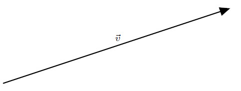
For the following two dimensional system, consider the vector, \(\boldsymbol{v}\):

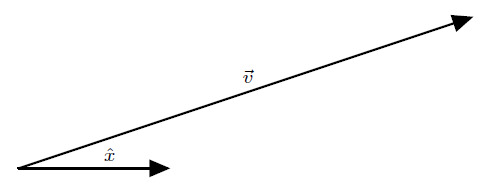
The most basic coordinate system is the Cartesian coordinate system. It’s also the most easily defined coordinate system. First, define one direction, called the \(x\) direction, by placing a vector, called \(\hat{x}\) (said aloud as “x hat”), in that direction:

Second, define a second direction that is perpendicular to the first, called the \(y\) direction, by placing a vector, called \(\hat{y}\), in that second direction. Both vectors should have the same length:

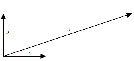
These two vectors, the coordinate vectors or basis vectors, are very special. As we have constructed, they define the two directions in space. They also define the fundamental length. In our system, we define the length of the coordinate vectors to be a length of \(1\) unit. Now that we have these two basis vectors, we can write the vector \(\boldsymbol{v}\) as a sum of the two basis vectors:

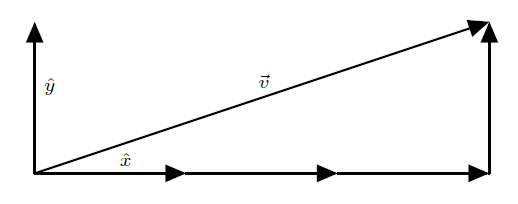
In this case, \[ \boldsymbol{v} = 3 \hat{x} + 1 \hat{y} \]

The numbers that we used in that sum, in this case, \(3\) and \(1\), are called the components of \(\boldsymbol{v}\). If everyone agrees on using this basis for describing the plane, we can do away with writing \(\boldsymbol{v}\) as this sum of basis vectors and instead refer to \(\boldsymbol{v}\) using just the components. In other words, we can write \[ \boldsymbol{v} = \left(3 ,1 \right) \]

This is usually how people learn how to write down vectors in high school. Now, here’s one subtlety that pervades our entire discussion of coordinate systems. I, again, emphasize that spatial vectors are geometric objects that are independent of the mathematical framework we build around them. Coordinate systems are one such mathematical framework. While the components of a vector refer to the vector, the vector is not the coordinates. Just writing down the list of numbers can be confusing! To make this clear, I could have defined our coordinate system differently. Suppose I defined it this way instead:

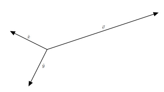
Now, the directions are completely different, and so are the lengths! The new components are (not surprisingly) completely different than the old components (for the curious, the new components are \( \left(-2, -2\right)\)). Nevertheless, these new components describe the same vector! The vector never changed, the coordinates did. To make things exactly clear what coordinate system you’re using, always draw your coordinate vectors in your diagrams. For clarity, I will usually write down vectors using the basis vectors rather than just the components.

One final point on the Cartesian system for completeness. Using the coordinate vectors, we can create a grid that can easily tell us what the coordinates of a point are:

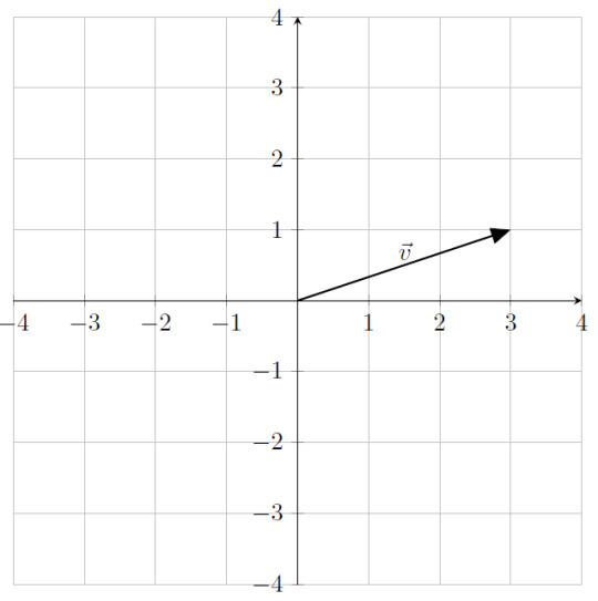
When a high school student thinks of “coordinates” or “coordinate system”, this grid is what they usually have in mind.

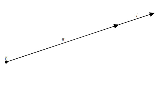
We can describe the same vector using a different coordinate system. This next system is the polar coordinate system. This system uses concentric circles to describe the position of any point. For two dimensions, we need to (again) define two pieces of information. First, we have to specify an origin point, \(\vec{0}\). This point is the center of the concentric circles and defines where the radius is zero. If we’re just describing a single vector, it is convenient to place the origin at the tail of the vector. By placing a unit vector that points radially outward, called \(\hat{r}\), we define the units of constant radius:

Second, we have to define some axis where we begin measuring angle:

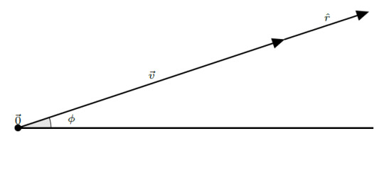
By convention, angle is measured increasing counterclockwise and is denoted by the Greek letter “phi”, \(\phi\). Once we have defined these two things, a radius and an angle, we can write any point on the plane using these two quantities. In this case, the point at the tip of \(\boldsymbol{v}\) can be written as the ordered pair \[ \left(r, \phi \right) = \left( 3.16, \frac{18.43}{180} \pi  \right) \]

(If you’re unfamiliar with using radians, using \(\pi\) to measure angles, don’t worry! I can cover that quickly later if there is demand.) This is great, but we would like to associate basis vectors with these quantities. We have already defined the radial basis vector, \(\hat{r}\). It points in the direction of increasing radius. We can define an angular basis vector, \(\hat{\phi}\), similarly. It points in the direction of increasing angle. Unlike the Cartesian coordinate system, though, these basis vectors aren’t so simple. The polar coordinate system (as well as many coordinate systems in general) is a system where the basis vectors are a function of position. Let’s see what this means. Consider the basis vectors at this point:

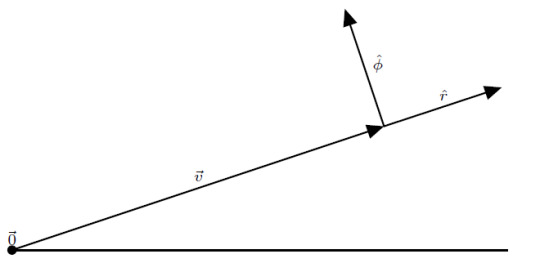
Now consider the basis vectors at this point:

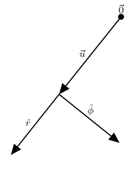
Just by changing what point we’re considering, the basis vectors have changed direction! The basis vectors depend on where you are. That’s because the concepts of “radially outward” and “direction of increasing angle” are different for different points on the plane. Radially outward is simply directly away from \(\vec{0}\), and the direction of increasing angle is perpendicular to the radially outward direction pointing in the counterclockwise direction. In other words, the directions of the polar basis vectors are locally defined.

Let’s look at one consequence of this. Suppose we are given the position vector of a moving particle \[ \boldsymbol{x}\left(t\right) = r \left(t\right) \hat{r} + \phi \left(t\right) \hat{\phi} \]

Suppose I ask you to calculate the velocity of this particle. The naive approach would be to say \[ \frac{d\boldsymbol{x}}{dt} = \frac{dr}{dt} \hat{r} + \frac{d\phi}{dt} \hat{\phi} \]

This would be wrong though. Since the basis vectors are themselves functions of position, we must differentiate them as well using the chain rule \[ \frac{d\boldsymbol{x}}{dt} = \frac{dr}{dt} \hat{r} + r \frac{d\hat{r}}{dt} + \frac{d\phi}{dt} \hat{\phi} + \frac{d\hat{\phi}}{dt} \]

Many physics problems are best described using circles, so when we discuss Newton’s Laws (which involve time derivatives) this complication will show up.

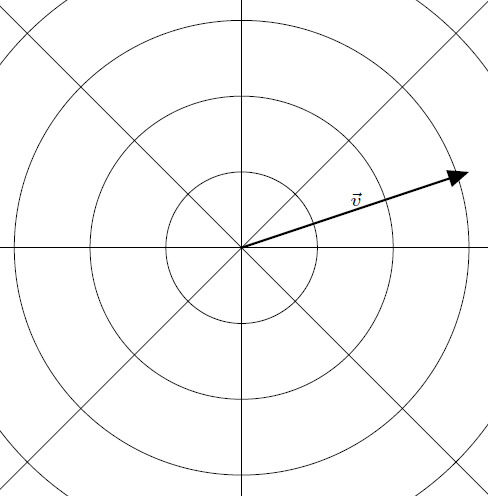
Finally, just like in the Cartesian system, we can define a similar “grid” for the polar system, but this time, we have circles of constant radius and lines of constant angle:

It is critical to note that for these two dimensional coordinate systems, we only needed two basis vectors to describe any point in the plane. That is to say, in two dimensions, we need two vectors to span the space. It shouldn’t surprise you that in three dimensions, we need three vectors to span the space. Let’s look at a few coordinate systems in three dimensions.

For the Cartesian coordinate system, the generalization is straightforward. Simply find a direction that is perpendicular to the two existing directions, then place another basis vector (usually called \(\hat{z}\)) in that direction.

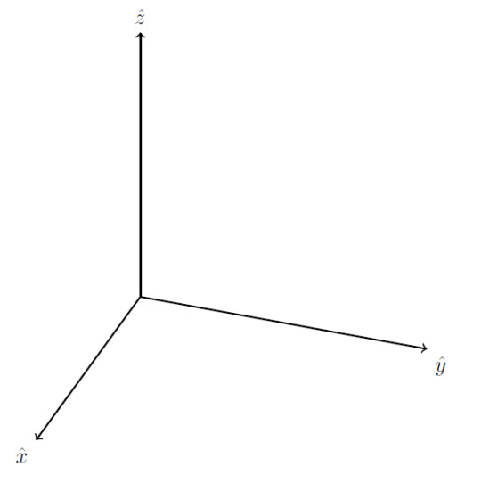
With that minor adjustment, you’re done. Except, not quite. You see, there is another direction that is perpendicular to the \(xy\) plane. We could have instead defined \(\hat{z}\) like this:

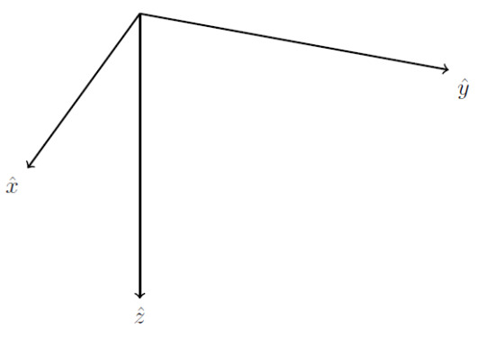
So which direction do we use? Technically, both answers are valid, but historically we have developed a convention to deal with this ambiguity. We demand that in three dimensions we use a right-handed coordinate system. What does this mean? This diagram (I shamelessly took from here) should explain:

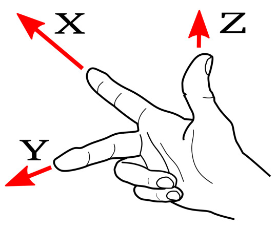
Take your right hand. Point your index finger in the \(\hat{x}\) direction. Point your middle finger perpendicular to your index finger so that it is in the \(\hat{y}\) direction. When you point your thumb up, this will be in the \(\hat{z}\) direction. I will explain why we choose right-handed systems in a little bit.

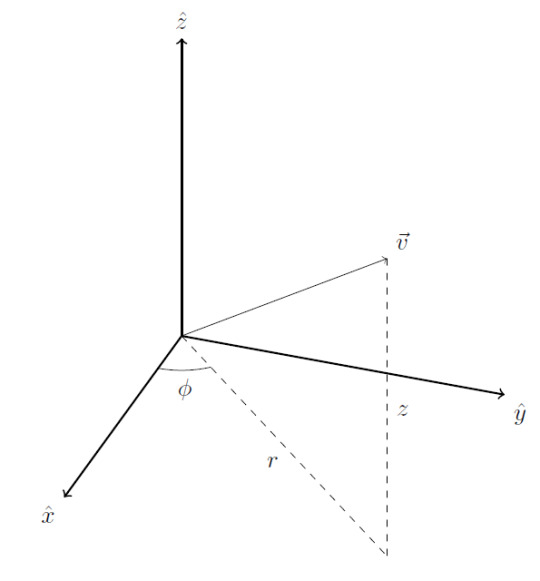
Generalizing polar coordinates is not as straightforward. There are two natural directions to go with this. We can keep the same two planar polar coordinates (radius and polar angle) and then specify which plane you’re on by using a \(\hat{z}\) coordinate. This gives us the cylindrical coordinate system:

We could also use a single radius and specify two angles (the polar and azimuthal angles typically). This gives us the spherical coordinate system:

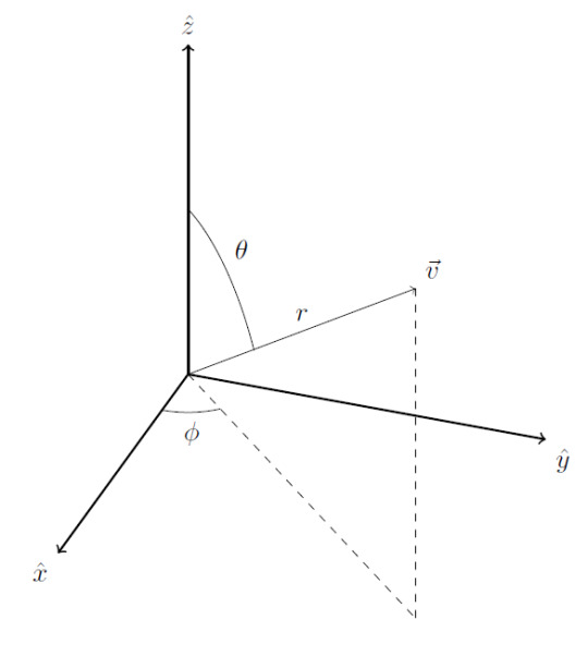
For both systems, the basis vectors (not pictured here) point in the direction of increasing coordinate. As with planar polar coordinates, these two polar coordinate systems have the disadvantage that their basis vectors aren’t constant.

Now that we know about coordinate systems, it becomes easy to talk about the two vector products. These two vector products are more mathematical framework that we introduce on top of vector arithmetic. One product will take two vectors and give us a number, while the other will take two vectors and give us a vector. Each product has a geometrical definition.

Consider two vectors, \(\boldsymbol{v}\) and \(\boldsymbol{w}\). Let the angle between them be denoted by \(\theta\). Also, let the length of \(\boldsymbol{v}\) and the length of \(\boldsymbol{w}\) be denoted by \(v\) and \(w\) respectively.

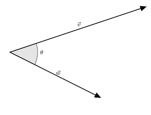
The dot product between two vectors, denoted \( \boldsymbol{v} \cdot \boldsymbol{w} \), is defined by multiplying the lengths of the two vectors with the cosine of the angle between them. That is to say, \[ \boldsymbol{v} \cdot \boldsymbol{w} = v w \cos\left(\theta\right) \]

Notice that the dot product of two vectors produces a scalar. That means it doesn’t make much sense to write down \( \boldsymbol{a} \cdot \boldsymbol{b} \cdot \boldsymbol{c} \) since you can’t take the dot product between a scalar and a vector.

Here’s a few properties of the dot product. Again, I’m stating these without proof (if you want the proofs please let me know!). If you take the dot product of a vector with itself, you get back the length of the vector squared \[ \boldsymbol{v} \cdot \boldsymbol{v} = v^2 \]

It doesn’t matter in what order you take the dot product \[ \boldsymbol{v} \cdot \boldsymbol{w} = \boldsymbol{w} \cdot \boldsymbol{v} \]

The dot product is distributive \[ \left( \boldsymbol{a} + \boldsymbol{b} \right) \cdot \boldsymbol{c} = \boldsymbol{a} \cdot \boldsymbol{c} + \boldsymbol{b} \cdot \boldsymbol{c} \]

The next few properties deal with that cosine in the definition. One consequence is that when two vectors are perpendicular, their dot product is zero since \(\cos\left(\frac{\pi}{2}\right)=0\).

Since the cosine of an angle is always between \(-1\) and \(1\), we get the Cauchy-Schwarz Inequality  \[ \left| \boldsymbol{v} \cdot \boldsymbol{w} \right| \leq \left|v\right| \left|w\right| \]

As a consequence of the Cauchy-Schwarz Inequality, we get the triangle inequality \[ \left| \boldsymbol{v} + \boldsymbol{w} \right| \leq \left|v\right| + \left| w \right| \]

Let’s think about what happens when we take dot products using our coordinate vectors. In Cartesian coordinates, our coordinate vectors are of unit length, and they are perpendicular to each other. This means their dot products are \[ \hat{x} \cdot \hat{y} = \hat{y} \cdot \hat{z} = \hat{z} \cdot \hat{x} = \cos\left(\frac{\pi}{2}\right) = 0 \]

Now, let’s see what happens when we take the dot product of two basis vectors with themselves. Again in Cartesian coordinates, \[ \hat{x} \cdot \hat{x} = \hat{y} \cdot \hat{y} = \hat{z} \cdot \hat{z} = \cos\left(0\right) = 1 \]

These two properties are given special names. When the dot product between two nonzero vectors is zero, we say those vectors are orthogonal. When a vector has unit length, it is said to be normalized. If the vectors in a basis are mutually orthogonal and are all normalized, the basis is said to be orthonormal. Orthonormality can be summed up in the statement \[ \hat{e}_i \cdot \hat{e}_j = \delta_{ij} \]

Where \(\delta_{ij} \) is the Kronecker delta symbol. The Kronecker delta is defined as \[\delta_{ij}=\begin{cases}1 & i=j\\\0 & \text{otherwise}\end{cases}\]

Orthonormality is not unique to the Cartesian basis. Since all of the bases I have described above have mutually orthogonal, normalized basis vectors, they are all orthonormal systems. Well, they are to some extent. Remember the business with the polar coordinate systems? Their basis vectors change with location. This has a subtle consequence. Consider the coordinate vector \(\hat{r}\left(\boldsymbol{r}\right) \) at two locations, \(\boldsymbol{r}=\boldsymbol{a}\) and \(\boldsymbol{r}=\boldsymbol{b}\). One would naively expect that \[ \hat{r}\left(\boldsymbol{a}\right) \cdot \hat{r}\left(\boldsymbol{b}\right) = 1 \]

But this is not the case! \(\hat{r}\left(\boldsymbol{a}\right)\) and \(\hat{r}\left(\boldsymbol{b}\right)\) could point in completely different directions, so it is not guaranteed that this inner product is \(1\). While the Cartesian system is globally orthonormal, the polar coordinate systems are only locally orthonormal. That means that statements like this are OK: \[ \hat{r}\left(\boldsymbol{a}\right) \cdot \hat{\theta}\left(\boldsymbol{a}\right) = \hat{\theta}\left(\boldsymbol{a}\right) \cdot \hat{\phi}\left(\boldsymbol{a}\right) = \hat{\phi}\left(\boldsymbol{a}\right) \cdot \hat{r}\left(\boldsymbol{a}\right) = 1 \]

But statements like this are BAD: \[ \hat{r}\left(\boldsymbol{a}\right) \cdot \hat{\theta}\left(\boldsymbol{b}\right) = \hat{\theta}\left(\boldsymbol{b}\right) \cdot \hat{\phi}\left(\boldsymbol{a}\right) = \hat{\phi}\left(\boldsymbol{a}\right) \cdot \hat{r}\left(\boldsymbol{a}\right) = 1 \]

As such, as is in many situations, it is often less confusing to convert from other coordinate systems back into Cartesian coordinates before performing many operations. So why is it easier to talk about the dot product now that we have coordinate systems? Well, in the Cartesian coordinate system, suppose we have two vectors written in terms of its components \[ \boldsymbol{v} = v_x \hat{x} + v_y \hat{y} + v_z \hat{z} \]

\[ \boldsymbol{w} = w_x \hat{x} + w_y \hat{y} + w_z \hat{z} \]

Let’s compute their dot product. We can write the vectors in terms of their components \[ \boldsymbol{v} \cdot \boldsymbol{w} = \left(v_x \hat{x} + v_y \hat{y} + v_z \hat{z}\right) \cdot \left(w_x \hat{x} + w_y \hat{y} + w_z \hat{z}\right) \]

Since the dot product is distributive, we can distribute this out into nine terms. However, since the basis is orthonormal, the cross terms (terms where things like \( \hat{x}\cdot\hat{y} \) appear) will become zero. What we’re left with is \[ \boldsymbol{v} \cdot \boldsymbol{w} = v_x w_x + v_y w_y + v_z w_z \]

If we have the Cartesian components of each vector, then the dot product becomes very easy to compute. The dot product allows us to do one more thing, though. It actually gives us a recipe to get those components! Suppose we don’t know the components of \( \boldsymbol{v} \), and we want to write it as \[ \boldsymbol{v} = v_x \hat{x} + v_y \hat{y} + v_z \hat{z} \]

To find any component we can exploit orthonormality. To find the \(\hat{x}\) component, take the dot product with \(\hat{x}\): \[ \boldsymbol{v} \cdot \hat{x} = v_x \]

The definition of the dot product says that this product should be \[ \boldsymbol{v} \cdot \hat{x} = v \cos\left(\theta\right) \]

Where \(\theta\) is the angle between \(\boldsymbol{v}\) and \(\hat{x}\). Since these are both the same dot product, they must be equal \[v_x = v \cos\left(\theta\right) \]

We can do this with the other basis vectors to find the other components. This operation, finding the length of one vector in the direction of another, is called projection.

One final remark about the dot product before we move on. The dot product is one of a larger class of operations called inner products. Inner products are defined for more general vectors (the mathematician’s definition of vectors), but many of the properties are similar. In fact, I tend to define orthogonality more generally than I just did above. If the inner product between two nonzero vectors is zero, they are orthogonal. When defining orthogonality this way, it liberates the inner product from any sense of geometry or angle. When discussing more general mathematical vectors, it doesn’t make as much sense to talk about the “angle” between two vectors and I think that trying to do so is misleading (looking at you Griffiths!). I will definitely come back to talk about inner products in their own dedicated essay.

Let’s define the other vector product. This will make clear why we chose right-handed coordinate systems. The vector cross product takes two vectors and returns another vector. Before I talk about how it’s defined and how to calculate it, I want to say a few general remarks about the cross product. First, the cross product only makes sense in three dimensions. There exists no two dimensional version of the cross product. If you go to higher than three dimensions, the cross product (or at least the operation that looks like the cross product) produces a tensor (a more complicated object) rather than a vector. Second, while the dot product is part of a larger collection of operations, the cross product is not. Finally, the cross product doesn’t always produce actual vectors. Instead, it sometimes produces pseudovectors, or axial vectors. I won’t go into much detail on what these things are until much later. Even though the output of the cross product isn’t a “real” vector in a sense, for brevity I will still call the cross product’s result a vector.

Let’s look at how to compute the cross product. The cross product between two vectors, denoted by \( \boldsymbol{v} \times \boldsymbol{w} \), is given by doing two things. Since the output of the cross product is a vector, we have to provide a method of getting the size and the direction of that vector. The size of the new vector is defined similarly to the dot product \[ \left| \boldsymbol{v} \times \boldsymbol{w} \right| = v w \sin\left(\theta\right) \]

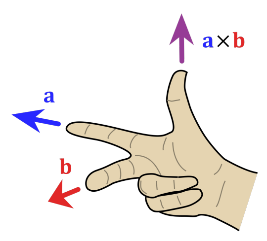
Then, the direction of the new vector is perpendicular to the plane of the original two vectors. Here, the same confusion arises as before with defining the coordinate systems. Which perpendicular direction should be used? Again, the answer is given by the right hand rule. This diagram (which I shamelessly stole from here), shows what to do:

I will only highlight three properties of the cross product. First, due to the sine in the definition, the length of the cross product is maximum when the two vectors are perpendicular, and the cross product is zero if both vectors point in either the same direction or in opposite directions. 

Second, due to the right hand rule, the cross product is anticommutative \[ \boldsymbol{v} \times \boldsymbol{w} = - \boldsymbol{w} \times \boldsymbol{v} \]

Finally, the cross product, like the dot product, is distributive \[ \left(\boldsymbol{a} + \boldsymbol{b} \right) \times \boldsymbol{c} = \boldsymbol{a} \times \boldsymbol{c} + \boldsymbol{b} \times \boldsymbol{c} \]

Again, let’s think of what happens when we take the cross product of coordinate vectors. This will explain why we choose right-handed systems. In the Cartesian system, \(\hat{x}\) and \(\hat{y}\) are perpendicular to each other and are of unit length. This means that \[ \left| \hat{x} \times \hat{y} \right| = 1 \]

When we use the right hand rule to find the direction of the cross product, we find that it points in the \(\hat{z}\) direction. This means that \[ \hat{x} \times \hat{y} = \hat{z} \]

A pretty cool result, no? Doing this for the other basis vectors produces a similar pattern \[ \hat{y} \times \hat{z} = \hat{x} \]

\[ \hat{z} \times \hat{x} = \hat{y} \]

Flip the order, you get a minus sign from anticommutativity. This pattern is called cyclic permittivity. This property, again, isn’t unique to the Cartesian system. Any right-handed coordinate system will allow you to locally cross two directions into the third direction.

Now, if you have two vectors written in terms of Cartesian components, \[ \boldsymbol{v} = v_x \hat{x} + v_y \hat{y} + v_z \hat{z} \]

\[ \boldsymbol{w} = w_x \hat{x} + w_y \hat{y} + w_z \hat{z} \]

Since the cross product is distributive, we could write down the components, distribute, figure out how the basis vectors cross into each other, and then write out the new vector. I leave this as an exercise to the reader to actually do this painful task. Fortunately, doing this once with these general components will reveal a general pattern for the components of the resulting vector. In practice people usually compute the cross product by computing the following determinant \[ \boldsymbol{v}\times\boldsymbol{w}=\left|\begin{array}{ccc} \hat{x} & \hat{y} & \hat{z}\\\ v_{x} & v_{y} & v_{z}\\\ w_{x} & w_{y} & w_{z} \end{array}\right| \]

When we calculate this determinant, this is equivalent to doing the entire distribution. It gives the following formula for the cross product: \[\boldsymbol{v}\times\boldsymbol{w}=\left(v_{y}w_{z}-w_{y}v_{z}\right)\hat{x}+\left(w_{x}v_{z}-v_{x}w_{z}\right)\hat{y}+\left(v_{x}w_{y}-w_{x}v_{y}\right)\hat{z}\]

One final remark about the vector products is that calculus still works on them. Suppose the vectors, \(\boldsymbol{v}\) and \(\boldsymbol{w}\), are both functions of time. Taking the time derivative of either product still invokes the product rule \[ \frac{d}{dt} \left( \boldsymbol{v} \cdot \boldsymbol{w} \right) = \frac{d \boldsymbol{v} }{dt} \cdot \boldsymbol{w} + \boldsymbol{v} \cdot \frac{d \boldsymbol{w} }{dt} \]

\[ \frac{d}{dt} \left( \boldsymbol{v} \times \boldsymbol{w} \right) = \frac{d \boldsymbol{v} }{dt} \times \boldsymbol{w} + \boldsymbol{v} \times \frac{d \boldsymbol{w} }{dt} \]

Now that we have coordinate systems under our belts, we can set up a problem, describe the geometry using a coordinate system, then work exclusively in components. These components will generalize into the concept of coordinates which I will develop in the next essay.

[onblogg]

On Spatial Vectors

There are a few more pieces of mathematical framework that we need to build before we can tackle the classical description of motion. These are the concepts of vectors and coordinates. I will discuss vectors here, and coordinates in the next two essays.

A vector consists of two pieces of information: a size and a direction. For instance, since it has some length and a direction in space, this arrow is a vector:

Vectors are physical objects that exist in space and time, independent of whatever framework we build around them. This is different from what a mathematician (or a computer scientist) would tell you. To a mathematician, a vector is a much more general mathematical object, which is a bit more complicated to talk about (to give you an idea of what we’d be getting into, to a mathematician, a vector is an element of a vector space... yikes!). I won’t discuss this general notion of vectors here. These special types of vectors, which can be represented using arrows, are called spatial vectors. Throughout my discussion of classical motion, whenever I discuss to vectors, I will be referring to these spatial vectors. 

As per usual in mathematics, it is helpful if we give the objects we discuss names. When writing the name of a vector, we type it in either boldface, \(\boldsymbol{v}\), or we write it with a small arrow on top, \(\vec{v}\). Consider two vectors, \(\boldsymbol{v}\) and \(\boldsymbol{w}\). We can do many operations using vectors. Since vectors are geometric objects, we don’t have to refer to any numbers to do arithmetic with them. Instead, all of the rules will be defined geometrically. The sum of \(\boldsymbol{v}\) and \(\boldsymbol{w}\), written as \(\boldsymbol{v} + \boldsymbol{w}\), is given by placing the tail of one vector onto the tip of the other:

Notice that it doesn’t matter if I place \(\boldsymbol{v}\) onto the tip of \(\boldsymbol{w}\) or if I place \(\boldsymbol{w}\) onto the tip of \(\boldsymbol{v}\):

You can scale the length of a vector by multiplying by a number (also known as a scalar since it “scales” the length):

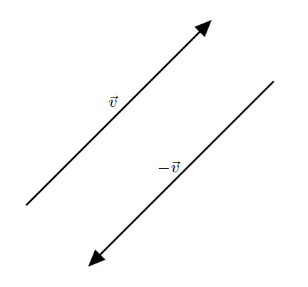
If you multiply by a negative number, it reverses the direction:

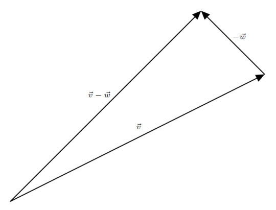
Subtraction is the same as adding the opposite, that is to say \[ \boldsymbol{v} - \boldsymbol{w} = \boldsymbol{v} + \left( - \boldsymbol{w} \right) \]

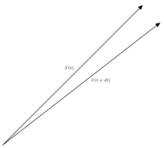
Vectors are useful for representing many different quantities. Consider this vector, \(\boldsymbol{s}\left(t\right)\):

It represents the distance from you to a passing car. Since the car moves, its position changes, and thus the vector also changes. This vector changes both its size and direction with time:

We can think of this vector as a function of time. This function, \(\boldsymbol{s}\left(t\right)\), takes a moment in time and maps it to some position in space. Vectors like this, called position vectors, are extremely important as we will come to see. Since this vector changes in time, we can do some calculus with it. Consider \(\boldsymbol{s}\left(t\right)\) at some time \(t\) and at some later time \(t + dt\):

Consider the difference between these two position vectors \[ \boldsymbol{s} \left(t + dt\right) - \boldsymbol{s} \left(t\right)\]

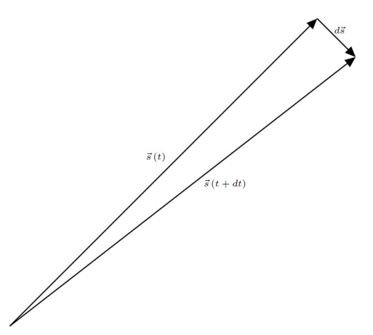
This infinitesimally small vector is the infinitesimal displacement \( d\boldsymbol{s} \). That is to say, \[ \boldsymbol{s} \left(t + dt\right) - \boldsymbol{s} \left(t\right) = d\boldsymbol{s} \].

Now, there’s a couple of things we can do now that we have this infinitesimal. Since we have defined addition of vectors, integration of vectors is possible since integration is just a special kind of sum. If we want to know the total displacement of the car, we can integrate over all \(d\boldsymbol{s}\), that is to say \[ \boldsymbol{S} = \int d\boldsymbol{s} \].

In addition, since we can multiply (and hence, divide) by numbers, we can do some differential calculus. Let’s consider dividing both sides of our equation for \( d\boldsymbol{s} \) by the infinitesimal time interval \(dt\). \[ \frac{ \boldsymbol{s} \left(t + dt\right) - \boldsymbol{s} \left(t\right) } {dt} = \frac{ d\boldsymbol{s} } { dt } \]

This should remind you of our definition of the derivative. What we have found by doing this division is the instantaneous velocity of the car. We can write this relation as \[ \boldsymbol{v} \left(t\right) = \frac{d\boldsymbol{s}}{dt} \]

With the instantaneous velocity (which is also a function of time), we can do the exact same analysis again to find the instantaneous acceleration. In fact, all of our work developing kinematics remains largely the same if we promote our one-dimensional position and acceleration to a vector position and acceleration \[ \frac{d^2 \boldsymbol{x} } {dt^2} = \boldsymbol{a} \]

So far, I have talked about spatial vectors in a very abstract sense. In principle, you can talk about all of the math we can do with spatial vectors without having to introduce any numbers to describe the vectors. In practice, however, it is convenient to define some system to describe vectors using numbers. To do so, you have to define a coordinate system. I will discuss coordinate systems in the next essay.

[onblogg]

On Infinitesimals

Before we return to our ball problem, I need to introduce the other half of calculus. This side also deals with the infinitesimally small, but for a vastly different purpose. This aside may seem like a waste of time at first, but it will turn out that this subject will be of fundamental importance to us.

Suppose I gave you an arbitrary curve. I (very rudely) demand that you tell me the area between this curve and the \(x\) axis from \(x = a\) to \(x=b\).

Make no mistake, this is a hard problem. Really, all areas we can calculate by hand are the areas of rectangles (OK, well, we have formulae for the areas of circles and circular objects, but without calculus, the layman probably could not come up with those formulae!). Let’s think about some basic shapes. We define area through rectangles, it’s just the width multiplied by the height:

This rectangle has width \(w\) and height \(h\), so the area of this rectangle is given by \[\text{area} = w \cdot h \]

The next basic shape is the triangle, which we can get by slicing a rectangle down the diagonal:

This slices the rectangle into two pieces. Each piece is a right triangle (a triangle with a right angle) which has exactly half of the area of the original rectangle, so the area of a right triangle is given by \[\text{area} = \frac{1}{2} w \cdot h \]

To find the area of a general triangle, we can split any triangle into right triangles:

The total area of this general triangle is just the sum of the two right triangles. Once we know the area of a triangle and a rectangle, we can readily find the area of any polygon. Suppose our polygon looked like this:

We can always decompose any polygon into many triangles.

To find the area of this polygon, we just need to split the polygon into triangles, find the area of the triangles, then add all of the areas up.

This is all well and good, but how does that help with our present problem? This curve is not a polygon. It twists, it doesn’t have sharp edges, it’s, well, a curve. Nevertheless, we can deal with this! To do so, we will have to make an approximation. Often in physics, it is helpful to create a brutalized model of whatever we’re trying to study so that we can gather a little intuition before tackling more accurate models. Here, we’re going to brutalize by approximating the area with a series of rectangles. The rule I’m going to follow is that the height of the rectangle will be given by the value of the function at the left endpoint:

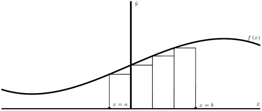
Notice how I chose the rectangles so that their widths are all equal. Suppose that width is \(w = \Delta x\). The area of each rectangle is simply the width times the height. Since I chose the height of the rectangle to be the value of \(f\) at the left endpoint, the area of each rectangle is given by \[ \text{area} = f\left( \text{left point} \right) \cdot \Delta x\]

The total area is then approximated by adding up all of the areas of the rectangles. Using this method, we undershoot the area a little bit. This is OK, though. We can improve this approximation by using more rectangles. In order to fit more rectangles into this interval, though, we would have to make them thinner. As we add more and more rectangles, we can get closer and closer to the actual area of the curve, that is to say, the error in our approximation will keep decreasing. Let’s cut to the chase. I want to approximate the area using a large number of thin rectangles. In this limit, there is no error in our approximation and our calculation of the area will be exact. Consider a rectangle of width \(dx\):

The left endpoint of this rectangle is at \(x = x\), and the right endpoint is at \( x = x + dx \) so that the width of the rectangle is \(dx\). As our name suggests, we are considering an infinitesimally thin rectangle. This thin rectangle has an infinitesimal area, \(dA\). Using our same left endpoint rule, this area is given by \[ dA = f\left(x\right) \cdot dx \]

Now, here is where we introduce our other piece of calculus. We know the infinitesimal area of each infinitesimally thin rectangle. How do we find the total area then? The exact same way as before! We just have to add up all of the infinitesimal areas. However, notice that there are an infinite number of infinitesimally thin rectangles to add. This kind of sum occurs so often that there is a special notation for it. When we add an infinite number of infinitesimally small things, we call it an integral. The total area is given by the integral of the infinitesimally small areas \[ A = \int dA \]

Plugging in for our above expression, we can find the total area underneath our curve. To denote that we are adding rectangles from \(x = a\) to \(x = b\), we write those values on our integral symbol. \[ A = \int dA = \int_{a}^{b} f\left(x\right) \, dx\]

This is all good notation, but I haven’t actually told you how to actually compute this area. So now, let us unite differential and integral calculus into the whole mathematics that is calculus. Let’s look back at our expression for the differential area. If we divide through by \(dx\), look at what we get: \[ \frac{dA}{dx} = f\left(x\right) \]

This should remind you of what we saw last time. There exists some function, \( A\left(x\right) \), which describes the area under the curve. The derivative of that area function is our original function that describes our curve. So the area function is precisely the antiderivative of the function describing the curve. The integral that I’ve described above, a definite integral, can be evaluated in the following way: find an antiderivative for the integrand (the function inside the integral), then plug in the value we wrote on the top of the integral (the upper limit) into the antiderivative, finally, plug in the value we wrote on the bottom of the integral (the lower limit) into the antiderivative and subtract the two values. Here’s a quick example to show what I mean.

We want to find the area underneath the parabola \( f\left(x\right) = x^2\) between \(x = 1\) and \(x=2\). The integral is written as \[ \int_{1}^{2} x^2 \, dx \]

An antiderivative for \(x^2\) is \(\frac{1}{3} x^3\). We can evaluate the integral \[ \int_{1}^{2} x^2 \, dx = \left[ \frac{1}{3} x^3 \right]_{1}^{2} \]

\[ \left[ \frac{1}{3} x^3 \right]_{1}^{2} = \frac{1}{3} \left(2\right)^3 - \left( \frac{1}{3} \left(1\right)^3 \right) = \frac{8}{3} - \frac{1}{3} = \frac{7}{3} \]

Notice that when we evaluate a definite integral, the result is a number. The variable of integration, which in this case was \(x\), is a dummy variable. I could have chosen to call this variable anything I wanted. To be explicit, \[ \int_{1}^{2} x^2 \, dx = \int_{1}^{2} \alpha^2 \, d\alpha = \int_{1}^{2} t^2 \, dt = \int_{1}^{2} \xi^2 \, d\xi   \]

To get a function that we can work with, we have to do something slightly different. We can generalize from the definite integral to get a function out the other end. We’ll let our lower limit be some number \(x_{0} \), and our upper limit be some other value \(x\). \[ A = \int_{x_{0}}^{x} f\left(x’\right) \, dx’\]

When I let the upper limit be a variable (which usually has the same name as the variable of integration), I will denote the variable of integration with a “prime”, in this case, \(x’\) (pronounced “x prime”). This is just to make sure that I know the difference between what’s a dummy variable (one that is integrated over) and what will be a “live” variable (the variable in our resulting function). Let’s suppose we know an antiderivative for \(f\left(x\right) \). Let’s call it \(F\left(x\right) \). Our area function will be given by evaluating the integral at both limits \[A\left(x\right) = \int_{x_{0}}^{x} f\left(x’\right) \, dx’ = F\left(x\right) - F\left(x_{0} \right) \]

Notice that with this, we now have a recipe for fixing that arbitrary constant! To do so, we need one additional piece of information. This is the value of \(F\) at \(x_{0}\).

OK. We have just covered a lot of concepts in a little time. Let me recap some things for you. We started with trying to find the area under a curve. We solve this problem by introducing the integral, a sum of infinitely many, infinitesimally small quantities. To actually evaluate the integral, we saw that the solution is given by the antiderivative of the function describing the curve. Finally, by letting the upper limit of integration be arbitrary, we could find the area function and solve for the arbitrary constant using some additional information. There are two concepts here that don’t have names yet. Let’s name them now.

We saw that we could solve the following equation using integration. \[ \frac{dA}{dx} = f\left(x\right) \]

This is an example of a differential equation. Differential equations are vitally important to physics, as we will come to see. Solutions to differential equations are functions, not numbers. The highest derivative of the differential equation determines the order of the equation. The above equation is a first order differential equation. If we are only supplied with this differential equation and no other information, we will be able to solve up to an arbitrary constant, as we have seen. Without additional information, solving a differential equation will give a family of functions, which differ from each other only in the arbitrary constant. Usually, the problem will give the necessary information to solve for the constant. Often, this information is of great physical significance. If we are integrating over time, this extra information is called the initial conditions. If we are integrating over space, this extra information is called the boundary conditions.

Finally, after all of that work, we can make sense of our falling ball. We have this second order differential equation \[ \frac{d^2 x}{dt^2} = a\left(t\right) \]

Remember Galileo’s observation? He tells us that \( a\left(t\right) = -g\), where \(g\) is a constant. We can write the differential equation as \[ \frac{d^2 x}{dt^2} = -g \]

First things first. We need to solve for the velocity, then solve for the position. Recall that \[ \frac{d^2 x}{dt^2} = \frac{dv}{dt} \]

We can solve this first order equation for velocity by integrating \[ dv = -g \,dt \]

\[ v\left(t\right) = \int_{t_{0}}^{t} -g \, dt’ \]

Since \(g\) is a constant, we can find the antiderivative readily \[ v\left(t\right) = \left[ -g t’ \right]_{t_{0}}^{t} = -gt + g t_{0} \]

Remember that \(v\) is the derivative of \(x\), which is what we really want to solve for. We have a second differential equation to solve now, \[ \frac{dx}{dt} = -gt + g t_{0} \]

We can also integrate to solve this \[ dx = \left(-gt + g t_{0} \right) \, dt \]

\[ x\left(t\right) = \int_{t_{0}}^{t} \left(-gt’ + g t_{0} \right) \, dt’ \]

Again, since this is a polynomial, we can find the antiderivative readily \[x\left(t\right) = \left[ -\frac{1}{2} g t’^2 + g t_{0} t’ \right]_{t_{0}}^{t} \]

\[x\left(t\right) = -\frac{1}{2} g t^2 + g t_{0} t + \frac{1}{2} g t_{0}^{2} - g t_{0}^{2} \]

\[x\left(t\right) = -\frac{1}{2} g t^2 + g t_{0} t - \frac{1}{2} g t_{0}^{2} \]

Notice that when we solved this second order equation, we have two arbitrary constants. The first constant, \( g t_{0} \), is the speed of the ball at time \( t = t_{0} \). Often, this speed is called \(v_{0}\). The second constant, \( \frac{1}{2} g t_{0}^2 \), is the position of the ball at time \( t = t_{0} \). Often, this position is called \(x_{0} \). As with many arbitrary constants, we usually absorb the minus sign into them. We can plug these numbers into our expression for the position to get \[x\left(t\right) = -\frac{1}{2} g t^2 + v_{0} t + x_{0} \]

These are the two initial conditions that need to be specified if we want to calculate a specific trajectory. Fortunately, we were told these initial conditions in the original problem statement. We wanted to find the trajectory of a ball that was dropped from rest. Without loss of generality, we can let the moment the ball was dropped be \(t = 0\). Since we were told that the ball was dropped from rest, it must have been at rest at \(t=0\). This means that its velocity was zero at \(t=0\), so to find \(v_{0}\), we have to look to our velocity function and solve the equation \[ v\left(0\right) = 0 \]

\[ 0 = -g \left(0\right) +v_{0} \]

\[ v_{0} = 0 \]

We can plug in this value to simplify our position function \[x\left(t\right) = -\frac{1}{2} g t^2 + x_{0} \]

In addition, we can define our coordinate system so that the ball’s initial position was \(x = 0\). We therefore need to solve the equation \[ x\left(0\right) = 0 \]

\[ x_{0} = 0 \]

Plugging this in, we can write down our position function. \[ x\left(t\right) = -\frac{1}{2} g t^2 \]

Notice, however, that I haven’t specified what the value of \left(g\right) is. This exact same analysis works for any body moving under constant acceleration. Studying the motion of bodies under constant acceleration is called kinematics, and the entirety of kinematics is beautifully and succinctly written in a single differential equation \[ \frac{d^2 x}{dt^2} = a \]

All of the kinematic equations that you see in a high-school level physics course come from this single relation. The rest of the so-called SUVAT formulae are obtained by eliminating variables when solving this differential equation.

So now, we have analyzed the hill alone and the ball alone. For completeness, we would want to be able to analyze the ball’s motion down the hill. For that, we will need some more mathematical machinery, and (finally!) some discussion of physical principles.

[onblogg]

On the Rules of Differentials and Antiderivatives

I will not prove any of these statements. If there is any interest, I can prove them later. For now, I just want to state the rules that I will be using henceforth. To make things clear, I will be taking derivatives of some functions, \(f\) and \(g\), which depend on a parameter, \(x\), which also depends on a parameter, \(t\). We can write the function \(f\) most generally as \(f\left(x\left(t\right)\right)\). In addition, I will be considering some numbers that I am calling \(a\) and \(b\). Here are some basic rules of the derivative:

The derivative is linear \[ \frac{d}{dx} \left( a f\left(x\right) + b g\left(x\right)\right) = a \frac{df}{dx} + b \frac{dg}{dx} \]

The derivative of a product of functions is given by the product rule \[ \frac{d}{dx} \left( f\left(x\right) \cdot g\left(x\right) \right) = \frac{df}{dx} \cdot g\left(x\right) + f\left(x\right) \cdot \frac{dg}{dx} \]

So far, we have taken derivatives with respect to \(x\). If we want to take the derivative of \(f\) with respect to \(t\), since \(x\) depends on \(t\), we have to use the chain rule \[ \frac{d}{dt} \left( f\left(x\left(t\right)\right)\right) = \frac{df}{dx} \cdot \frac{dx}{dt} \]

Finally, I will show explicitly the derivative of a power. Suppose \(f\left(x\right) = x^n\). The derivative of this function with respect to \(x\) is given by the power rule \[ \frac{d}{dx} \left( x^n \right) = n x^{\left(n-1\right)} \]

Using these rules, let’s look at a simple example: the derivative of a polynomial. Suppose \[ f\left(x\right) = 5x^4 + 2x^3 + \frac{1}{3} x^2 + x + 7 \]

We want to calculate \( \frac{df}{dx} \). Since the derivative is linear, we can act with the derivative on each of the terms individually and move the constants out front \[ \frac{df}{dx} = 5 \frac{d}{dx} \left(x^4\right) + 2 \frac{d}{dx} \left(x^3\right) + \frac{1}{3} \frac{d}{dx} \left(x^2\right) + \frac{d}{dx} \left(x\right) + \frac{d}{dx} \left(7\right) \]

We can evaluate the derivatives term by term now. I will only look at two of the terms. The rest should follow similarly. The first term is \[ 5 \frac{d}{dx} \left(x^4\right) \]

Using the power rule, this derivative evaluates to \[ 5 \cdot 4 x^{4-1} = 20 x^3\]

The other terms are calculated the same way. There is only one subtlety that should be pointed out. What should we do with the derivative of the constant term? That is to say, how do we calculate \[ \frac{d}{dx} \left( 7 \right) \]

I will argue this from two different angles. First, the algebraic argument. Recall that anything to the zeroth power is equal to one, that is to say \(x^0 = 1\). There is a power of \(x\) hiding in this constant expression, it’s just in the form \(x^0\). Once we include that power of \(x\) into the expression, we can evaluate the derivative easily \[ \frac{d}{dx} \left( 7 \right) = \frac{d}{dx} \left( 7 x^0 \right) = 7 \frac{d}{dx} \left(x^0\right) = 7 \cdot 0 x^{-1} = 0\]

The derivative of a constant is zero. This shouldn’t be mysterious at all, though! Here’s the intuitive argument. The derivative measures the rate of change with respect to some parameter. A constant, like \(7\), does not change if you vary any parameter. So the rate of change of \(7\) with respect to some parameter is zero since \(7\) doesn’t change. All that to say that the derivative of a constant is zero.

With these rules, we can guess at what the antiderivative of a polynomial must look like. If we were given \(f\left(x\right) =  x^2 \) for example, we know that the antiderivative must look something like \( F\left(x\right) = a x^3 \), where \(a\) is some constant that makes the following statement true \[ \frac{dF}{dx} = f\left(x\right) \]

That is to say, we can solve this equation to find the missing constant \[ \frac{d}{dx} \left( a x^3 \right) = x^2 \]

\[ 3ax^2 = x^2\]

\[3a = 1\]

\[a = \frac{1}{3}\]

So the antiderivative of \(f\) should be \( F\left(x\right) = \frac{1}{3} x^3 \), correct? WRONG. Well, sort of. You see, remember the whole business about taking the derivative of a constant? Well, since the derivative of a constant is zero, I could add any arbitrary constant to the antiderivative, and it would give the same derivative, so \[\begin{multline*}\frac{d}{dx} \left( \frac{1}{3} x^3 \right) = \frac{d}{dx} \left( \frac{1}{3} x^3 + 1 \right) =\\\\ \frac{d}{dx} \left( \frac{1}{3} x^3 + 25\right) = \frac{d}{dx} \left( \frac{1}{3} x^3 + 10^{26} \right) = x^2\end{multline*}\]

When taking antiderivatives, it is common to denote the arbitrary constant by \[ F\left(x\right) = \frac{1}{3} x^3 + C\]

But really, we can name these constants whatever we want, so often you will see them named after important quantities in the problem. Because, while the constants are arbitrary, in general, they can be determined by the problem. I’ll show you how to determine these arbitrary constants when we return to the problem of the falling ball next time.

[onblogg]

On Differentials

Calculus is intuitive for everyone. At least, it should be. The reason it isn’t is that we lock this knowledge behind over 10 years of formal mathematical training just to get a glimpse at its formal structure. It doesn’t have to be this way. Yes, a vast knowledge of algebra is very important for writing down and actually working with calculus. I don’t dispute that those years of mathematical training are required to completely understand calculus. Nevertheless, I believe that everyone can understand calculus at an intuitive level. Both aspects of calculus, differential and integral calculus, are geometric in nature. Anybody who has a simple grasp of geometry can understand what calculus does. While I will motivate calculus in this and the next essay, and I will readily use calculus henceforth, I will NOT be teaching calculus. One of my favorite YouTube channels, 3Blue1Brown, has an excellent and far superior introduction to calculus and its theorems. Instead, I will simply give some motivation and then launch into its applications.

Calculus is the mathematics of change. Differential calculus regards itself with calculating and quantifying change. What kinds of change? All quantifiable kinds of change! Let’s think of our hill and ball from last time. Not the ball yet, though, just the hill. Suppose the hill looked something like this:

We can ask about how the shape of the hill changes, that is, we can ask about its slope. Doing it is easy. We just measure how much the height changes over a certain amount of length:

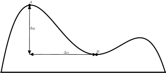
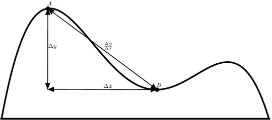
We can express this mathematically as \[ \text{slope} = \frac{\Delta y}{\Delta x} \] This is pretty good by itself, but it’s not calculus yet. There is one major issue with this current measurement. It’s an average. It doesn’t describe the entire hill very well. If we took the average here instead, we get a vastly different result:

In addition, this new result doesn’t describe the shape of this part of the hill too well. Luckily, there is a quick and easy way to get around this. We can take this average over a smaller distance a bunch of times to get different slope measurements for different parts of the hill:

It is now helpful to describe the height of the hill at each position using a function. This function eats a given position, \(x\), and spits out the height of the hill at that point, \(f\left(x\right)\). We can rewrite our expression for the slope using this notation. Suppose we measure the height at points \(x = a\) and \(x = b\). The average slope over this interval is given by \[ \frac{\Delta y}{\Delta x} = \frac{ f\left(b\right) - f\left(a\right) }{ b - a }\]

We don’t have to restrict ourselves to the interval between points \(a\) and \(b\). Instead, we will consider a general interval between some position \(x\) and another position ahead of \(x\), namely \(x + \delta x\).

Using these points, we can rewrite our expression for the slope as \[ \frac{\Delta y}{\Delta x} = \frac{ f\left( x + \delta x\right) - f\left(x\right) }{ \left(x + \delta x \right) - x} \]

Here’s where the calculus comes in. We can ask about the slope of increasingly smaller intervals. Formally, we express this as the limit where the interval length goes to zero. \[ \frac{dy}{dx} = \lim_{\delta x \rightarrow 0} \frac{ f\left(x + \delta x \right) - f\left(x\right) }{ \left(x + \delta x\right) - x} \]

In this limit, we know the slope of the curve at a single point. This difference quotient is the definition of the derivative. Why am I specifying that this is a limit? Let’s simplify the bottom of the fraction a little bit. \[ \frac{dy}{dx} = \lim_{\delta x \rightarrow 0} \frac{ f\left(x + \delta x \right) - f\left(x\right) }{ \delta x} \]

We see that if we were to let \(\delta x = 0\), we would be dividing by zero! That’s why I keep stressing that we’re considering a limit. We are not letting \(\delta x = 0\), we are looking at the behavior of this fraction as \(\delta x\) goes to zero. To see what this means, let’s zoom in on a small part of the hill:

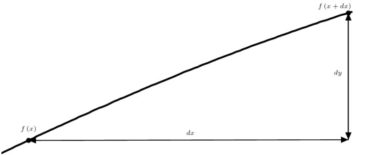
We consider an extremely small length, so small that we call it infinitesimal. Infinitesimals are extremely important in calculus. I will explain them in more detail next time. We use infinitesimal quantities so much in calculus that we denote them by placing a \(d\) in front of the quantity’s name. In this case, we call the infinitesimal distance \(dx\). We can then ask about the infinitesimal change in height, \(dy\), over the distance \(dx\). With these two quantities we can construct the local slope, and since these quantities are infinitesimally small, this is as good as taking the derivative. The slope, and hence the derivative, is given by \[\text{slope} = \frac{dy}{dx}\]

Now, I just did something that will deeply offend any mathematicians in the crowd (and will oust me immediately as a physicist). Although infinitesimals are such a useful concept, they aren’t mathematically rigorous. If we want to be fully rigorous with everything we do, we have to go back to the limit definition of the derivative. Nevertheless, outside of special cases that aren’t particularly physically important, using infinitesimals like I just did to build the derivative is effectively equivalent to using the formal definition, and I will be using this notion of infinitesimals throughout these essays since they are much more intuitive than using the formal definitions.

So we can find the slope of this hill wherever we want. So what? Well, this machinery that we just built, the derivative, is able to analyze all sorts of change. Let’s think about just the ball now. Suppose we were to drop the ball from rest in a vacuum under gravity. We want to quantify its motion to describe it. That means we want to know its position at every single moment in time. We have one piece of experimental evidence to help us along.

Galileo observed that all falling bodies fall with the same acceleration, regardless of their mass. How will this observation help us? How does acceleration mathematically relate to position? The answer (as you may expect by now) has to do with the derivative. Remember that derivatives measure change. But what exactly do they measure? With the hill, we were able to measure the slope of the hill at any point on it. The slope is the rate at which the height, \(y\), changed with respect to the length, \(x\). Derivatives tell us about change by quantifying the rate of change. Any motion has two extremely important rates of change. The first is the rate of change of position with respect to time. This is the velocity. The second rate is obtained from the velocity. It’s the rate of change of velocity with respect to time. This is the acceleration. Now we see where Galileo’s observation can help us. Mathematically, we can calculate the velocity by taking a derivative with respect to time, that is we can calculate \[ v = \frac{dx}{dt}\]

Similarly, we can calculate the acceleration by taking another time derivative \[ a = \frac{dv}{dt}\]

Notice, however, that since velocity is related to position, acceleration is also related to position \[ a = \frac{d}{dt} \left( \frac{dx}{dt} \right) \]

When we act with the same derivative twice, we say that we are calculating the second derivative. That is to say, acceleration is the second time derivative of position. We denote the second derivative more compactly as \[ a = \frac{ d^2 x}{dt^2} \]

More generally, if we have some quantity \(\alpha\) that changes with respect to some parameter \(s\), then we can take \(n\) derivatives with respect to \(s\) to find the rate of change, the rate of the rate of change, the rate of the rate of the rate of change, and so on. In particular, we denote the \(n\)th derivative by \[ \frac{ d^n \alpha}{ds^n}\]

So we now know how the acceleration of a body is related to its position. But that alone doesn’t help much at the moment. All we know is that the ball falls with constant acceleration. So far, all I have told you is how to go from knowing the position at every time to calculating the acceleration, not the other way around. For that, we need to how to start from the derivative and then recover the original function, that is to say, we need to know how to calculate an antiderivative. For this, we need to know how to take the derivative of simple functions, which I will discuss in the next essay.

[onblogg]

On the Classical Motion of Bodies

Try to build a description of motion from scratch. This is a very daunting task since there exists many kinds of motion and many things that move. If we assume nothing, we can’t say much about how stuff moves. It is unclear what rules, if any, motion follows. It is also unclear whether the same rules will apply to more than one object. To begin our description of motion, we have to make some assumptions and agree on some set of principles that we hold to be true. Fortunately, we don’t have to start from nothing. Our assumptions and principles can be informed by observation.

From personal experience, it is evident that some bodies follow somewhat predictable rules for how they move. Rocks fall. Wood falls. Water falls. A lot of bodies seem to fall towards the ground. To explain this common motion, it is simple to generalize from these individual observations. What is common between these objects? They are all… heavy. It is reasonable to guess that this rule will hold for all heavy bodies. That is to say, heavy bodies fall.

This revelation is great, but it hasn’t gotten us very far. This set of observations and this single generalization seems obvious to most people. Yet, this process is how many theories get started: start with some experimental evidence, then generalize so that you can explain all of the phenomena. But when these generalizations become more complicated, how can we know that they are correct?

There are two criteria that successful theories need to survive: agreement with observation and self-consistency. Self-consistency just means that the theory doesn’t contradict itself. Agreement with observation is a bit more subtle. Obviously our generalization needs to match what we have already observed, otherwise it wouldn’t be a good generalization. However, if the theory predicts any additional observable phenomena, then we must be able to observe those predictions. Let’s see if our heavy-body generalization fits these criteria. Is this generalization self-consistent? Since this generalization only makes one prediction, that heavy bodies fall, there isn’t much room for self-contradiction. Does this generalization match observation? Well, we can observe bodies that are definitely heavy, like birds and feathers, which do appear to rise, but always end up falling after some time. So far, so good. Water is a heavy body, so what happens to things placed into water? Some heavy bodies, like boulders, will continue to fall when placed into water. Others, like wood, cease to fall and float on top of the water. So heavy bodies float sometimes? This simple generalization does not explain that nor does it provide any prediction for this phenomenon. While our current description explains something about heavy bodies, it clearly isn’t the only principle governing falling bodies. So this description is incomplete. To further generalize, we have to take new observations and find new generalization that incorporates these new findings. So we return to the process of observing and generalizing.

I would love to continue this exercise, but our current approach to motion can only get us so far. This method of reasoning, through ordinary sensory experience alone, will ultimately lead us, as it did Aristotle, to an incorrect description of the world. To develop a more accurate model of motion, we have to turn to the tools that astronomers have used for centuries and what Galileo realized was necessary to fully and precisely describe motion: idealization and mathematics.

Why would idealization be useful for finding more accurate descriptions of motion? By removing many realistic elements of the situations we describe, wouldn’t that severely limit the application of our generalization? It is precisely because of this stripping-down of the problem that we can generate more powerful generalizations.

Consider a simple problem. A solid ball is placed on a hill and allowed to roll down under gravity. What elements of this problem are truly important, and what can be safely ignored to solve it? Let’s think of some things that may or may not severely affect the motion. Gravity is obviously important, since it’s what accelerates the ball. How about the air around the ball? If the ball doesn’t move very fast, then air resistance doesn’t play a significant role. Since the ball rolls only under the force of gravity, if the hill in question isn’t too tall (say, a few meters or so) so that the ball never goes too fast, we can treat this situation as if there were no air at all without losing much accuracy. How about any deformation of the hill or the ball? If both the ball and the hill are stiff enough, that is they don’t deform under the weight of the ball, these effects can also be safely ignored.

So we have come across two classic idealizations commonly used in classical problems: ignoring air resistance (placing the setup in a vacuum) and rigid bodies. Obviously, these idealizations are not realistic. Rarely on the Earth do we encounter a vacuum nor do we have balls and hills that are perfectly rigid, but these idealizations allow us to isolate the essence of the problem. Once we understand this simple model, it isn’t too hard to go back and refine the model by adding nonidealities back in. In fact, many problems are tackled in this way. We consider toy models that may seem extremely contrived, but end up giving us immense understanding of the underlying physics.

With how much work and wordiness this essay has been to this point, it should be clear that English is a pretty inefficient way to describe physical situations. If describing the problem using words is this hard, just think about how hard it must be to give adequate explanations of the underlying physics! Luckily, we have a better way of providing these descriptions and explanations. Unfortunately, is akin to another language entirely. Many people, in fact, recoil in disgust and fear when the even think of it! That is, of course, the language of mathematics. Once we accept that we can idealize physical situations to better understand them, we can begin to apply mathematics to these situations. Mathematics allows us to quantify our physical situations and our motion. We can now discuss precisely distances traveled over certain periods of time as well as other measurements. We can use all of the powerful theorems Euclid and others developed for geometry, as well as the powerful theorems regarding algebra. And with the help of Descartes, we can unite the two and fully describe any physical situation using analytical geometry.

It is a large philosophical debate whether or not mathematical descriptions are another form of idealization. After all, the objects in geometry are themselves ideal. Perfect circles simply do not exist in our universe. Do our mathematical theories truly represent reality as it is or do they only represent some contrived idealized reality? For now, I will ignore this point since our theories and models simply would not exist if it weren’t for the underlying math.

To completely describe motion, we need a particular kind of mathematics. Motion, at its core, is a kind of change. The study of motion, therefore, is a study of change. So to completely and mathematically describe motion, we must first understand the mathematics of change. This mathematics, the Calculus, is credited to Newton and Leibniz. And it is Calculus that I will explore in the next essay.

[onblogg]

On Motion

At the most basic level, Physics is the study of motion. This statement is deceptively simple. Learning how and why bodies move led to the development of advanced mathematics, unthinkably complex technologies, and various mind-bending theories that have completely reshaped our ideas of space, time, and determinism. How could a study of motion have led to all of this? That is what this series of essays will be about.

Why study motion? What motivates humanity to find precisely how bodies move? Many human issues stem from or are solved by motion. The motion of bodies, such as a thrown spear, matters a lot when your survival depends on it. Whether for hunting, agriculture, construction, or war, humans have always needed to move within their environment or move something around them to survive. It would be nice to know precisely how an arrow flies so that your family always has a meal, or so that the opposing archer doesn’t have a chance to fire back at you.

The motion of water has always dictated human life in some way. From the regular flooding of the Nile, to supplying Los Angeles via aqueducts, much care has been taken to understand and control the motion of water. To the ancient Egyptians, the motion of the Nile seemed to be controlled by the motion of another set of bodies. These bodies were not found on the ground, and could only be seen during the night. Indeed, the motion of the stars through the night sky over the course of the year allowed the Egyptians to predict the flooding of the Nile. Egypt, like many other cultures around the world, used Astronomy to tell when to plant and when to harvest, which would facilitate the rise of civilizations.

Understanding another kind of flow would cause another monumentous revolution. Although the motion of electrically charged bodies began as a mere curiosity, humanity’s attempts to understand the flow of electricity would lead to the modern world, where the flow of electricity is a necessity for daily life. Understanding this kind of motion is necessary for understanding modern life.

Needless to say, studying motion is important for understanding our past, present, and future. More importantly, motion is a kind of change. In our quest to understand motion, we will develop many skills and techniques to precisely describe and explain it. We will be able to apply those same skills and techniques to better understand change in general. And we will begin to learn about those skills and techniques in the next essay.

[onblogg]

On Blogging

This blog will be an experimental personal project in honing my technical writing skills. I expect to post some material every week, though its length and quality will vary. I have not determined what subjects I want to write about, but expect many of the subjects to be somewhat technical (i.e., expect \(math\)). To communicate my ideas effectively, I will be using extensive use of \(\LaTeX\) whenever necessary. 

I hope you will enjoy my ramblings.