peevalue

[peevalue]

Module 8 - ANOVA

Code for question 1:

> # Data > stress_high <- c(10, 9, 8, 9, 10, 8) > stress_med <- c(8, 10, 6, 7, 8, 8) > stress_low <- c(4, 6, 6, 4, 2, 2) > > stress_data <- data.frame(stress_low, stress_med, stress_high) > stress_stack <- stack(stress_data) > > # Perform one-way test > oneway.test(values ~ ind, data = stress_stack)

One-way analysis of means (not assuming equal variances)

data:  values and ind F = 17.525, num df = 2.0000, denom df = 9.2777, p-value = 0.0007065

> > # Perform ANOVA test > aov_results <- aov(values ~ ind, data = stress_stack) > summary(aov_results)            Df Sum Sq Mean Sq F value   Pr(>F)     ind          2  82.11   41.06   21.36 4.08e-05 *** Residuals   15  28.83    1.92                     --- Signif. codes:  0 ‘***’ 0.001 ‘**’ 0.01 ‘*’ 0.05 ‘.’ 0.1 ‘ ’ 1

---------------------------------------------------

Question 2:  From our Textbook:Introductory Statistics with R. Chapter # 6 Exercises 6.1 pp. 127 plus. The zelazo data (taken from textbook's R package called ISwR) are in the form of a list of vectors, one for each of the four groups. Convert the data to a form suitable for the user of lm, and calculate the relevant test. Consider t tests comparing selected subgroups or obtained by combing groups.     2.1  Consider ANOVA test (one way or two-way) to this dataset (zelazo)

> library("ISwR") > data("zelazo") > > # Convert Zelazo data into data frame > zelazo_df <- as.data.frame(matrix(unlist(zelazo), nrow=6)) Warning message: In matrix(unlist(zelazo), nrow = 6) :  data length [23] is not a sub-multiple or multiple of the number of rows [6] > colnames(zelazo_df) <- c("active", "passive", "none", "ctr.8w") > > zelazo_stack <- stack(zelazo_df) > > # Delete incorrect value in entry 6 of ctr.8w > zelazo_stack[[24, 1]] = NA > > # Perform ANOVA test > anova_zelazo <- aov(values ~ ind, data = zelazo_stack) > summary(anova_zelazo)                    Df     Sum Sq   Mean Sq   F value   Pr(>F) ind                3     14.78       4.926        2.142      0.129 Residuals   19     43.69       2.299               1 observation deleted due to missingness

[peevalue]

Module 7 - Regression Analysis

1.)

x <- c(16, 17, 13, 18, 12, 14, 19, 11, 11, 10) y <- c(63, 81, 56, 91, 47, 57, 76, 72, 62, 48)

1.1 Define the relationship model between the predictor and the response variable:

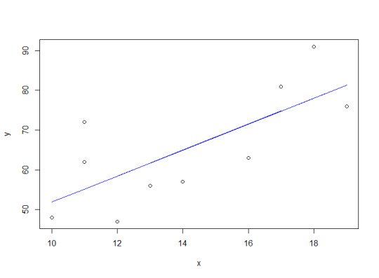
plot(x, y) linear_model <- lm(y ~ x) lines(x, fitted(linear_model), col="blue")

As shown by the blue line representing the linear model, the relationship between the predictor and response variable appears linear with a positive slope.

1.2 Calculate the coefficients? > print(linear_model) Call: lm(formula = y ~ x) Coefficients: (Intercept)            x       19.206        3.269  

Using the lm() function, the coefficients 19.206 for the intercept and 3.269 for x are returned.

2.) Apply the simple linear regression model (see the above formula) for the data set called "visit" (see below), and estimate the the discharge duration if the waiting time since the last eruption has been 80 minutes.

> head(visit)  discharge  waiting 1     3.600      79 2     1.800      54 3     3.333      74 4     2.283      62 5     4.533      85 6     2.883      55

Employ the following formula discharge ~ waiting and data=visit)

2.1 Define the relationship model between the predictor and the response variable.

discharge <- c(3.6, 1.8, 3.333, 2.283, 4.533, 2.883) waiting <- c(79, 54, 74, 62, 85, 55) linear_model2 <- lm(discharge ~ waiting) print(linear_model2) plot(waiting, discharge) lines(waiting, fitted(linear_model2), col="blue")

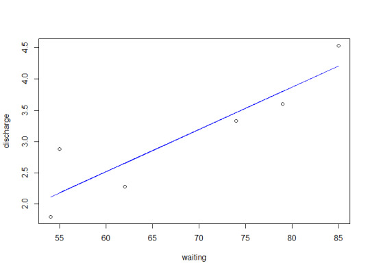
As shown in the plot above, the model is linear with a positive slope. 2.2 Extract the parameters of the estimated regression equation with the coefficients function.

> coeffs <- coef(linear_model2) > estimate <- coeffs[1] + coeffs[2] * 80 # Y = a + bX where a is intercept (X = 0), b = slope, x = 80 > estimate (Intercept)   3.871431

According to this calculation using the formula Y = a + bX, we can expect the discharge time to be approximately 3.87 when the waiting time is equal to 80.

2.3 Determine the fit of the eruption duration using the estimated regression equation.

The fit can be seen above in the line on the plot.

3.) Multiple Regression

3.1 Examine the relationship Multi Regression Model as stated above and its Coefficients using 4 different variables from mtcars (mpg, disp, hp and wt). Report on the result and explanation what does the multi regression model and coefficients tells about the data?  

> linear_model3

Call: lm(formula = mpg ~ disp + hp + wt, data = input)

Coefficients: (Intercept)         disp           hp           wt    37.105505    -0.000937    -0.031157    -3.800891

According to the output of the lm function, it seems that mpg and (disp, hp, wt) are inversely related. Cars with high mpg have low disp, hp, and/or wt.

4.)  From our textbook pp. 110 Exercises # 5.1 With the rmr data set, plot metabolic rate versus body weight. Fit a linear regression to the relation. According to the fitted model, what is the predicted metabolic rate for a body weight of 70 kg?

> library(ISwR) > plot(metabolic.rate ~ body.weight,data=rmr) > linear_model4 <- lm(metabolic.rate ~ body.weight, data=rmr)

> linear_model4 Call: lm(formula = metabolic.rate ~ body.weight, data = rmr) Coefficients: (Intercept)  body.weight       811.23         7.06   > coeffs2 <- coef(linear_model4) > estimate2 <- coeffs2[1] + coeffs2[2] * 70 > estimate2 (Intercept)   1305.394

Using this code, we can see that the estimated metabolic rate for a body weight of 70 kg would be 1305.394

[peevalue]

Module 6 - Random Variable(s) & Probability Distribution(s) and and One-sample and Two sample Tests

A. Consider a population consisting of the following values, which represents the number of ice cream purchases during the academic year for each of the five housemates. 8, 14, 16, 10, 11

1.) Compute the mean of this population. Population mean = 11.8

2.) Select a random sample of size 2 out of the five members. I created a function to create a data frame that creates ‘x’ samples of n=2 and calculates mean, standard deviation, and compares the sample mean and standard deviation to the population mean and standard deviation. Here is the data frame:

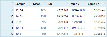
3.) Compute the mean and standard deviation of your sample. See above data frame.

4.) Compare the Mean and Standard deviation of your sample to the entire population of this set (8,14, 16, 10, 11). Population mean = 11.8, random sample 1 mean = 12.5 Population s = 3.19, random sample 1 s = 2.12

B. Suppose that the sample size n = 100 and the population proportion p = 0.95.

1.) Does the sample proportion p have approximately a normal distribution? Explain. The sample proportion p has an approximately normal distribution. If n*p >= 5 and n*q >= 5, then the distribution is expected to be normal.

2.) What is the smallest value of n for which the sampling distribution of p is approximately normal?   n*(0.95) = 5 5 / 0.95 =  5.26

n*(0.05) = 5 5 / 0.05 = 100

Therefore, the smallest value of n for which the sampling distribution of p is approximately normal is n = 100.

C. Simulated coin-tossing is probably better done using rbinom than using sample. Explain how

The sample function simply returns a vector of randomly selected values from X which would require more work to analyze the results. Whereas rbinom will return multiple values containing the results of multiple sets of trials.

> sample(c("H", "T"), 10, replace=TRUE) [1] "H" "T" "T" "T" "T" "T" "T" "T" "H" "T" - Not that useful

> rbinom(10, 100, 0.5) [1] 58 51 48 51 52 51 48 46 49 46 - Much more useful

[peevalue]

Module 5 - Hypothesis Testing and Correlation Analysis

First Question:

The director of manufacturing at a cookies needs to determine whether a new machine is production a particular type of cookies according to the manufacturer's specifications, which indicate that cookies should have a mean of 70 and standard deviation of 3.5 pounds. A sample pf 49 of cookies reveals a sample mean breaking strength of 69.1 pounds.

A. State the null and alternative hypothesis: Null Hypothesis:  μ =  μ0 Alternative Hypothesis:  μ <=  μ0

B. Is there evidence that the machine is nor meeting the manufacturer's specifications for average strength? Use a 0.05 level of significance: p(0.04) < alpha(0.05); The evidence shows that the machine is not meeting the manufacturer's specification of 70 pounds.

C. Compute the p value and interpret its meaning p-value = 0.0359. This is the probability of a type-I error occurring. This value is less than alpha, so it suggests that the null hypothesis should be rejected.

D. What would be your answer in (B) if the standard deviation were specified as 1.75 pounds? p(0.0002) < alpha(0.05); The evidence shows that the machine is not meeting the manufacturer's specification of 70 pounds.

E. What would be your answer in (B) if the sample mean were 69 pounds and the standard deviation is 3.5 pounds? p(0.0228) < alpha(0.05); The evidence shows that the machine is not meeting the manufacturer's specification of 70 pounds.

Second Question:

If x̅ = 85, σ = standard deviation = 8, and n=64, set up 95% confidence interval estimate of the population mean μ.

95% CI for μ = (83.04, 86.96)

Third Question: 

NOTE: THE PROVIDED DATA AND INSTRUCTIONS DID NOT MAKE SENSE. INSTEAD, I AM MAKING MY OWN CORRELATION BETWEEN THE TIME SPENT STUDYING FOR BOYS AND GIRLS (x) AND GRADES FOR BOYS AND GIRLS (y). THE DATA IS AS FOLLOWS:

x <- c(19, 22, 28, 18.9, 22.2, 27.8) # Time spent studying for boys and girls y <- c(49, 50, 69, 46.1, 54.2, 67.7) # Grades for boys and girls

a. Calculate the correlation coefficient for this data set Using the formula: (r) =[ nΣxy – (Σx)(Σy) / Sqrt([nΣx2 – (Σx)2][nΣy2 – (Σy)2])] (converted to R code): r = (6 * sum(x * y) - (sum(x) * sum(y))) / sqrt((6 * sum(x)*2 - sum(x)*2) * (6 * sum(y)*2 - sum(y)*2)),

r = 0.55

b. Pearson correlation coefficient Using cor(x, y, method=“pearson”) r = 0.98

c. Create plot of the correlation

Scatter plot-

correlogram - Pearson

correlogram - Spearman

[peevalue]

Module 4 - Probability Theory

A:

A1.) P(A) = 10 + 20 = 30

A2.) P(B) = 10 + 20 = 30

A3.) P(A or B) (not mutually exclusive) = 30 + 30 - 10 = 50

A4.) P(A or B) (mutually exclusive) = P(A) + P(B) = 30 + 30 = 60

B - What is the probability that it will rain on Jane’s wedding day: Jane is getting married tomorrow, at an outdoor ceremony in the desert. In recent years, it has rained only 5 days each year. Unfortunately, the weatherman has predicted rain for tomorrow. When it actually rains, the weatherman correctly forecasts rain 90% of the time. When it doesn't rain, he incorrectly forecasts rain 10% of the time.

Solution: The sample space is defined by two mutually-exclusive events - it rains or it does not rain. Additionally, a third event occurs when the weatherman predicts rain. Notation for these events appears below.

Event A1. It rains on Jane's wedding. Event A2. It does not rain on Jane’s wedding. Event B. The weatherman predicts rain. In terms of probabilities, we know the following: P( A1 ) = 5/365 =0.0136985 [It rains 5 days out of the year.] P( A2 ) = 360/365 = 0.9863014 [It does not rain 360 days out of the year.] P( B | A1 ) = 0.9 [When it rains, the weatherman predicts rain 90% of the time.] P( B | A2 ) = 0.1 [When it does not rain, the weatherman predicts rain 10% of the time.] We want to know P( A1 | B ), the probability it will rain on the day of Jane’s wedding, given a forecast for rain by the weatherman. The answer can be determined from Bayes' theorem, as shown below.

P( A1 | B ) = P( A1 ) P( B | A1 ) / P( A1 ) P( B | A1 ) + P( A2 ) P( B | A2 ) P( A1 | B ) = (0.014)(0.9) / [ (0.014)(0.9) + (0.986)(0.1) ] P( A1 | B ) = 0.111 Note the somewhat unintuitive result. Even when the weatherman predicts rain, it only rains only about 11% of the time. Despite the weatherman's gloomy prediction, there is a good chance that Marie will not get rained on at her wedding.

True or False?

Answer: This is true. Bayes' theorem has been applied correctly and the calculations are correct. 

Events A1 and A2 are mutually exclusive as it can only be raining or not raining on a given day. It only rains 5 days of the year, so P(A1) is 5/365 = 0.0136985. P(A2) is the inverse, resulting in 360/365 = 0.9863014.

P(B) given A1 is .9 because when it rains, the weatherman correctly predicted it the day before.

P(B) given A2 is .1 because when it does not rain, the weatherman incorrectly predicted it will rain the day before.

C. Last assignment from our textbook, pp. 55 Exercise # 2.3. For a disease known to have a postoperative complication frequency of 20%, a surgeon suggests a new procedure. She/he tests it on 10 patients and found there are not complications. What is the probability of operating on 10 patients successfully with the traditional method?

Result:

> dbinom(10, 10, .2) [1] 1.024e-07

The probability of successfully performing the traditional method 10 times consecutively is near zero. The new method is far superior to the old one.

[peevalue]

Module 3 - Descriptive Statistcs

Note: Since R does not have a function to get the statistical mode, I used this function by user Ken Williams on StackOverflow.  (https://stackoverflow.com/questions/2547402/how-to-find-the-statistical-mode).

I could have used traditional programming techniques like using a for-loop to iterate and count the occurrences of each value, but that didn’t seem very true to R-style programming.

Results:

The only difference between the descriptive statistics of the two sets are the central tendency measurements, which are the same measurements as set1, but 10 has been added to each value. This is because set2 is the same as set1 with 10 added to each element. Because the variance of all the elements of the two sets are equal, the variance measurements of both sets will be equal as well.

[peevalue]

Module 2 - myMean

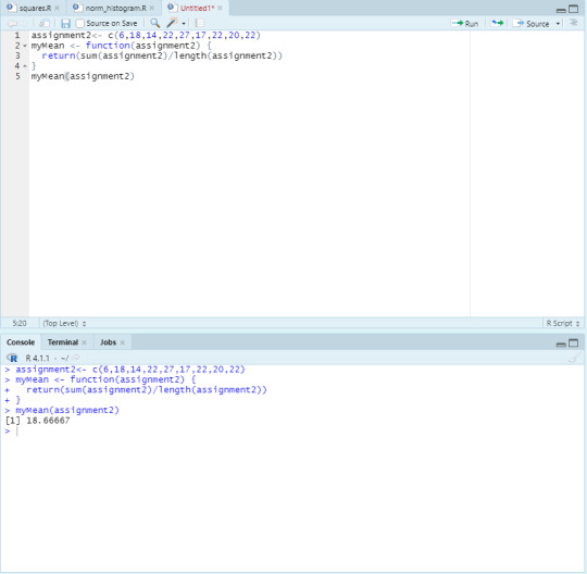
Here is a screenshot of the script containing the myMean function and its results.

First, we define assignment2 and use the c function to set assignment2 to a vector containing the values  6, 18, 14, 22, 27, 17, 22, 20, 22.

Then, we define myMean as a function which takes assignment2 as a parameter. The myMean function then returns the quotient of the sum of all of assignment2′s elements by the length of the assignment2 vector by using the sum and length functions.

The mean of the given data is 18.66667.