ramu3218

[ramu3218]

Running a k-means Cluster Analysis:

Machine Learning for Data Analysis

Week 4: Running a k-means Cluster Analysis

A k-means cluster analysis was conducted to identify underlying subgroups of countries based on their similarity of responses on 7 variables that represent characteristics that could have an impact on internet use rates. Clustering variables included quantitative variables measuring income per person, employment rate, female employment rate, polity score, alcohol consumption, life expectancy, and urban rate. All clustering variables were standardized to have a mean of 0 and a standard deviation of 1.

Because the GapMinder dataset which I am using is relatively small (N < 250), I have not split the data into test and training sets. A series of k-means cluster analyses were conducted on the training data specifying k=1-9 clusters, using Euclidean distance. The variance in the clustering variables that was accounted for by the clusters (r-square) was plotted for each of the nine cluster solutions in an elbow curve to provide guidance for choosing the number of clusters to interpret.

Load the data, set the variables to numeric, and clean the data of NA values

In [1]:''' Code for Peer-graded Assignments: Running a k-means Cluster Analysis Course: Data Management and Visualization Specialization: Data Analysis and Interpretation ''' import pandas as pd import numpy as np import matplotlib.pyplot as plt import statsmodels.formula.api as smf import statsmodels.stats.multicomp as multi from sklearn.cross_validation import train_test_split from sklearn import preprocessing from sklearn.cluster import KMeans data = pd.read_csv('c:/users/greg/desktop/gapminder.csv', low_memory=False) data['internetuserate'] = pd.to_numeric(data['internetuserate'], errors='coerce') data['incomeperperson'] = pd.to_numeric(data['incomeperperson'], errors='coerce') data['employrate'] = pd.to_numeric(data['employrate'], errors='coerce') data['femaleemployrate'] = pd.to_numeric(data['femaleemployrate'], errors='coerce') data['polityscore'] = pd.to_numeric(data['polityscore'], errors='coerce') data['alcconsumption'] = pd.to_numeric(data['alcconsumption'], errors='coerce') data['lifeexpectancy'] = pd.to_numeric(data['lifeexpectancy'], errors='coerce') data['urbanrate'] = pd.to_numeric(data['urbanrate'], errors='coerce') sub1 = data.copy() data_clean = sub1.dropna()

Subset the clustering variables

In [2]:cluster = data_clean[['incomeperperson','employrate','femaleemployrate','polityscore', 'alcconsumption', 'lifeexpectancy', 'urbanrate']] cluster.describe()

Out[2]:incomeperpersonemployratefemaleemployratepolityscorealcconsumptionlifeexpectancyurbanratecount150.000000150.000000150.000000150.000000150.000000150.000000150.000000mean6790.69585859.26133348.1006673.8933336.82173368.98198755.073200std9861.86832710.38046514.7809996.2489165.1219119.90879622.558074min103.77585734.90000212.400000-10.0000000.05000048.13200010.40000025%592.26959252.19999939.599998-1.7500002.56250062.46750036.41500050%2231.33485558.90000248.5499997.0000006.00000072.55850057.23000075%7222.63772165.00000055.7250009.00000010.05750076.06975071.565000max39972.35276883.19999783.30000310.00000023.01000083.394000100.000000

Standardize the clustering variables to have mean = 0 and standard deviation = 1

In [3]:clustervar=cluster.copy() clustervar['incomeperperson']=preprocessing.scale(clustervar['incomeperperson'].astype('float64')) clustervar['employrate']=preprocessing.scale(clustervar['employrate'].astype('float64')) clustervar['femaleemployrate']=preprocessing.scale(clustervar['femaleemployrate'].astype('float64')) clustervar['polityscore']=preprocessing.scale(clustervar['polityscore'].astype('float64')) clustervar['alcconsumption']=preprocessing.scale(clustervar['alcconsumption'].astype('float64')) clustervar['lifeexpectancy']=preprocessing.scale(clustervar['lifeexpectancy'].astype('float64')) clustervar['urbanrate']=preprocessing.scale(clustervar['urbanrate'].astype('float64'))

Split the data into train and test sets

In [4]:clus_train, clus_test = train_test_split(clustervar, test_size=.3, random_state=123)

Perform k-means cluster analysis for 1-9 clusters

In [5]:from scipy.spatial.distance import cdist clusters = range(1,10) meandist = [] for k in clusters: model = KMeans(n_clusters = k) model.fit(clus_train) clusassign = model.predict(clus_train) meandist.append(sum(np.min(cdist(clus_train, model.cluster_centers_, 'euclidean'), axis=1)) / clus_train.shape[0])

Plot average distance from observations from the cluster centroid to use the Elbow Method to identify number of clusters to choose

In [6]:plt.plot(clusters, meandist) plt.xlabel('Number of clusters') plt.ylabel('Average distance') plt.title('Selecting k with the Elbow Method') plt.show()

Interpret 3 cluster solution

In [7]:model3 = KMeans(n_clusters=4) model3.fit(clus_train) clusassign = model3.predict(clus_train)

Plot the clusters

In [8]:from sklearn.decomposition import PCA pca_2 = PCA(2) plt.figure() plot_columns = pca_2.fit_transform(clus_train) plt.scatter(x=plot_columns[:,0], y=plot_columns[:,1], c=model3.labels_,) plt.xlabel('Canonical variable 1') plt.ylabel('Canonical variable 2') plt.title('Scatterplot of Canonical Variables for 4 Clusters') plt.show()

Begin multiple steps to merge cluster assignment with clustering variables to examine cluster variable means by cluster.

Create a unique identifier variable from the index for the cluster training data to merge with the cluster assignment variable.

In [9]:clus_train.reset_index(level=0, inplace=True)

Create a list that has the new index variable

In [10]:cluslist = list(clus_train['index'])

Create a list of cluster assignments

In [11]:labels = list(model3.labels_)

Combine index variable list with cluster assignment list into a dictionary

In [12]:newlist = dict(zip(cluslist, labels)) print (newlist) {2: 1, 4: 2, 6: 0, 10: 0, 11: 3, 14: 2, 16: 3, 17: 0, 19: 2, 22: 2, 24: 3, 27: 3, 28: 2, 29: 2, 31: 2, 32: 0, 35: 2, 37: 3, 38: 2, 39: 3, 42: 2, 45: 2, 47: 1, 53: 3, 54: 3, 55: 1, 56: 3, 58: 2, 59: 3, 63: 0, 64: 0, 66: 3, 67: 2, 68: 3, 69: 0, 70: 2, 72: 3, 77: 3, 78: 2, 79: 2, 80: 3, 84: 3, 88: 1, 89: 1, 90: 0, 91: 0, 92: 0, 93: 3, 94: 0, 95: 1, 97: 2, 100: 0, 102: 2, 103: 2, 104: 3, 105: 1, 106: 2, 107: 2, 108: 1, 113: 3, 114: 2, 115: 2, 116: 3, 123: 3, 126: 3, 128: 3, 131: 2, 133: 3, 135: 2, 136: 0, 139: 0, 140: 3, 141: 2, 142: 3, 144: 0, 145: 1, 148: 3, 149: 2, 150: 3, 151: 3, 152: 3, 153: 3, 154: 3, 158: 3, 159: 3, 160: 2, 173: 0, 175: 3, 178: 3, 179: 0, 180: 3, 183: 2, 184: 0, 186: 1, 188: 2, 194: 3, 196: 1, 197: 2, 200: 3, 201: 1, 205: 2, 208: 2, 210: 1, 211: 2, 212: 2}

Convert newlist dictionary to a dataframe

In [13]:newclus = pd.DataFrame.from_dict(newlist, orient='index') newclus

Out[13]:0214260100113142163170192222243273282292312320352373382393422452471533543551563582593630......145114831492150315131523153315431583159316021730175317831790180318321840186118821943196119722003201120522082210121122122

105 rows × 1 columns

Rename the cluster assignment column

In [14]:newclus.columns = ['cluster']

Repeat previous steps for the cluster assignment variable

Create a unique identifier variable from the index for the cluster assignment dataframe to merge with cluster training data

In [15]:newclus.reset_index(level=0, inplace=True)

Merge the cluster assignment dataframe with the cluster training variable dataframe by the index variable

In [16]:merged_train = pd.merge(clus_train, newclus, on='index') merged_train.head(n=100)

Out[16]:indexincomeperpersonemployratefemaleemployratepolityscorealcconsumptionlifeexpectancyurbanratecluster0159-0.393486-0.0445910.3868770.0171271.843020-0.0160990.79024131196-0.146720-1.591112-1.7785290.498818-0.7447360.5059900.6052111270-0.6543650.5643511.0860520.659382-0.727105-0.481382-0.2247592329-0.6791572.3138522.3893690.3382550.554040-1.880471-1.9869992453-0.278924-0.634202-0.5159410.659382-0.1061220.4469570.62033335153-0.021869-1.020832-0.4073320.9805101.4904110.7233920.2778493635-0.6665191.1636281.004595-0.785693-0.715352-2.084304-0.7335932714-0.6341100.8543230.3733010.177691-1.303033-0.003846-1.24242828116-0.1633940.119726-0.3394510.338255-1.1659070.5304950.67993439126-0.630263-1.446126-0.3055100.6593823.1711790.033923-0.592152310123-0.163655-0.460219-0.8010420.980510-0.6448300.444628-0.560127311106-0.640452-0.2862350.1153530.659382-0.247166-2.104758-1.317152212142-0.635480-0.808186-0.7874660.0171271.155433-1.731823-0.29859331389-0.615980-2.113062-2.423400-0.625129-1.2442650.0060770.512695114160-0.6564731.9852172.199302-1.1068200.620643-1.371039-1.63383921556-0.430694-0.102586-0.2240530.659382-0.5547190.3254460.250272316180-0.559059-0.402224-0.6041870.338255-1.1776610.603401-1.777949317133-0.419521-1.668438-0.7331610.3382551.032020-0.659900-0.81098631831-0.618282-0.0155940.061048-1.2673840.211226-1.7590620.075026219171.801349-1.030498-0.4344840.6593820.7029191.1165791.8808550201450.447771-0.827517-1.731013-1.909640-1.1561120.4042250.7359771211000.974856-0.034925-0.0068330.6593822.4150301.1806761.173646022178-0.309804-1.755430-0.9368040.8199460.653945-1.6388680.2520513231732.6193200.3033760.217174-0.946256-1.0346581.2296851.99827802459-0.056177-0.2669040.2714790.8199462.0408730.5916550.63990432568-0.562821-0.3538960.0271070.338255-0.0316830.481486-0.1037773261080.111383-1.030498-1.690284-1.749076-1.3167450.5879080.999290127212-0.6582520.7286690.678765-0.464565-0.364702-1.781946-0.78874722819-0.6525281.1926250.6855540.498818-0.928876-1.306335-0.617060229188-0.662484-0.4505530.135717-1.106820-0.672255-0.147127-1.2726732..............................70140-0.594402-0.044591-0.8214060.819946-0.3157280.5125720.074137371148-0.0905570.052066-0.3190860.8199460.0936890.7235950.80625437211-0.4523170.1583900.549792-1.7490761.2768870.177913-0.140250373641.636776-0.779188-0.1697480.8199461.1084191.2715050.99128407484-0.117682-1.156153-0.5295180.9805101.8214720.5500380.5527263751750.604211-0.3248980.0882000.9805101.5903171.048938-0.287918376197-0.481087-0.0735890.393665-2.070203-0.356866-0.404628-0.287029277183-0.506714-0.808186-0.067926-2.070203-0.347071-2.051902-1.340281278210-0.628790-1.958410-1.887139-0.946256-1.297156-0.353290-1.08675317954-0.5150780.042400-0.1765360.1776910.5109430.6733710.467327380114-0.6661982.2945212.111056-0.625129-1.077755-0.229248-1.1365692814-0.5503841.5889211.445822-0.946256-0.245207-1.8114130.072358282911.575455-0.769523-0.1154430.980510-0.8426821.2795041.62732708377-0.5015740.332373-0.2783580.6593820.0545110.221758-0.28880838466-0.265535-0.0252600.305419-0.1434370.516820-0.6358011.332879385921.240375-1.243145-0.8349830.9805100.5677521.3035020.5785230862011.4545511.540592-0.733161-1.909640-1.2344700.7659211.014413187105-0.004485-1.281808-1.7513770.498818-0.8857790.3704051.418278188205-0.593947-0.1702460.305419-2.070203-0.629158-0.070373-0.8118762891540.504036-0.1605810.1696570.9805101.3846291.0649370.19511839045-0.6307520.061732-0.678856-0.625129-0.068902-1.377621-0.27991229197-0.6432031.3472771.2557550.498818-0.576267-1.199710-1.488839292632.067368-0.1992430.3597250.9805101.2298731.1133390.365916093211-0.6469130.1680550.3665130.498818-0.638953-2.020815-0.874146294158-0.422620-0.943506-0.2919340.8199461.8273490.505990-0.037060395135-0.6635950.2453810.4411820.338255-0.862272-0.018934-1.68276529679-0.6744750.6416770.1221410.338255-0.572349-2.111239-1.1223362971790.882197-0.653534-0.4344840.9805100.9810881.2578350.980609098149-0.6151691.0766361.4118810.017127-0.623282-0.626890-1.891814299113-0.464904-2.354706-1.4459120.8199460.4149550.5938830.5260393

100 rows × 9 columns

Cluster frequencies

In [17]:merged_train.cluster.value_counts()

Out[17]:3 39 2 35 0 18 1 13 Name: cluster, dtype: int64

Calculate clustering variable means by cluster

In [18]:clustergrp = merged_train.groupby('cluster').mean() print ("Clustering variable means by cluster") clustergrp Clustering variable means by cluster

Out[18]:indexincomeperpersonemployratefemaleemployratepolityscorealcconsumptionlifeexpectancyurbanratecluster093.5000001.846611-0.1960210.1010220.8110260.6785411.1956961.0784621117.461538-0.154556-1.117490-1.645378-1.069767-1.0827280.4395570.5086582100.657143-0.6282270.8551520.873487-0.583841-0.506473-1.034933-0.8963853107.512821-0.284648-0.424778-0.2000330.5317550.6146160.2302010.164805

Validate clusters in training data by examining cluster differences in internetuserate using ANOVA. First, merge internetuserate with clustering variables and cluster assignment data

In [19]:internetuserate_data = data_clean['internetuserate']

Split internetuserate data into train and test sets

In [20]:internetuserate_train, internetuserate_test = train_test_split(internetuserate_data, test_size=.3, random_state=123) internetuserate_train1=pd.DataFrame(internetuserate_train) internetuserate_train1.reset_index(level=0, inplace=True) merged_train_all=pd.merge(internetuserate_train1, merged_train, on='index') sub5 = merged_train_all[['internetuserate', 'cluster']].dropna()

In [21]:internetuserate_mod = smf.ols(formula='internetuserate ~ C(cluster)', data=sub5).fit() internetuserate_mod.summary()

Out[21]:

OLS Regression ResultsDep. Variable:internetuserateR-squared:0.679Model:OLSAdj. R-squared:0.669Method:Least SquaresF-statistic:71.17Date:Thu, 12 Jan 2017Prob (F-statistic):8.18e-25Time:20:59:17Log-Likelihood:-436.84No. Observations:105AIC:881.7Df Residuals:101BIC:892.3Df Model:3Covariance Type:nonrobustcoefstd errtP>|t|[95.0% Conf. Int.]Intercept75.20683.72720.1770.00067.813 82.601C(cluster)[T.1]-46.95175.756-8.1570.000-58.370 -35.534C(cluster)[T.2]-66.56684.587-14.5130.000-75.666 -57.468C(cluster)[T.3]-39.48604.506-8.7630.000-48.425 -30.547Omnibus:5.290Durbin-Watson:1.727Prob(Omnibus):0.071Jarque-Bera (JB):4.908Skew:0.387Prob(JB):0.0859Kurtosis:3.722Cond. No.5.90

Means for internetuserate by cluster

In [22]:m1= sub5.groupby('cluster').mean() m1

Out[22]:internetuseratecluster075.206753128.25501828.639961335.720760

Standard deviations for internetuserate by cluster

In [23]:m2= sub5.groupby('cluster').std() m2

Out[23]:internetuseratecluster014.093018121.75775228.399554319.057835

In [24]:mc1 = multi.MultiComparison(sub5['internetuserate'], sub5['cluster']) res1 = mc1.tukeyhsd() res1.summary()

Out[24]:

Multiple Comparison of Means - Tukey HSD,FWER=0.05group1group2meandifflowerupperreject01-46.9517-61.9887-31.9148True02-66.5668-78.5495-54.5841True03-39.486-51.2581-27.7139True12-19.6151-33.0335-6.1966True137.4657-5.76520.6965False2327.080817.461736.6999True

The elbow curve was inconclusive, suggesting that the 2, 4, 6, and 8-cluster solutions might be interpreted. The results above are for an interpretation of the 4-cluster solution.

In order to externally validate the clusters, an Analysis of Variance (ANOVA) was conducting to test for significant differences between the clusters on internet use rate. A tukey test was used for post hoc comparisons between the clusters. Results indicated significant differences between the clusters on internet use rate (F=71.17, p<.0001). The tukey post hoc comparisons showed significant differences between clusters on internet use rate, with the exception that clusters 0 and 2 were not significantly different from each other. Countries in cluster 1 had the highest internet use rate (mean=75.2, sd=14.1), and cluster 3 had the lowest internet use rate (mean=8.64, sd=8.40).

[ramu3218]

RUNNING A RASSO REGRESSION :

Machine Learning for Data Analysis

Week 3: Running a Lasso Regression Analysis

Continuing on the machine learning analysis of internet use rate from the GapMinder dataset, I conducted a lasso regression analysis to identify a subset of variables from a pool of 10 quantitative predictor variables that best predicted a quantitative response variable measuring the internet use rates of the countries in the world. I have added several variables to my standard analysis that are not particularly interesting to my main question of how internet use rates of a country affects income in order to have more variables available for this lasso regression. The explanatory variables I have used in this model are income per person, employment rate, female employment rate, polity score, alcohol consumption, life expectancy, oil per person, electricity use per person, and urban rate. All variables have been normalized to have a mean of zero and standard deviation of one.

Load the data, convert all variables to numeric, and discard NA values

In [1]:''' Code for Peer-graded Assignments: Running a Lasso Regression Analysis Course: Data Management and Visualization Specialization: Data Analysis and Interpretation ''' import pandas as pd import numpy as np import matplotlib.pyplot as plt from sklearn.cross_validation import train_test_split from sklearn.linear_model import LassoLarsCV data = pd.read_csv('c:/users/greg/desktop/gapminder.csv', low_memory=False) data['internetuserate'] = pd.to_numeric(data['internetuserate'], errors='coerce') data['incomeperperson'] = pd.to_numeric(data['incomeperperson'], errors='coerce') data['employrate'] = pd.to_numeric(data['employrate'], errors='coerce') data['femaleemployrate'] = pd.to_numeric(data['femaleemployrate'], errors='coerce') data['polityscore'] = pd.to_numeric(data['polityscore'], errors='coerce') data['alcconsumption'] = pd.to_numeric(data['alcconsumption'], errors='coerce') data['lifeexpectancy'] = pd.to_numeric(data['lifeexpectancy'], errors='coerce') data['oilperperson'] = pd.to_numeric(data['oilperperson'], errors='coerce') data['relectricperperson'] = pd.to_numeric(data['relectricperperson'], errors='coerce') data['urbanrate'] = pd.to_numeric(data['urbanrate'], errors='coerce') sub1 = data.copy() data_clean = sub1.dropna()

Select predictor variables and target variable as separate data sets

In [3]:predvar = data_clean[['incomeperperson','employrate','femaleemployrate','polityscore', 'alcconsumption', 'lifeexpectancy', 'oilperperson', 'relectricperperson', 'urbanrate']] target = data_clean.internetuserate

Standardize predictors to have mean = 0 and standard deviation = 1

In [4]:predictors=predvar.copy() from sklearn import preprocessing predictors['incomeperperson']=preprocessing.scale(predictors['incomeperperson'].astype('float64')) predictors['employrate']=preprocessing.scale(predictors['employrate'].astype('float64')) predictors['femaleemployrate']=preprocessing.scale(predictors['femaleemployrate'].astype('float64')) predictors['polityscore']=preprocessing.scale(predictors['polityscore'].astype('float64')) predictors['alcconsumption']=preprocessing.scale(predictors['alcconsumption'].astype('float64')) predictors['lifeexpectancy']=preprocessing.scale(predictors['lifeexpectancy'].astype('float64')) predictors['oilperperson']=preprocessing.scale(predictors['oilperperson'].astype('float64')) predictors['relectricperperson']=preprocessing.scale(predictors['relectricperperson'].astype('float64')) predictors['urbanrate']=preprocessing.scale(predictors['urbanrate'].astype('float64'))

Split data into train and test sets

In [6]:pred_train, pred_test, tar_train, tar_test = train_test_split(predictors, target, test_size=.3, random_state=123)

Specify the lasso regression model

In [7]:model=LassoLarsCV(cv=10, precompute=False).fit(pred_train,tar_train)

Print the regression coefficients

In [9]:dict(zip(predictors.columns, model.coef_))

Out[9]:{'alcconsumption': 6.2210718136158443, 'employrate': 0.0, 'femaleemployrate': 0.0, 'incomeperperson': 10.730391071065633, 'lifeexpectancy': 7.9415161171462634, 'oilperperson': 0.0, 'polityscore': 0.33239766774625268, 'relectricperperson': 3.3633566029800468, 'urbanrate': 1.1025066401058063}

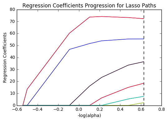
Plot coefficient progression

In [12]:m_log_alphas =-np.log10(model.alphas_) ax = plt.gca() plt.plot(m_log_alphas, model.coef_path_.T) plt.axvline(-np.log10(model.alpha_), linestyle='--', color='k', label='alpha CV') plt.ylabel('Regression Coefficients') plt.xlabel('-log(alpha)') plt.title('Regression Coefficients Progression for Lasso Paths') plt.show()

Plot mean square error for each fold

In [13]:m_log_alphascv =-np.log10(model.cv_alphas_) plt.figure() plt.plot(m_log_alphascv, model.cv_mse_path_, ':') plt.plot(m_log_alphascv, model.cv_mse_path_.mean(axis=-1), 'k', label='Average across the folds', linewidth=2) plt.axvline(-np.log10(model.alpha_), linestyle='--', color='k', label='alpha CV') plt.legend() plt.xlabel('-log(alpha)') plt.ylabel('Mean squared error') plt.title('Mean squared error on each fold') plt.show()

Print the mean squared error from training and test data

In [17]:from sklearn.metrics import mean_squared_error train_error = mean_squared_error(tar_train, model.predict(pred_train)) test_error = mean_squared_error(tar_test, model.predict(pred_test)) print ('training data MSE') print(train_error) print ('') print ('test data MSE') print(test_error) training data MSE 100.103936002 test data MSE 120.568970231

Print the r-squared from training and test data

In [18]:rsquared_train=model.score(pred_train,tar_train) rsquared_test=model.score(pred_test,tar_test) print ('training data R-square') print(rsquared_train) print ('') print ('test data R-square') print(rsquared_test) training data R-square 0.861344142378 test data R-square 0.776942580854

Data were randomly split into a training set that included 70% of the observations (N=42) and a test set that included 30% of the observations (N=18). The least angle regression algorithm with k=10 fold cross validation was used to estimate the lasso regression model in the training set, and the model was validated using the test set. The change in the cross validation average (mean) squared error at each step was used to identify the best subset of predictor variables.

Of the 10 predictor variables, 6 were retained in the model. During the estimation process, income per person and life expectancy were most strongly associated with internet use rate, followed by alcohol consumption and electricity use per person. The last two predictors were urban rate and polity score. All variables were positively correlated with internet use rate. These 6 variables accounted for 77.7% of the variance in the internet use rate response variable.

[ramu3218]

RUNNING A RANDOM FOREST:

Machine Learning for Data Analysis

Running a Random Forest

The main drawback to a decision tree is that the tree is highly specific to the dataset it was built on; if you bring in new data to try and predict outcomes, you may not find the same high correlations that your decision tree featured. One method to overcome this is with a random forest. Instead of building one tree from your whole dataset, you subset the data randomly and build a number of trees. Each tree will be different, but the relationships between your variables will tend to appear consistently. In general though, because decision trees are intrinsically connected to the specific data they were built with, decision trees are better as a tool to analyze trends within a known dataset than to create a model for predicting the outcomes of future data.

With those caveats, I decided to build a random forest using the same data as from my previous post, that is, a response variable of internet use rate and explanatory variables of income per person, employment rate, female employment rate, and polity score, from the GapMinder dataset.

Load the data, convert the variables to numeric, convert the response variable to binary, and remove NA values.

In [3]:''' Code for Peer-graded Assignments: Running a Random Forest Course: Data Management and Visualization Specialization: Data Analysis and Interpretation ''' import pandas as pd import numpy as np import matplotlib.pyplot as plt from sklearn.cross_validation import train_test_split import sklearn.metrics from sklearn.ensemble import ExtraTreesClassifier data = pd.read_csv('c:/users/greg/desktop/gapminder.csv', low_memory=False) data['internetuserate'] = pd.to_numeric(data['internetuserate'], errors='coerce') data['incomeperperson'] = pd.to_numeric(data['incomeperperson'], errors='coerce') data['employrate'] = pd.to_numeric(data['employrate'], errors='coerce') data['femaleemployrate'] = pd.to_numeric(data['femaleemployrate'], errors='coerce') data['polityscore'] = pd.to_numeric(data['polityscore'], errors='coerce') binarydata = data.copy() # convert response variable to binarydef internetgrp (row): if row['internetuserate'] < data['internetuserate'].median(): return 0 else: return 1 binarydata['internetuserate'] = binarydata.apply (lambda row: internetgrp (row),axis=1) # Clean the dataset binarydata_clean = binarydata.dropna()

Build the model from the training set

In [10]:predictors = binarydata_clean[['incomeperperson','employrate','femaleemployrate','polityscore']] targets = binarydata_clean.internetuserate pred_train, pred_test, tar_train, tar_test = train_test_split(predictors, targets, test_size=.4) from sklearn.ensemble import RandomForestClassifier classifier_r=RandomForestClassifier(n_estimators=25) classifier_r=classifier_r.fit(pred_train,tar_train) predictions_r=classifier_r.predict(pred_test)

Print the confusion matrix

In [11]:sklearn.metrics.confusion_matrix(tar_test,predictions_r)

Out[11]:array([[22, 5], [10, 24]])

Print the accuracy score

In [12]:sklearn.metrics.accuracy_score(tar_test, predictions_r)

Out[12]:0.75409836065573765

Fit an Extra Trees model to the data

In [13]:model_r = ExtraTreesClassifier() model_r.fit(pred_train,tar_train)

Out[13]:ExtraTreesClassifier(bootstrap=False, class_weight=None, criterion='gini', max_depth=None, max_features='auto', max_leaf_nodes=None, min_samples_leaf=1, min_samples_split=2, min_weight_fraction_leaf=0.0, n_estimators=10, n_jobs=1, oob_score=False, random_state=None, verbose=0, warm_start=False)

Display the Relative Importances of Each Attribute

In [15]:model_r.feature_importances_

Out[15]:array([ 0.44072852, 0.12553198, 0.1665162 , 0.2672233 ])

Run a different number of trees and see the effect of that on the accuracy of the prediction

In [16]:trees=range(50) accuracy=np.zeros(50) for idx in range(len(trees)): classifier_r=RandomForestClassifier(n_estimators=idx + 1) classifier_r=classifier_r.fit(pred_train,tar_train) predictions_r=classifier_r.predict(pred_test) accuracy[idx]=sklearn.metrics.accuracy_score(tar_test, predictions_r) plt.cla() plt.plot(trees, accuracy) plt.ylabel('Accuracy Score') plt.xlabel('Number of Trees') plt.show()

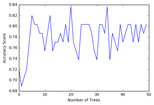
The confusion matrix and accuracy score are similar to that of my previous post (remember, a decision tree is pseudo-randomly created, so results will be similar, but not identical, when run with the same dataset). Examining the relative importance of each attribute is interesting here. As expected, income per person is the most highly correlated with internet use rate, at 54% of the model’s predictive capability. Employment rate (15%) and female employment rate (11%) are less correlated, again, as expected. But polity score, at 20% of the model’s predictive capability, stood out to me because none of the previous models I’ve examined with this dataset have had polity score even near the same level of importance as employment rates. Interesting. Finally, the graph shows that as the number of trees in the forest grows, the accuracy of the model does as well, but only up to about 20 trees. After that, the accuracy stops increasing and instead fluctuates with the random permutations of the subsets of data that were used to create the trees.

[ramu3218]

Running a Classification Tree

Machine Learning for Data Analysis

Running a Classification Tree

For the next few posts, I’ll be exploring machine learning techniques to help analyze the GapMinder data. To begin, I’ll create a classification tree to explore the relationship between my response variable, internet user rate, and my explanatory variables, income per person, employment rate, female employment rate, and polity score. The technique requires a binary, categorical response variable, so for the purpose of this demonstration I have binned internet use rate into two categories, High usage and Low usage, split by the median data point.

Load the data and convert the variables to numeric

In [1]:''' Code for Peer-graded Assignments: Running a Classification Tree Course: Data Management and Visualization Specialization: Data Analysis and Interpretation ''' import pandas as pd from sklearn.cross_validation import train_test_split from sklearn.tree import DecisionTreeClassifier import sklearn.metrics data = pd.read_csv('c:/users/greg/desktop/gapminder.csv', low_memory=False) data['internetuserate'] = pd.to_numeric(data['internetuserate'], errors='coerce') data['incomeperperson'] = pd.to_numeric(data['incomeperperson'], errors='coerce') data['employrate'] = pd.to_numeric(data['employrate'], errors='coerce') data['femaleemployrate'] = pd.to_numeric(data['femaleemployrate'], errors='coerce') data['polityscore'] = pd.to_numeric(data['polityscore'], errors='coerce')

Convert the response variable to binary

In [3]:binarydata = data.copy() def internetgrp (row): if row['internetuserate'] < data['internetuserate'].median(): return 0 else: return 1 binarydata['internetuserate'] = binarydata.apply (lambda row: internetgrp (row),axis=1)

Clean the data by discarding NA values

In [4]:binarydata_clean = binarydata.dropna() binarydata_clean.dtypes binarydata_clean.describe()

Out[4]:incomeperpersonfemaleemployrateinternetuseratepolityscoreemployratecount152.000000152.000000152.000000152.000000152.000000mean6706.55697848.0684210.4539473.86184259.212500std9823.59231514.8268570.4995216.24558110.363802min103.77585712.4000000.000000-10.00000034.90000225%560.79715839.5499990.000000-2.00000051.92499950%2225.93101948.5499990.0000007.00000058.90000275%6905.28766256.0500001.0000009.00000065.000000max39972.35276883.3000031.00000010.00000083.199997

Split into training and testing sets

In [7]:predictors = binarydata_clean[['incomeperperson','employrate','femaleemployrate','polityscore']] targets = binarydata_clean.internetuserate pred_train, pred_test, tar_train, tar_test = train_test_split(predictors, targets, test_size=.4) print ('Training sample') print (pred_train.shape) print ('') print ('Testing sample') print (pred_test.shape) print ('') print ('Training sample') print (tar_train.shape) print ('') print ('Testing sample') print (tar_test.shape) Training sample (91, 4) Testing sample (61, 4) Training sample (91,) Testing sample (61,)

Build model on the training data

In [8]:classifier=DecisionTreeClassifier() classifier=classifier.fit(pred_train,tar_train) predictions=classifier.predict(pred_test)

Display the confusion matrix

In [10]:sklearn.metrics.confusion_matrix(tar_test,predictions)

Out[10]:array([[22, 9], [ 8, 22]])

Display the accuracy score

In [11]:sklearn.metrics.accuracy_score(tar_test, predictions)

Out[11]:0.72131147540983609

Display the decision tree

In [13]:from sklearn import tree from io import StringIO from IPython.display import Image out = StringIO() tree.export_graphviz(classifier, out_file=out) import pydotplus graph=pydotplus.graph_from_dot_data(out.getvalue()) Image(graph.create_png())

Out[13]:

The decision tree analysis was performed to test non-linear relationships among the explanatory variables and a single binary, categorical response variable. The training sample has 91 rows of data and 4 explanatory variables; the testing sample has 61 rows of data, and the same 4 explanatory variables. The decision tree results in 27 true negatives and 16 true positives; and 11 false negatives and 7 false positives. The accuracy score is 70.5%, meaning that the model accurately predicted 70.5% of the internet use rates per country.

[ramu3218]

Logistic Regression Model

import numpy

import pandas

import statsmodels.api as sm

import seaborn

import statsmodels.formula.api as smf

# bug fix for display formats to avoid run time errorspandas.set_option('display.float_format', lambda x:'%.2f'%x)nesarc = pandas.read_csv ('nesarc_pds.csv' , low_memory=False)

#Set PANDAS to show all columns in DataFramepandas.set_option('display.max_columns', None)

#Set PANDAS to show all rows in DataFramepandas.set_option('display.max_rows', None) nesarc.columns = map(str.upper , nesarc.columns)

# Change my variables to numeric nesarc['S3BQ1A5'] = pandas.to_numeric(nesarc['S3BQ1A5'], errors='coerce')nesarc['MARP12ABDEP'] = pandas.to_numeric(nesarc['MARP12ABDEP'], errors='coerce') # Cannabis abuse/dependencenesarc['COCP12ABDEP'] = pandas.to_numeric(nesarc['COCP12ABDEP'], errors='coerce') # Cocaine abuse/dependencenesarc['ALCABDEPP12DX'] = pandas.to_numeric(nesarc['ALCABDEPP12DX'], errors='coerce') # Alcohol abuse/dependencenesarc['HERP12ABDEP'] = pandas.to_numeric(nesarc['HERP12ABDEP'], errors='coerce')

# Heroin abuse/dependencenesarc['MAJORDEP12'] = pandas.to_numeric(nesarc['MAJORDEP12'], errors='coerce')

# Major depression # Subset my sample: ages 18-30 sub1=nesarc[(nesarc['AGE']>=18) & (nesarc['AGE']<=30)] ############################################################################### LOGISTIC REGRESSION############################################################################## # Binary cannabis abuse/dependence prior to the last 12 months def CANDEPPR12 (x1): if x1['MARP12ABDEP']==1 or x1['MARP12ABDEP']==2 or x1['MARP12ABDEP']==3: return 1 else: return 0sub1['CANDEPPR12'] = sub1.apply (lambda x1: CANDEPPR12 (x1), axis=1)print (pandas.crosstab(sub1['MARP12ABDEP'], sub1['CANDEPPR12'])) ## Logistic regression with cannabis abuse/dependence (explanatory) - major depression (response) logreg1 = smf.logit(formula = 'MAJORDEP12 ~ CANDEPPR12', data = sub1).fit()print (logreg1.summary())# odds ratiosprint ("Odds Ratios")print (numpy.exp(logreg1.params))

# Odd ratios with 95% confidence intervals params = logreg1.paramsconf = logreg1.conf_int()conf['OR'] = paramsconf.columns = ['Lower CI', 'Upper CI', 'OR']print (numpy.exp(conf))

# Binary cocaine abuse/dependence prior to the last 12 months def COCDEPPR12 (x2): if x2['COCP12ABDEP']==1 or x2['COCP12ABDEP']==2 or x2['COCP12ABDEP']==3: return 1 else: return 0sub1['COCDEPPR12'] = sub1.apply (lambda x2: COCDEPPR12 (x2), axis=1)print (pandas.crosstab(sub1['COCP12ABDEP'], sub1['COCDEPPR12']))

## Logistic regression with cannabis and cocaine abuse/depndence (explanatory) - major depression (response) logreg2 = smf.logit(formula = 'MAJORDEP12 ~ CANDEPPR12 + COCDEPPR12', data = sub1).fit()print (logreg2.summary()) # Odd ratios with 95% confidence intervals params = logreg2.paramsconf = logreg2.conf_int()conf['OR'] = paramsconf.columns = ['Lower CI', 'Upper CI', 'OR']print (numpy.exp(conf))

# Binary alcohol abuse/dependence prior to the last 12 months def ALCDEPPR12 (x2): if x2['ALCABDEPP12DX']==1 or x2['ALCABDEPP12DX']==2 or x2['ALCABDEPP12DX']==3: return 1 else: return 0sub1['ALCDEPPR12'] = sub1.apply (lambda x2: ALCDEPPR12 (x2), axis=1)print (pandas.crosstab(sub1['ALCABDEPP12DX'], sub1['ALCDEPPR12']))

# Binary sedative abuse/dependence prior to the last 12 months def HERDEPPR12 (x3): if x3['HERP12ABDEP']==1 or x3['HERP12ABDEP']==2 or x3['HERP12ABDEP']==3: return 1 else: return 0sub1['HERDEPPR12'] = sub1.apply (lambda x3: HERDEPPR12 (x3), axis=1)print (pandas.crosstab(sub1['HERP12ABDEP'], sub1['HERDEPPR12']))

## Logistic regression with alcohol abuse/depndence (explanatory) - major depression (response) logreg3 = smf.logit(formula = 'MAJORDEP12 ~ HERDEPPR12', data = sub1).fit()print (logreg3.summary()) # Odd ratios with 95% confidence intervals print ("Odds Ratios")params = logreg3.paramsconf = logreg3.conf_int()conf['OR'] = paramsconf.columns = ['Lower CI', 'Upper CI', 'OR']print (numpy.exp(conf))

## Logistic regression with cannabis and alcohol abuse/depndence (explanatory) - major depression (response) logreg4 = smf.logit(formula = 'MAJORDEP12 ~ CANDEPPR12 + ALCDEPPR12 + COCDEPPR12', data = sub1).fit()print (logreg4.summary()) # Odd ratios with 95% confidence intervals print ("Odds Ratios")params = logreg4.paramsconf = logreg4.conf_int()conf['OR'] = paramsconf.columns = ['Lower CI', 'Upper CI', 'OR']print (numpy.exp(conf))

result:

[ramu3218]

MULTIPLE REGRESSION MODEL

import numpy

import pandas

import statsmodels.api as sm

import seaborn

import statsmodels.formula.api as smf

import matplotlib.pyplot as plt

# bug fix for display formats to avoid run time errorspandas.set_option('display.float_format', lambda x:'%.2f'%x)nesarc = pandas.read_csv ('nesarc_pds.csv' , low_memory=False)

#Set PANDAS to show all columns in DataFramepandas.set_option('display.max_columns', None)#Set PANDAS to show all rows in DataFramepandas.set_option('display.max_rows', None) nesarc.columns = map(str.upper , nesarc.columns) # Change my variables to numeric nesarc['IDNUM'] =pandas.to_numeric(nesarc['IDNUM'], errors='coerce')nesarc['S3BQ1A5'] = pandas.to_numeric(nesarc['S3BQ1A5'], errors='coerce')nesarc['MAJORDEP12'] = pandas.to_numeric(nesarc['MAJORDEP12'], errors='coerce') # Major depressionnesarc['AGE'] =pandas.to_numeric(nesarc['AGE'], errors='coerce')nesarc['SEX'] = pandas.to_numeric(nesarc['SEX'], errors='coerce')nesarc['S3BD5Q2E'] = pandas.to_numeric(nesarc['S3BD5Q2E'], errors='coerce') # Cannabis use frequencynesarc['S3BQ4'] = pandas.to_numeric(nesarc['S3BQ4'], errors='coerce') # Quantity of joints per daynesarc['GENAXDX12'] = pandas.to_numeric(nesarc['GENAXDX12'], errors='coerce') # General anxietynesarc['S3BD5Q2F'] = pandas.to_numeric(nesarc['S3BD5Q2F'], errors='coerce') # Age when began using cannabis the mostnesarc['DYSDX12'] = pandas.to_numeric(nesarc['DYSDX12'], errors='coerce')

# Dysthymianesarc['SOCPDX12'] = pandas.to_numeric(nesarc['SOCPDX12'], errors='coerce') # Social phobianesarc['S3BD5Q2GR'] = pandas.to_numeric(nesarc['S3BD5Q2GR'], errors='coerce') # Cannabis use duration (weeks)nesarc['S3CD5Q15C'] = pandas.to_numeric(nesarc['S3CD5Q15C'], errors='coerce') # Cannabis dependencenesarc['S3CD5Q13B'] = pandas.to_numeric(nesarc['S3CD5Q13B'], errors='coerce')

# Cannabis abuse # Current cannabis abuse criterianesarc['S3CD5Q14C9'] = pandas.to_numeric(nesarc['S3CD5Q14C9'], errors='coerce')nesarc['S3CQ14A8'] = pandas.to_numeric(nesarc['S3CQ14A8'], errors='coerce') # Longer period cannabis abuse criterianesarc['S3CD5Q14C3'] = pandas.to_numeric(nesarc['S3CD5Q14C3'], errors='coerce') # Depressed because of cannabis effects wearing offnesarc['S3CD5Q14C6C'] = pandas.to_numeric(nesarc['S3CD5Q14C6C'], errors='coerce') # Sleep difficulties because of cannabis effects wearing offnesarc['S3CD5Q14C6R'] = pandas.to_numeric(nesarc['S3CD5Q14C6R'], errors='coerce')

# Eat more because of cannabis effects wearing offnesarc['S3CD5Q14C6H'] = pandas.to_numeric(nesarc['S3CD5Q14C6H'], errors='coerce') # Feel nervous or anxious because of cannabis effects wearing offnesarc['S3CD5Q14C6I'] = pandas.to_numeric(nesarc['S3CD5Q14C6I'], errors='coerce')

# Fast heart beat because of cannabis effects wearing offnesarc['S3CD5Q14C6D'] = pandas.to_numeric(nesarc['S3CD5Q14C6D'], errors='coerce') # Feel weak or tired because of cannabis effects wearing offnesarc['S3CD5Q14C6B'] = pandas.to_numeric(nesarc['S3CD5Q14C6B'], errors='coerce')

# Withdrawal symptomsnesarc['S3CD5Q14C6U'] = pandas.to_numeric(nesarc['S3CD5Q14C6U'], errors='coerce')

# Subset my sample: Cannabis users, ages 18-30 sub1=nesarc[(nesarc['AGE']>=18) & (nesarc['AGE']<=30) & (nesarc['S3BQ1A5']==1)] ###############

Cannabis abuse/dependence criteria in the last 12 months (response variable) ############### #

Current cannabis abuse/dependence criteria #1 DSM-IV def crit1 (row): if row['S3CD5Q14C9']==1 or row['S3CQ14A8'] == 1 : return 1 elif row['S3CD5Q14C9']==2 and row['S3CQ14A8']==2 : return 0sub1['crit1'] = sub1.apply (lambda row: crit1 (row),axis=1) # Current 6 cannabis abuse/dependence sub-symptoms criteria #2 DSM-IV # Recode for summing (from 1,2 to 0,1)recode1 = {1: 1, 2: 0}sub1['S3CD5Q14C6C']=sub1['S3CD5Q14C6C'].replace(9, numpy.nan)sub1['S3CD5Q14C6C']= sub1['S3CD5Q14C6C'].map(recode1)sub1['S3CD5Q14C6R']=sub1['S3CD5Q14C6R'].replace(9, numpy.nan)sub1['S3CD5Q14C6R']= sub1['S3CD5Q14C6R'].map(recode1)sub1['S3CD5Q14C6H']=sub1['S3CD5Q14C6H'].replace(9, numpy.nan)sub1['S3CD5Q14C6H']= sub1['S3CD5Q14C6H'].map(recode1)sub1['S3CD5Q14C6I']=sub1['S3CD5Q14C6I'].replace(9, numpy.nan)sub1['S3CD5Q14C6I']= sub1['S3CD5Q14C6I'].map(recode1)sub1['S3CD5Q14C6D']=sub1['S3CD5Q14C6D'].replace(9, numpy.nan)sub1['S3CD5Q14C6D']= sub1['S3CD5Q14C6D'].map(recode1)sub1['S3CD5Q14C6B']=sub1['S3CD5Q14C6B'].replace(9, numpy.nan)sub1['S3CD5Q14C6B']= sub1['S3CD5Q14C6B'].map(recode1)

# Sum symptomssub1['CWITHDR_COUNT'] = numpy.nansum([sub1['S3CD5Q14C6C'], sub1['S3CD5Q14C6R'], sub1['S3CD5Q14C6H'], sub1['S3CD5Q14C6I'], sub1['S3CD5Q14C6D'], sub1['S3CD5Q14C6B']], axis=0) # Sum code checkchksum=sub1[['IDNUM','S3CD5Q14C6C', 'S3CD5Q14C6R', 'S3CD5Q14C6H', 'S3CD5Q14C6I', 'S3CD5Q14C6D', 'S3CD5Q14C6B', 'CWITHDR_COUNT']]chksum.head(n=50)

# Withdrawal symptoms in the last 12 months (yes/no)def crit2 (row): if row['CWITHDR_COUNT']>=3 or row['S3CD5Q14C6U']==1: return 1 elif row['CWITHDR_COUNT']<3 and row['S3CD5Q14C6U']!=1: return 0sub1['crit2'] = sub1.apply (lambda row: crit2 (row),axis=1) # Longer period cannabis abuse/dependence criteria #3 DSM-IV sub1['S3CD5Q14C3']=sub1['S3CD5Q14C3'].replace(9, numpy.nan)sub1['S3CD5Q14C3']= sub1['S3CD5Q14C3'].map(recode1)

# Current cannabis use cut down criteria #4 DSM-IV sub1['S3CD5Q14C2'] = pandas.to_numeric(sub1['S3CD5Q14C2'], errors='coerce') # Without successsub1['S3CD5Q14C1'] = pandas.to_numeric(sub1['S3CD5Q14C1'], errors='coerce') # More than oncedef crit4 (row): if row['S3CD5Q14C2']==1 or row['S3CD5Q14C1'] == 1 : return 1 elif row['S3CD5Q14C2']==2 and row['S3CD5Q14C1']==2 : return 0sub1['crit4'] = sub1.apply (lambda row: crit4 (row),axis=1)chk1e = sub1['crit4'].value_counts(sort=False, dropna=False)

# Current reduce of important/pleasurable activities criteria #5 DSM-IV sub1['S3CD5Q14C10'] = pandas.to_numeric(sub1['S3CD5Q14C10'], errors='coerce')sub1['S3CD5Q14C11'] = pandas.to_numeric(sub1['S3CD5Q14C11'], errors='coerce')def crit5 (row): if row['S3CD5Q14C10']==1 or row['S3CD5Q14C11'] == 1 : return 1 elif row['S3CD5Q14C10']==2 and row['S3CD5Q14C11']==2 : return 0sub1['crit5'] = sub1.apply (lambda row: crit5 (row),axis=1)chk1g = sub1['crit5'].value_counts(sort=False, dropna=False) # Current cannbis use continuation despite knowledge of physical or psychological problem criteria

#6 DSM-IV sub1['S3CD5Q14C13'] = pandas.to_numeric(sub1['S3CD5Q14C13'], errors='coerce')sub1['S3CD5Q14C12'] = pandas.to_numeric(sub1['S3CD5Q14C12'], errors='coerce')def crit6 (row): if row['S3CD5Q14C13']==1 or row['S3CD5Q14C12'] == 1 : return 1 elif row['S3CD5Q14C13']==2 and row['S3CD5Q14C12']==2 : return 0sub1['crit6'] = sub1.apply (lambda row: crit6 (row),axis=1)chk1h = sub1['crit6'].value_counts(sort=False, dropna=False)

# Cannabis abuse/dependence symptoms sum sub1['CanDepSymptoms'] = numpy.nansum([sub1['crit1'], sub1['crit2'], sub1['S3CD5Q14C3'], sub1['crit4'], sub1['crit5'], sub1['crit6']], axis=0 )chk2 = sub1['CanDepSymptoms'].value_counts(sort=False, dropna=False) ############################################################################### MULTIPLE REGRESSION & CONFIDENCE INTERVALS

############################################################################## sub2 = sub1[['S3BQ4', 'S3BD5Q2F', 'DYSDX12', 'MAJORDEP12', 'CanDepSymptoms', 'SOCPDX12', 'GENAXDX12', 'S3BD5Q2GR']].dropna()

# Centre the quantity of joints smoked per day and age when they began using cannabis, quantitative variablessub1['numberjosmoked_c'] = (sub1['S3BQ4'] - sub1['S3BQ4'].mean())sub1['agebeganuse_c'] = (sub1['S3BD5Q2F'] - sub1['S3BD5Q2F'].mean())sub1['canuseduration_c'] = (sub1['S3BD5Q2GR'] - sub1['S3BD5Q2GR'].mean()) # Linear regression analysis print('OLS regression model for the association between major depression diagnosis and cannabis depndence symptoms')reg1 = smf.ols('CanDepSymptoms ~ MAJORDEP12', data=sub1).fit()print (reg1.summary()) print('OLS regression model for the association of majord depression diagnosis and smoking quantity with cannabis dependence symptoms')reg2 = smf.ols('CanDepSymptoms ~ MAJORDEP12 + DYSDX12', data=sub1).fit()print (reg2.summary()) reg3 = smf.ols('CanDepSymptoms ~ MAJORDEP12 + agebeganuse_c + numberjosmoked_c + canuseduration_c + GENAXDX12 + DYSDX12 + SOCPDX12', data=sub1).fit()print (reg3.summary())

##################################################################################### POLYNOMIAL REGRESSION

#################################################################################### #

First order (linear) scatterplotscat1 = seaborn.regplot(x="S3BQ4", y="CanDepSymptoms", scatter=True, data=sub1)plt.ylim(0, 6)plt.xlabel('Quantity of joints')plt.ylabel('Cannabis dependence symptoms') # Fit second order polynomialscat1 = seaborn.regplot(x="S3BQ4", y="CanDepSymptoms", scatter=True, order=2, data=sub1)plt.ylim(0, 6)plt.xlabel('Quantity of joints')plt.ylabel('Cannabis dependence symptoms') # Linear regression analysisreg4 = smf.ols('CanDepSymptoms ~ numberjosmoked_c', data=sub1).fit()print (reg4.summary()) reg5 = smf.ols('CanDepSymptoms ~ numberjosmoked_c + I(numberjosmoked_c**2)',

data=sub1).fit()print (reg5.summary()) ##################################################################################### EVALUATING MODEL FIT

####################################################################################

recode1 = {1: 10, 2: 9, 3: 8, 4: 7, 5: 6, 6: 5, 7: 4, 8: 3, 9: 2, 10: 1} # Dictionary with details of frequency variable reverse-recodesub1['CUFREQ'] = sub1['S3BD5Q2E'].map(recode1) # Change variable name from S3BD5Q2E to CUFREQ sub1['CUFREQ_c'] = (sub1['CUFREQ'] - sub1['CUFREQ'].mean()) # Adding frequency of cannabis usereg6 = smf.ols('CanDepSymptoms ~ numberjosmoked_c + I(numberjosmoked_c**2) + CUFREQ_c', data=sub1).fit()print (reg6.summary()) # Q-Q plot for normalityfig1=sm.qqplot(reg6.resid, line='r')print (fig1)

# Simple plot of residualsstdres=pandas.DataFrame(reg6.resid_pearson)fig2=plt.plot(stdres, 'o', ls='None')l = plt.axhline(y=0, color='r')plt.ylabel('Standardized Residual')plt.xlabel('Observation Number') # Additional regression diagnostic plotsfig3 = plt.figure(figsize=(12,8))fig3 = sm.graphics.plot_regress_exog(reg6, "CUFREQ_c", fig=fig3) # leverage plotfig4 = plt.figure(figsize=(36,24))fig4=sm.graphics.influence_plot(reg6, size=2)print(fig4)

OUTPUT:

[ramu3218]

BASIC REGRESSION MODEL

import numpy

import pandas

import statsmodels.api as sm

import seaborn

import statsmodels.formula.api as smf

import matplotlib.pyplot as plt

# bug fix for display formats to avoid run time errorspandas.set_option('display.float_format', lambda x:'%.2f'%x) nesarc = pandas.read_csv ('nesarc_pds.csv' , low_memory=False) #Set PANDAS to show all columns in DataFramepandas.set_option('display.max_columns', None)#Set PANDAS to show all rows in DataFramepandas.set_option('display.max_rows', None) nesarc.columns = map(str.upper , nesarc.columns) # Change my variables to numeric nesarc['IDNUM'] =pandas.to_numeric(nesarc['IDNUM'], errors='coerce')nesarc['S3BQ1A5'] = pandas.to_numeric(nesarc['S3BQ1A5'], errors='coerce')nesarc['MAJORDEP12'] = pandas.to_numeric(nesarc['MAJORDEP12'], errors='coerce')nesarc['AGE'] =pandas.to_numeric(nesarc['AGE'], errors='coerce')nesarc['SEX'] = pandas.to_numeric(nesarc['SEX'], errors='coerce')nesarc['S3BD5Q2E'] = pandas.to_numeric(nesarc['S3BD5Q2E'], errors='coerce') # Current cannabis abuse criterianesarc['S3CD5Q14C9'] = pandas.to_numeric(nesarc['S3CD5Q14C9'], errors='coerce')nesarc['S3CQ14A8'] = pandas.to_numeric(nesarc['S3CQ14A8'], errors='coerce') # Longer period cannabis abuse criterianesarc['S3CD5Q14C3'] = pandas.to_numeric(nesarc['S3CD5Q14C3'], errors='coerce') # Depressed because of cannabis effects wearing offnesarc['S3CD5Q14C6C'] = pandas.to_numeric(nesarc['S3CD5Q14C6C'], errors='coerce') # Sleep difficulties because of cannabis effects wearing offnesarc['S3CD5Q14C6R'] = pandas.to_numeric(nesarc['S3CD5Q14C6R'], errors='coerce') # Eat more because of cannabis effects wearing offnesarc['S3CD5Q14C6H'] = pandas.to_numeric(nesarc['S3CD5Q14C6H'], errors='coerce') # Feel nervous or anxious because of cannabis effects wearing offnesarc['S3CD5Q14C6I'] = pandas.to_numeric(nesarc['S3CD5Q14C6I'], errors='coerce') # Fast heart beat because of cannabis effects wearing offnesarc['S3CD5Q14C6D'] = pandas.to_numeric(nesarc['S3CD5Q14C6D'], errors='coerce') # Feel weak or tired because of cannabis effects wearing offnesarc['S3CD5Q14C6B'] = pandas.to_numeric(nesarc['S3CD5Q14C6B'], errors='coerce') # Withdrawal symptomsnesarc['S3CD5Q14C6U'] = pandas.to_numeric(nesarc['S3CD5Q14C6U'], errors='coerce') # Subset my sample: Cannabis users, ages 18-30 sub1=nesarc[(nesarc['AGE']>=18) & (nesarc['AGE']<=30) & (nesarc['S3BQ1A5']==1)] (pandas.crosstab(sub1['S3CD5Q14C9'], sub1['S3CQ14A8'])) c1 = sub1['S3CD5Q14C6U'].value_counts(sort=False, dropna=False)print (c1) # Current 6 cannabis abuse/dependence sub-symptoms criteria #2 DSM-IV # Recode for summing (from 1,2 to 0,1)recode1 = {1: 1, 2: 0}sub1['S3CD5Q14C6C']=sub1['S3CD5Q14C6C'].replace(9, numpy.nan)sub1['S3CD5Q14C6C']= sub1['S3CD5Q14C6C'].map(recode1)sub1['S3CD5Q14C6R']=sub1['S3CD5Q14C6R'].replace(9, numpy.nan)sub1['S3CD5Q14C6R']= sub1['S3CD5Q14C6R'].map(recode1)sub1['S3CD5Q14C6H']=sub1['S3CD5Q14C6H'].replace(9, numpy.nan)sub1['S3CD5Q14C6H']= sub1['S3CD5Q14C6H'].map(recode1)sub1['S3CD5Q14C6I']=sub1['S3CD5Q14C6I'].replace(9, numpy.nan)sub1['S3CD5Q14C6I']= sub1['S3CD5Q14C6I'].map(recode1)sub1['S3CD5Q14C6D']=sub1['S3CD5Q14C6D'].replace(9, numpy.nan)sub1['S3CD5Q14C6D']= sub1['S3CD5Q14C6D'].map(recode1)sub1['S3CD5Q14C6B']=sub1['S3CD5Q14C6B'].replace(9, numpy.nan)sub1['S3CD5Q14C6B']= sub1['S3CD5Q14C6B'].map(recode1) # Check recodechk1c = sub1['S3CD5Q14C6U'].value_counts(sort=False, dropna=False)print (chk1c) # Sum symptomssub1['CWITHDR_COUNT'] = numpy.nansum([sub1['S3CD5Q14C6C'], sub1['S3CD5Q14C6R'], sub1['S3CD5Q14C6H'], sub1['S3CD5Q14C6I'], sub1['S3CD5Q14C6D'], sub1['S3CD5Q14C6B']], axis=0) # Sum code checkchksum=sub1[['IDNUM','S3CD5Q14C6C', 'S3CD5Q14C6R', 'S3CD5Q14C6H', 'S3CD5Q14C6I', 'S3CD5Q14C6D', 'S3CD5Q14C6B', 'CWITHDR_COUNT']]chksum.head(n=50) chk1d = sub1['CWITHDR_COUNT'].value_counts(sort=False, dropna=False)print (chk1d)

# Withdrawal symptoms in the last 12 months (yes/no)def crit2 (row): if row['CWITHDR_COUNT']>=3 or row['S3CD5Q14C6U']==1: return 1 elif row['CWITHDR_COUNT']<3 and row['S3CD5Q14C6U']!=1: return 0sub1['crit2'] = sub1.apply (lambda row: crit2 (row),axis=1)print (pandas.crosstab(sub1['CWITHDR_COUNT'], sub1['crit2'])) # Longer period cannabis abuse/dependence criteria #3 DSM-IV sub1['S3CD5Q14C3']=sub1['S3CD5Q14C3'].replace(9, numpy.nan)sub1['S3CD5Q14C3']= sub1['S3CD5Q14C3'].map(recode1) chk1d = sub1['S3CD5Q14C3'].value_counts(sort=False, dropna=False)print (chk1d) # Current cannabis use cut down criteria #4 DSM-IV sub1['S3CD5Q14C2'] = pandas.to_numeric(sub1['S3CD5Q14C2'], errors='coerce') # Without successsub1['S3CD5Q14C1'] = pandas.to_numeric(sub1['S3CD5Q14C1'], errors='coerce') # More than oncedef crit4 (row): if row['S3CD5Q14C2']==1 or row['S3CD5Q14C1'] == 1 : return 1 elif row['S3CD5Q14C2']==2 and row['S3CD5Q14C1']==2 : return 0sub1['crit4'] = sub1.apply (lambda row: crit4 (row),axis=1)chk1e = sub1['crit4'].value_counts(sort=False, dropna=False)print (chk1e) # Current reduce of important/pleasurable activities criteria

#5 DSM-IV sub1['S3CD5Q14C10'] = pandas.to_numeric(sub1['S3CD5Q14C10'], errors='coerce')sub1['S3CD5Q14C11'] = pandas.to_numeric(sub1['S3CD5Q14C11'], errors='coerce')def crit5 (row): if row['S3CD5Q14C10']==1 or row['S3CD5Q14C11'] == 1 : return 1 elif row['S3CD5Q14C10']==2 and row['S3CD5Q14C11']==2 : return 0sub1['crit5'] = sub1.apply (lambda row: crit5 (row),axis=1)chk1g = sub1['crit5'].value_counts(sort=False, dropna=False)print (chk1g) # Current cannbis use continuation despite knowledge of physical or psychological problem criteria #6 DSM-IV sub1['S3CD5Q14C13'] = pandas.to_numeric(sub1['S3CD5Q14C13'], errors='coerce')sub1['S3CD5Q14C12'] = pandas.to_numeric(sub1['S3CD5Q14C12'], errors='coerce')def crit6 (row): if row['S3CD5Q14C13']==1 or row['S3CD5Q14C12'] == 1 : return 1 elif row['S3CD5Q14C13']==2 and row['S3CD5Q14C12']==2 : return 0sub1['crit6'] = sub1.apply (lambda row: crit6 (row),axis=1)chk1h = sub1['crit6'].value_counts(sort=False, dropna=False)print (chk1h) # Cannabis abuse/dependence symptoms sum sub1['CanDepSymptoms'] = numpy.nansum([sub1['crit1'], sub1['crit2'], sub1['S3CD5Q14C3'], sub1['crit4'], sub1['crit5'], sub1['crit6']], axis=0 )

chk2 = sub1['CanDepSymptoms'].value_counts(sort=False, dropna=False)

print (chk2) c1 = sub1["MAJORDEP12"].value_counts(sort=False, dropna=False)print(c1)c2 = sub1["AGE"].value_counts(sort=False, dropna=False)print(c2)

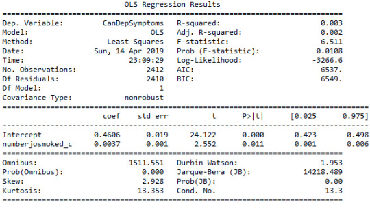
############### Major depression diagnosis in the last 12 months (explanatory variable) ############### # Major depression diagnosis print('OLS regression model for the association between major depression diagnosis and cannabis depndence symptoms')reg1 = smf.ols('CanDepSymptoms ~ MAJORDEP12', data=sub1).fit()print (reg1.summary()) # Listwise deletion for calculating means for regression model observations sub1 = sub1[['CanDepSymptoms', 'MAJORDEP12']].dropna() # Group means & sd print ("Mean")ds1 = sub1.groupby('MAJORDEP12').mean()print (ds1)print ("Standard deviation")ds2 = sub1.groupby('MAJORDEP12').std()print (ds2) # Bivariate bar graph print('Bivariate bar graph for major depression diagnosis and cannabis depndence symptoms')

seaborn.factorplot(x="MAJORDEP12", y="CanDepSymptoms", data=sub1, kind="bar", ci=None)plt.xlabel('Major Depression Diagnosis')plt.ylabel('Mean Number of Cannabis Dependence Symptoms')

[ramu3218]

THE GAPMINDER

Sample

I am using the GapMinder dataset to investigate the relationship between internet usage in a country and that country’s GDP, overall employment rate, female employment rate, and its “polity score”, which is a measure of a country’s democratic and free nature. The sample contains data on a country-level for 215 regions (the 192 U.N. countries, with Serbia and Montenegro aggregated into one, as well as 24 other non-country regions, such as Monaco for instance). The study population is these 215 countries and regions and my sample data is the same; ie, the population is small enough that no sample is necessary to make the data collecting and processing more manageable.

Procedure

The data has been collected by the non-profit venture GapMinder from a handful of sources, including the Institute for Health Metrics and Evaluation, the US Census Bureau’s International Database, the United Nations Statistics Division, and the World Bank. In the case of each data collection organization, data was collected from detailed surveys of the country’s population (such as in a national census) and based mainly upon 2010 data. Employment rate data comes from 2007 and polity score from 2009. Polity score is calculated by subtracting the autocracy score from the democracy score from the Polity IV project’s research. GapMinder’s goal in collecting this data is to help world leaders and their citizens to better understand the forces shaping the geopolitical landscape around the globe.

Measures

My response variable is the internet use rate and my explanatory variables are income per person, employment rate, female employment rate, and polity score. Internet use rate, employment rate, and female employment rate are scaled as percentages of the country’s population. Income per person is simply Gross Domestic Product per capita (the country’s total, country-wide income divided by the population). Polity score is a single measure applied to the whole country. The internet use rate of a country was collected by the World Bank in their World Development Indicators. Income per person is simply the 2010 Gross Domestic Product per capita in constant 2000 USD. The inflation, but not the differences in the cost of living between countries, has been taken into account (this can lead to the seemingly odd case of a having negative income per person, when that country already has very low income relative to the United States plus high inflation, relative to the United States). Both employment rate and female employment rate have been provided by the International Labour Organization. Finally, the polity score has been calculated by the Polity IV project.

I have gone through the data and removed entries where data is missing, when necessary, and sometimes have aggregated data into bins, for histograms, for instance, but otherwise have not modified the data in any way. Deeper data management was unnecessary for the analysis.

[ramu3218]

Testing a potential Moderator

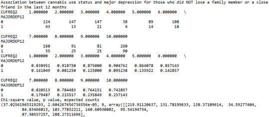
import pandasimport numpy import seabornimport scipyimport matplotlib.pyplot as plt nesarc = pandas.read_csv ('nesarc_pds.csv', low_memory=False) # Set PANDAS to show all columns in DataFramepandas.set_option('display.max_columns' , None) # Set PANDAS to show all rows in DataFramepandas.set_option('display.max_rows' , None) nesarc.columns = map(str.upper , nesarc.columns) pandas.set_option('display.float_format' , lambda x:'%f'%x) # Change my variables to numeric nesarc['AGE'] = nesarc['AGE'].convert_objects(convert_numeric=True)nesarc['MAJORDEP12'] = nesarc['MAJORDEP12'].convert_objects(convert_numeric=True)nesarc['S1Q231'] = nesarc['S1Q231'].convert_objects(convert_numeric=True)nesarc['S3BQ1A5'] = nesarc['S3BQ1A5'].convert_objects(convert_numeric=True)nesarc['S3BD5Q2E'] = nesarc['S3BD5Q2E'].convert_objects(convert_numeric=True) # Subset my sample subset1 = nesarc[(nesarc['AGE']>=18) & (nesarc['AGE']<=30) & nesarc['S3BQ1A5']==1] # Ages 18-30, cannabis userssubsetc1 = subset1.copy() # Setting missing data subsetc1['S1Q231']=subsetc1['S1Q231'].replace(9, numpy.nan)subsetc1['S3BQ1A5']=subsetc1['S3BQ1A5'].replace(9, numpy.nan)subsetc1['S3BD5Q2E']=subsetc1['S3BD5Q2E'].replace(99, numpy.nan)subsetc1['S3BD5Q2E']=subsetc1['S3BD5Q2E'].replace('BL', numpy.nan) recode1 = {1: 9, 2: 8, 3: 7, 4: 6, 5: 5, 6: 4, 7: 3, 8: 2, 9: 1} # Frequency of cannabis use variable reverse-recodesubsetc1['CUFREQ'] = subsetc1['S3BD5Q2E'].map(recode1) # Change the variable name from S3BD5Q2E to CUFREQ subsetc1['CUFREQ'] = subsetc1['CUFREQ'].astype('category') # Raname graph labels for better interpetation subsetc1['CUFREQ'] = subsetc1['CUFREQ'].cat.rename_categories(["2 times/year","3-6 times/year","7-11 times/year","Once a month","2-3 times/month","1-2 times/week","3-4 times/week","Nearly every day","Every day"]) ## Contingency table of observed counts of major depression diagnosis (response variable) within frequency of cannabis use groups (explanatory variable), in ages 18-30 contab1 = pandas.crosstab(subsetc1['MAJORDEP12'], subsetc1['CUFREQ'])print (contab1) # Column percentages colsum=contab1.sum(axis=0)colpcontab=contab1/colsumprint(colpcontab) # Chi-square calculations for major depression within frequency of cannabis use groups print ('Chi-square value, p value, expected counts, for major depression within cannabis use status')chsq1= scipy.stats.chi2_contingency(contab1)print (chsq1) # Bivariate bar graph for major depression percentages with each cannabis smoking frequency group plt.figure(figsize=(12,4)) # Change plot sizeax1 = seaborn.factorplot(x="CUFREQ", y="MAJORDEP12", data=subsetc1, kind="bar", ci=None)ax1.set_xticklabels(rotation=40, ha="right") # X-axis labels rotationplt.xlabel('Frequency of cannabis use')plt.ylabel('Proportion of Major Depression')plt.show() recode2 = {1: 10, 2: 9, 3: 8, 4: 7, 5: 6, 6: 5, 7: 4, 8: 3, 9: 2, 10: 1} # Frequency of cannabis use variable reverse-recodesubsetc1['CUFREQ2'] = subsetc1['S3BD5Q2E'].map(recode2) # Change the variable name from S3BD5Q2E to CUFREQ2 sub1=subsetc1[(subsetc1['S1Q231']== 1)]sub2=subsetc1[(subsetc1['S1Q231']== 2)] print ('Association between cannabis use status and major depression for those who lost a family member or a close friend in the last 12 months')contab2=pandas.crosstab(sub1['MAJORDEP12'], sub1['CUFREQ2'])print (contab2) # Column percentages colsum2=contab2.sum(axis=0)colpcontab2=contab2/colsum2print(colpcontab2) # Chi-square print ('Chi-square value, p value, expected counts')

chsq2= scipy.stats.chi2_contingency(contab2)print (chsq2) # Line graph for major depression percentages within each frequency group, for those who lost a family member or a close friend plt.figure(figsize=(12,4)) # Change plot sizeax2 = seaborn.factorplot(x="CUFREQ", y="MAJORDEP12", data=sub1, kind="point", ci=None)ax2.set_xticklabels(rotation=40, ha="right") # X-axis labels rotationplt.xlabel('Frequency of cannabis use')plt.ylabel('Proportion of Major Depression')

plt.title('Association between cannabis use status and major depression for those who lost a family member or a close friend in the last 12 months')plt.show()

output:

[ramu3218]

Generating correlaton coefficient Assignment

import pandasimport numpyimport seabornimport scipyimport matplotlib.pyplot as plt nesarc = pandas.read_csv ('nesarc_pds.csv' , low_memory=False) #Set PANDAS to show all columns in DataFramepandas.set_option('display.max_columns', None)#Set PANDAS to show all rows in DataFramepandas.set_option('display.max_rows', None) nesarc.columns = map(str.upper , nesarc.columns) pandas.set_option('display.float_format' , lambda x:'%f'%x) # Change my variables to numeric nesarc['AGE'] = pandas.to_numeric(nesarc['AGE'], errors='coerce')nesarc['S3BQ4'] = pandas.to_numeric(nesarc['S3BQ4'], errors='coerce')nesarc['S4AQ6A'] = pandas.to_numeric(nesarc['S4AQ6A'], errors='coerce')nesarc['S3BD5Q2F'] = pandas.to_numeric(nesarc['S3BD5Q2F'], errors='coerce')nesarc['S9Q6A'] = pandas.to_numeric(nesarc['S9Q6A'], errors='coerce')nesarc['S4AQ7'] = pandas.to_numeric(nesarc['S4AQ7'], errors='coerce')nesarc['S3BQ1A5'] = pandas.to_numeric(nesarc['S3BQ1A5'], errors='coerce') # Subset my sample subset1 = nesarc[(nesarc['S3BQ1A5']==1)] # Cannabis userssubsetc1 = subset1.copy() # Setting missing data subsetc1['S3BQ1A5']=subsetc1['S3BQ1A5'].replace(9, numpy.nan)subsetc1['S3BD5Q2F']=subsetc1['S3BD5Q2F'].replace('BL', numpy.nan)subsetc1['S3BD5Q2F']=subsetc1['S3BD5Q2F'].replace(99, numpy.nan)subsetc1['S4AQ6A']=subsetc1['S4AQ6A'].replace('BL', numpy.nan)subsetc1['S4AQ6A']=subsetc1['S4AQ6A'].replace(99, numpy.nan)subsetc1['S9Q6A']=subsetc1['S9Q6A'].replace('BL', numpy.nan)subsetc1['S9Q6A']=subsetc1['S9Q6A'].replace(99, numpy.nan) # Scatterplot for the age when began using cannabis the most and the age of first episode of major depression plt.figure(figsize=(12,4)) # Change plot size scat1 = seaborn.regplot(x="S3BD5Q2F", y="S4AQ6A", fit_reg=True, data=subset1)plt.xlabel('Age when began using cannabis the most')plt.ylabel('Age when expirenced the first episode of major depression')plt.title('Scatterplot for the age when began using cannabis the most and the age of first the episode of major depression')plt.show() data_clean=subset1.dropna() # Pearson correlation coefficient for the age when began using cannabis the most and the age of first the episode of major depression print ('Association between the age when began using cannabis the most and the age of the first episode of major depression')print (scipy.stats.pearsonr(data_clean['S3BD5Q2F'], data_clean['S4AQ6A'])) # Scatterplot for the age when began using cannabis the most and the age of the first episode of general anxiety plt.figure(figsize=(12,4)) # Change plot size scat2 = seaborn.regplot(x="S3BD5Q2F", y="S9Q6A", fit_reg=True, data=subset1)plt.xlabel('Age when began using cannabis the most')plt.ylabel('Age when expirenced the first episode of general anxiety')plt.title('Scatterplot for the age when began using cannabis the most and the age of the first episode of general anxiety')plt.show() # Pearson correlation coefficient for the age when began using cannabis the most and the age of the first episode of general anxiety print ('Association between the age when began using cannabis the most and the age of first the episode of general anxiety')print (scipy.stats.pearsonr(data_clean['S3BD5Q2F'], data_clean['S9Q6A']))

Output

The scatterplot presented above, illustrates the correlation between the age when individuals began using cannabis the most (quantitative explanatory variable) and the age when they experienced the first episode of depression (quantitative response variable). The direction of the relationship is positive (increasing), which means that an increase in the age of cannabis use is associated with an increase in the age of the first depression episode. In addition, since the points are scattered about a line, the relationship is linear. Regarding the strength of the relationship, from the pearson correlation test we can see that the correlation coefficient is equal to 0.23, which indicates a weak linear relationship between the two quantitative variables. The associated p-value is equal to 2.27e-09 (p-value is written in scientific notation) and the fact that its is very small means that the relationship is statistically significant. As a result, the association between the age when began using cannabis the most and the age of the first depression episode is moderately weak, but it is highly unlikely that a relationship of this magnitude would be due to chance alone. Finally, by squaring the r, we can find the fraction of the variability of one variable that can be predicted by the other, which is fairly low at 0.05.

For the association between the age when individuals began using cannabis the most (quantitative explanatory variable) and the age when they experienced the first episode of anxiety (quantitative response variable), the scatterplot psented above shows a positive linear relationship. Regarding the strength of the relationship, the pearson correlation test indicates that the correlation coefficient is equal to 0.14, which is interpreted to a fairly weak linear relationship between the two quantitative variables. The associated p-value is equal to 0.0001, which means that the relationship is statistically significant. Therefore, the association between the age when began using cannabis the most and the age of the first anxiety episode is weak, but it is highly unlikely that a relationship of this magnitude would be due to chance alone. Finally, by squaring the r, we can find the fraction of the variability of one variable that can be predicted by the other, which is very low at 0.01.

[ramu3218]

chi-square test of independence

import pandas as

pd import seaborn as sns

import scipy.stats

data = pd.read_csv('c:/users/greg/desktop/gapminder.csv', low_memory=False) Set the variables to numeric

data['internetuserate'] = pd.to_numeric(data['internetuserate'], errors='coerce') data['polityscore'] = pd.to_numeric(data['polityscore'], errors='coerce')

sub1 = data.copy() Create dataframe with NAs dropped and internetuserate binned to be 'Low' and 'High,' and polityscore is binned to be 'Low,' 'Mid,' and 'High.'

sub3 = sub1[['internetuserate', 'polityscore']].dropna() sub3['polityscore_binned'] = pd.cut(sub3.polityscore, 3, labels=['Low', 'Mid', 'High']) sub3['internetuserate_binned'] = pd.cut(sub3.internetuserate, 2, labels=['Low', 'High'])

sub4 = sub3.copy() Perform Chi-Square test for categorical to categorical variable comparison Contingency table of observed counts

ct2=pd.crosstab(sub4['internetuserate_binned'], sub4['COMP-Low-v-Mid']) ct2 COMP-Low-v-Mid Low Mid internetuserate_binned Low 23 27 High 5 1 Column percentages

colsum=ct2.sum(axis=0) colpct=ct2/colsum colpct COMP-Low-v-Mid Low Mid internetuserate_binned Low 0.821429 0.964286 High 0.178571 0.035714 Chi-square value, p-value, expected counts

cs2= scipy.stats.chi2_contingency(ct2) cs2 (1.6799999999999999, 0.1949244525136572, 1, array([[ 25., 25.], [ 3., 3.]])) Compare Low Polity Score with High Polity Score recode2 = {'Low': 'Low', 'High': 'High'}

cs4= scipy.stats.chi2_contingency(ct4) cs4 (10.336242989794879, 0.00130443250866551, 1, array([[ 69.37795276, 19.62204724], [ 29.62204724, 8.37795276]])) An interesting result of the data is that countries with the lowest internet use rates fall in the mid-range of polity scores (96% of low internet use countries have a polity score between -3 and +3). I attribute this to the fact that countries with both very high and very low polity scores have to have significantly developed governments and infrastructure systems in place in order to control the citizens of the country with either the rule of law (countries with high polity scores) or the rule of a strong-arm dictator (countries with low polity scores). Both of these types of countries need infrastructure, and therefore internet, to survive. However, countries with middle polity scores are more tribal and less likely to have infrastructure such as internet. An X2 of 14.1 and p-value of 0.00086 means these findings are significant.

Post hoc comparisons of internet rates by polity score show that internet use rates were statistically different for the Mid to High polity score comparison, with a p-value of 0.00130 (< 0.003 of the Bonferroni Adjustment). Conversely, the Low to Mid and Low to High comparisons did not exceed the Bonferroni Adjustment, with p-values of 0.195 and 00872, respectively

Blaze

[ramu3218]

Analysis of Variance Below is the code to make the ANOVA technique:

First I have imported the libraries and management the data like in the other assignments presented until here.

import pandas import numpy import statistics import statsmodels.formula.api as smf import statsmodels.stats.multicomp as multi

Import the data set to memory

data = pandas.read_csv("separatedData.csv", low_memory = False)

Change data type among variables to numeric

data["breastCancer100th"] = data["breastCancer100th"].convert_objects(convert_numeric=True) data["meanSugarPerson"] = data["meanSugarPerson"].convert_objects(convert_numeric=True)

Create a subData with only the variables breastCancer100th, meanSugarPerson, meanFoodPerson, meanCholesterol

sub1=data[['breastCancer100th', 'meanSugarPerson']]

Create the conditions to a new variable named sugar_consumption that will categorize the meanSugarPerson answers

def sugar_consumption (row): if 0 < row['meanSugarPerson'] <= 30 : return 0 # Desirable between 0 and 30 g. if 30 < row['meanSugarPerson'] <= 60 : return 1 # Raised between 30 and 60 g. if 60 < row['meanSugarPerson'] <= 90 : return 2 # Borderline high between 60 and 90 g. if 90 < row['meanSugarPerson'] <= 120 : return 3 # High between 90 and 120 g. if row['meanSugarPerson'] > 120 : return 4 # Very high under 120g.

Add the new variable sugar_consumption to subData

sub1['sugar_consumption'] = sub1.apply (lambda row: sugar_consumption (row),axis=1) Then I have created a new sub data and make the ANOVA method.

creating a sub data with only the breast cancer cases and the sugar consumption mean

sub2 = sub1[['breastCancer100th', 'sugar_consumption']].dropna()

using ols function for calculating the F-statistic and associated p value

model1 = smf.ols(formula='breastCancer100th ~ C(sugar_consumption)', data=sub2).fit() print (model1.summary())

OLS Regression Results

Dep. Variable: breastCancer100th R-squared: 0.411 Model: OLS Adj. R-squared: 0.392 Method: Least Squares F-statistic: 21.59 Date: Fri, 29 Jul 2016 Prob (F-statistic): 1.55e-13 Time: 19:03:11 Log-Likelihood: -560.14 No. Observations: 129 AIC: 1130. Df Residuals: 124 BIC: 1145. Df Model: 4

Covariance Type: nonrobust

coef std err t P>|t| [95.0% Conf. Int.]

Intercept 20.6481 3.651 5.655 0.000 13.421 27.875 C(sugar_consumption)[T.1] 2.9940 5.682 0.527 0.599 -8.251 14.239 C(sugar_consumption)[T.2] 14.0744 4.995 2.818 0.006 4.189 23.960 C(sugar_consumption)[T.3] 25.3777 4.995 5.081 0.000 15.492 35.263

C(sugar_consumption)[T.4] 45.5661 5.520 8.254 0.000 34.640 56.493

Omnibus: 2.575 Durbin-Watson: 1.688 Prob(Omnibus): 0.276 Jarque-Bera (JB): 2.533 Skew: 0.336 Prob(JB): 0.282

Kurtosis: 2.864 Cond. No. 5.76

Warnings: [1] Standard Errors assume that the covariance matrix of the errors is correctly specified. We can see that the F-test is 21.59 and the p-value is lower than 0.05 indicating that the null hypothesis is false.

For the mean and the standard deviation we have:

means for breast cancer by sugar consumption

print ('means for breast cancer by sugar consumption') m1= sub2.groupby('sugar_consumption').mean() print (m1)

standard deviations for breast cancer by sugar consumption

print ('standard deviations for breast cancer by sugar consumption') sd1 = sub2.groupby('sugar_consumption').std() print (sd1) means for breast cancer by sugar consumption

sugar_consumption breastCancer100th 0 20.648148 1 23.642105 2 34.722581 3 46.025806 4 66.214286

standard deviations for breast cancer by sugar consumption

sugar_consumption breastCancer100th 0 6.607535 1 10.970228 2 16.280432 3 26.222649 4 25.255302 We can see that the mean for each category is different but there are some categories that have a close value. However, as we have five categories in the explanatory variable, we need to make a Post hoc test in order to avoid the type 1 error.

Post hoc test

Post hoc test for ANOVA (as the categorical variable have five categories)

mc1 = multi.MultiComparison(sub2['breastCancer100th'], sub2['sugar_consumption']) res1 = mc1.tukeyhsd() print(res1.summary())

Multiple Comparison of Means - Tukey HSD,FWER=0.05

group1 group2 meandiff lower upper reject

0 1 2.994 -12.7348 18.7227 False 0 2 14.0744 0.2475 27.9013 True 0 3 25.3777 11.5508 39.2045 True 0 4 45.5661 30.2834 60.8489 True 1 2 11.0805 -4.2234 26.3843 False 1 3 22.3837 7.0799 37.6875 True 1 4 42.5722 25.9412 59.2031 True 2 3 11.3032 -2.0384 24.6448 False 2 4 31.4917 16.6466 46.3368 True

3 4 20.1885 5.3433 35.0336 True

The Post hoc test presented us that only three comparison groups have the null hypothesis confirmed. The groups are:

(0) Desirable with (1) Raised (1) Raised with (2) Borderline high (2) Borderline high with (3) High This means that the amount of new breast cancer cases among the population that intakes sugar in the proportions of this groups doesn’t have a significant difference. However, to the other seven comparisons, the post hoc test presents that the null hypothesis is false, demonstrating that the high consumption of sugar has a relation with a greater incidence of breast cancer case.

[ramu3218]

Creating Graphs Assignment

import pandas as pdimport numpy as npimport osimport matplotlib.pyplot as plt import seaborn

read pickled data

In [9]: data = pd.read_pickle('cleaned_data2.pickle')

In [10]: data.shape

Out[10]: (43093, 12)

In [11]: data.dtypes

Out[11]: marital          objectage_1st_mar      objectage               int64hispanich         int64indian            int64asian             int64black             int64HAWAIIAN          int64WHITE             int64how_mar_ended    objectedu              objectETHNICITY        objectdtype: object

In [12]: data.head()

Out[12]:

marital

age_1st_mar

age

hispanich

indian

asian

black

HAWAIIAN

WHITE

how_mar_ended

edu

ETHNICITY

0

Never Married

23

1

2

2

2

2

1

Completed high school

hispanich

1

Married

23

28

1

2

2

2

2

1

Completed high school

hispanich

2

Widowed

35

81

1

2

2

2

2

1

2

8

hispanich

3

Never Married

18

1

2

2

2

2

1

Completed high school

hispanich

4

Married

22

36

2

2

2

1

2

2

bachelor's

black

In [6]:%matplotlib inline

barplot (count plot) for the marital status

In [7]:# univariate bar graph for categorical variables# First hange format from numeric to categoricalplt.figure(figsize=(15,5))data["marital"] = data["marital"].astype('category') seaborn.countplot(x="marital", data=data)plt.xlabel('marital ')

Out[7]:

 

barplot (count plot) for the education level .

In [8]: plt.figure(figsize=(18,8))data["edu"] = data["edu"].astype('category') seaborn.countplot(x="edu", data=data)plt.xlabel('education ')

Out[8]:

 

barplot (count plot) for the ETHNICITY .

In [9]: plt.figure(figsize=(10,5))data["ETHNICITY"] = data["ETHNICITY"].astype('category') seaborn.countplot(x="ETHNICITY", data=data)plt.xlabel('ETHNICITY ')

Out[9]:

 

the distribution od the ages in the sample

In [13]: plt.figure(figsize=(18,8))seaborn.distplot(data["age"].dropna(), kde=False);plt.xlabel('Age')

Out[13]:

 

In [16]:# plt.figure(figsize=(18,8))# seaborn.distplot(data["age_1st_mar"], kde=False);# plt.xlabel('age_1st_mar')

In [17]: data.marital.describe()

Out[17]: count       43093unique          6top       Marriedfreq        20769Name: marital, dtype: object

In [18]: data['age_1st_mar'].describe()

Out[18]: count     43093unique       59top            freq      10756Name: age_1st_mar, dtype: object

In [19]: data.age.describe()

Out[19]: count    43093.000000mean        46.400808std         18.178612min         18.00000025%         32.00000050%         44.00000075%         59.000000max         98.000000Name: age, dtype: float64

In [20]: data.how_mar_ended.describe()

Out[20]: count     43093unique        5top            freq      27966Name: how_mar_ended, dtype: object

renaming the education to be numeric and Representative for the estimate of years of studying .

In [13]: edu_remap_dict = {  'No formal schooling':0,                    'K, 1 or 2':1.5,                    '3 or 4':3.5,                    '5 or 6':5.5,                    '7':7,                    '8':8,                    '(grades 9-11)':10,                    'Completed high school':12,                    ' degree':14,                    'Some college (no degree)':14,                    'technical 2-year degree':14,                    'bachelor\'s':16,                    'master\'s':18                 }

In [ ]:

In [15]: data['edu'] =  data['edu'].map(edu_remap_dict)

In [27]: plt.figure(figsize=(12,8))seaborn.factorplot(x="edu", y="age", data=data) plt.xlabel('education')plt.ylabel('age at the first marriage')plt.title('the relationship between education and age at the first marriage ')

Out[27]:

 

In [16]: data.to_pickle('data.pickle')

note there is two contentious numerical variables in the variables i chose that's why i didn't use scatter plots.

[ramu3218]

MAKING DATA MANGEMENT DECISIONS

PEER GRADED ASSIGNMENT

import pandas as pd

import numpy as np

import os

import matplotlib.pyplot as plt

import seaborn

read data and pickle it all

In [2]:#this function reads data from csv file

def read_data():   

data = pd.read_csv('/home/data-sci/Desktop/analysis/course/nesarc_pds.csv',low_memory=False)                              return data

def pickle_data(data): 

   data.to_pickle('cleaned_data.pickle') 

#this function reads data from the binary .pickle file def get_pickle():    return pd.read_pickle('cleaned_data.pickle')

In [4]:def the_data():    """this function will check and read the data from the pickle file if not fond    it will read the csv file then pickle it"""    if os.path.isfile('cleaned_data.pickle'):        data = get_pickle()     else:        data = read_data()        pickle_data(data)    return data

In [20]: data = the_data()

In [21]: data.shape

Out[21]: (43093, 3008)

In [22]: data.head()

Out[22]:

ETHRACE2A

ETOTLCA2

IDNUM

PSU

STRATUM

WEIGHT

CDAY

CMON

CYEAR

REGION

...

SOL12ABDEP

SOLP12ABDEP

HAL12ABDEP

HALP12ABDEP

MAR12ABDEP

MARP12ABDEP

HER12ABDEP

HERP12ABDEP

OTHB12ABDEP

OTHBP12ABDEP

0

5

1

4007

403

3928.613505

14

8

2001

4

...

0

0

0

0

0

0

0

0

0

0

1

5

0.0014

2

6045

604

3638.691845

12

1

2002

4

...

0

0

0

0

0

0

0

0

0

0

2

5

3

12042

1218

5779.032025

23

11

2001

3

...

0

0

0

0

0

0

0

0

0

0

3

5

4

17099

1704

1071.754303

9

9

2001

2

...

0

0

0

0

0

0

0

0

0

0

4

2

5

17099

1704

4986.952377

18

10

2001

2

...

0

0

0

0

0

0

0

0

0

0

5 rows × 3008 columns

In [102]: data2 = data[['MARITAL','S1Q4A','AGE','S1Q4B','S1Q6A']]data2 = data2.rename(columns={'MARITAL':'marital','S1Q4A':'age_1st_mar',                      'AGE':'age','S1Q4B':'how_mar_ended','S1Q6A':'edu'})

In [103]:#selecting the wanted range of values#THE RANGE OF WANTED AGES data2['age'] = data2[data2['age'] < 30]    #THE RANGE OF WANTED AGES OF FISRT MARRIEGE #convert to numeric so we can subset the values < 25data2['age_1st_mar'] = pd.to_numeric(data2['age_1st_mar'], errors='ignor')

In [105]: data2 = data2[data2['age_1st_mar'] < 25 ]data2.age_1st_mar.value_counts()

Out[105]: 21.0    347319.0    299918.0    294420.0    288922.0    265223.0    242724.0    207117.0    124916.0     75815.0     30414.0     150Name: age_1st_mar, dtype: int64

for simplisity will remap the variable edu to have just 4 levels

below high school education == 0

high school == 1

collage == 2

higher == 3

In [106]: edu_remap ={1:0,2:0,3:0,4:0,5:0,6:0,7:0,8:1,9:1,10:1,11:1,12:2,13:2,14:3}data2['edu'] = data2['edu'].map(edu_remap)

print the frquancy of the values

In [107]:def distribution(var_data):    """this function will print out the frequency    distribution for every variable in the data-frame   """    #var_data = pd.to_numeric(var_data, errors='ignore')    print("the count of the values in {}".format(var_data.name))    print(var_data.value_counts())    print("the % of every value in the {} variable  ".format(var_data.name))    print(var_data.value_counts(normalize=True))    print("-----------------------------------")  def print_dist():    # this function loops though the variables and print them outfor i in data2.columns:        print(distribution(data2[i]))  print_dist()the count of the values in marital1    136114     37933     31835      9772      352Name: marital, dtype: int64the % of every value in the marital variable  1    0.6210534    0.1730703    0.1452365    0.0445792    0.016061Name: marital, dtype: float64-----------------------------------Nonethe count of the values in age_1st_mar21.0    347319.0    299918.0    294420.0    288922.0    265223.0    242724.0    207117.0    124916.0     75815.0     30414.0     150Name: age_1st_mar, dtype: int64the % of every value in the age_1st_mar variable  21.0    0.15846919.0    0.13684118.0    0.13433120.0    0.13182222.0    0.12100723.0    0.11074124.0    0.09449717.0    0.05699016.0    0.03458715.0    0.01387114.0    0.006844Name: age_1st_mar, dtype: float64-----------------------------------Nonethe count of the values in age1.0    19574.0     2075.0     1532.0      403.0       7Name: age, dtype: int64the % of every value in the age variable  1.0    0.8278344.0    0.0875635.0    0.0647212.0    0.0169203.0    0.002961Name: age, dtype: float64-----------------------------------Nonethe count of the values in how_mar_ended     104592     83611     29333      1549        9Name: how_mar_ended, dtype: int64the % of every value in the how_mar_ended variable       0.4772312    0.3815021    0.1338293    0.0070279    0.000411Name: how_mar_ended, dtype: float64-----------------------------------Nonethe count of the values in edu1    134910     45272     26883     1210Name: edu, dtype: int64the % of every value in the edu variable  1    0.6155780    0.2065612    0.1226503    0.055211Name: edu, dtype: float64-----------------------------------None

summery

In [1]:# ##### marital status                # Married                0.48 %        |# Living with someone    0.22 %        |# Widowed                0.12 %        |# Divorced               0.1  %        |# Separated              0.03 %        |# Never Married          0.03 %        |#                                      |# -------------------------------------|# -------------------------------------|#                                      |# ##### AGE AT FIRST MARRIAGE FOR THOSE # WHO MARRY UNDER THE AGE OF 25        |# AGE     %                            |# 21    0.15 %                         |# 19    0.13 %                         |# 18    0.13 %                         |# 20    0.13 %                         |# 22    0.12 %                         |# 23    0.11 %                         |# 24    0.09 %                         |# 17    0.05 %                         |# 16    0.03 %                         |# 15    0.01 %                         |# 14    0.00 %                         |#                                      |# -------------------------------------|# -------------------------------------|#                                      |# ##### HOW FIRST MARRIAGE ENDED        # Widowed     0.65 %                   |# Divorced    0.25 %                   |# Other       0.09 %                   |# Unknown     0.004%                   |# Na          0.002%                   |#                                      |# -------------------------------------|# -------------------------------------|#                                      |# ##### education                      # high school               0.58 %     |# lower than high school    0.18 %     |# collage                   0.15 %     |# ms and higher             0.07 %     |#                                      |

1- recoding unknown values

from the variable "how_mar_ended" HOW FIRST MARRIAGE ENDED will code the 9 value from Unknown to NaN

In [13]: data2['how_mar_ended'] = data2['how_mar_ended'].replace(9, np.nan)data2['age_1st_mar'] = data2['age_1st_mar'].replace(99, np.nan)

In [14]: data2['how_mar_ended'].value_counts(sort=False, dropna=False)

Out[14]: 1     40259       983      2012    10803     27966Name: how_mar_ended, dtype: int64

In [23]:#pickle the data tp binary .pickle file pickle_data(data2)Week 4 { "cells": [], "metadata": {}, "nbformat": 4, "nbformat_minor": 0}

[ramu3218]

Peer graded assignment

import pandas as pd import numpy as np

data = pd.read_csv('gapminder.csv',low_memory=False)

data.columns = map(str.lower, data.columns) pd.set_option('display.float_format', lambda x:'%f'%x)

data['suicideper100th'] = data['suicideper100th'].convert_objects(convert_numeric=True) data['breastcancerper100th'] = data['breastcancerper100th'].convert_objects(convert_numeric=True) data['hivrate'] = data['hivrate'].convert_objects(convert_numeric=True) data['employrate'] = data['employrate'].convert_objects(convert_numeric=True)

print("Statistics for a Suicide Rate") print(data['suicideper100th'].describe())

sub = data[(data['suicideper100th']>12)]

sub_copy = sub.copy()

bc = sub_copy['breastcancerper100th'].value_counts(sort=False,bins=10)

pbc = sub_copy['breastcancerper100th'].value_counts(sort=False,bins=10,normalize=True)*100

bc1=[] # Cumulative Frequency pbc1=[] # Cumulative Percentage cf=0 cp=0 for freq in bc: cf=cf+freq bc1.append(cf) pf=cf*100/len(sub_copy) pbc1.append(pf)

print('Number of Breast Cancer Cases with a High Suicide Rate') fmt1 = '%s %7s %9s %12s %12s' fmt2 = '%5.2f %10.d %10.2f %10.d %12.2f' print(fmt1 % ('# of Cases','Freq.','Percent','Cum. Freq.','Cum. Percent')) for i, (key, var1, var2, var3, var4) in enumerate(zip(bc.keys(),bc,pbc,bc1,pbc1)): print(fmt2 % (key, var1, var2, var3, var4)) fmt3 = '%5s %10s %10s %10s %12s' print(fmt3 % ('NA', '2', '3.77', '53', '100.00'))

hc = sub_copy['hivrate'].value_counts(sort=False,bins=7) phc = sub_copy['hivrate'].value_counts(sort=False,bins=7,normalize=True)100 hc1=[] # Cumulative Frequency phc1=[] # Cumulative Percentage cf=0 cp=0 for freq in bc: cf=cf+freq hc1.append(cf) pf=cf100/len(sub_copy) phc1.append(pf)

print('HIV Rate with a High Suicide Rate') fmt1 = '%5s %12s %9s %12s %12s' fmt2 = '%5.2f %10.d %10.2f %10.d %12.2f' print(fmt1 % ('Rate','Freq.','Percent','Cum. Freq.','Cum. Percent')) for i, (key, var1, var2, var3, var4) in enumerate(zip(hc.keys(),hc,phc,hc1,phc1)): print(fmt2 % (key, var1, var2, var3, var4)) fmt3 = '%5s %10s %10s %10s %12s' print(fmt3 % ('NA', '2', '3.77', '53', '100.00'))

ec = sub_copy['employrate'].value_counts(sort=False,bins=10)

pec = sub_copy['employrate'].value_counts(sort=False,bins=10,normalize=True)100 ec1=[] # Cumulative Frequency pec1=[] # Cumulative Percentage cf=0 cp=0 for freq in bc: cf=cf+freq ec1.append(cf) pf=cf100/len(sub_copy) pec1.append(pf)

print('Employment Rate with a High Suicide Rate') fmt1 = '%5s %12s %9s %12s %12s' fmt2 = '%5.2f %10.d %10.2f %10.d %12.2f' print(fmt1 % ('Rate','Freq.','Percent','Cum. Freq.','Cum. Percent')) for i, (key, var1, var2, var3, var4) in enumerate(zip(ec.keys(),ec,pec,ec1,pec1)): print(fmt2 % (key, var1, var2, var3, var4)) fmt3 = '%5s %10s %10s %10s %12s' print(fmt3 % ('NA', '2', '3.77', '53', '100.00'))

------------------------------------------------------------------------------

OUTPUT:

Output with Frequency Tables at High Suicide Rate for Breast Cancer Rate, HIV Rate and Employment Rate Variables

Statistics for a Suicide Rate

count 191.000000

mean      9.640839

std       6.300178

min       0.201449

25%       4.988449

50%       8.262893

75%      12.328551

max      35.752872

Number of Breast Cancer Cases with a High Suicide Rate

# of Cases   Freq.   Percent   Cum. Freq. Cum. Percent

 6.51          6      11.32          6        11.32

15.14   ��     14      26.42         20        37.74

23.68          5       9.43         25        47.17

32.22          7      13.21         32        60.38

40.76          2       3.77         34        64.15

49.30          4       7.55         38        71.70

57.84          5       9.43         43        81.13

66.38          1       1.89         44        83.02

74.92          3       5.66         47        88.68

83.46          4       7.55         51        96.23

   NA          2       3.77         53       100.00

HIV Rate with a High Suicide Rate

 Rate        Freq.   Percent   Cum. Freq. Cum. Percent

 0.03         39      73.58          6        11.32

 2.64          4       7.55         20        37.74

 5.23          2       3.77         25        47.17

 7.81          0       0.00         32        60.38

10.40          0       0.00         34        64.15

12.98          2       3.77         38        71.70

15.56          1       1.89         43        81.13

18.15          0       0.00         44        83.02

20.73          0       0.00         47        88.68

23.32          1       1.89         51        96.23

   NA          2       3.77         53       100.00

Employment Rate with a High Suicide Rate

 Rate        Freq.   Percent   Cum. Freq. Cum. Percent

37.35          2       3.77          6        11.32

41.98          2       3.77         20        37.74

46.56          7      13.21         25        47.17

51.14          8      15.09         32        60.38

55.72         16      30.19         34        64.15

60.30          4       7.55         38        71.70

64.88          5       9.43         43        81.13

69.46          2       3.77         44        83.02

74.04          3       5.66         47        88.68

78.62          3       5.66         51        96.23

   NA          2       3.77         53       100.00

------------------------------------------------------------------------------

Summary of Frequency Distributions

Question 1: What is a number of breast cancer cases associated with a high suicide rate?

                      The high suicide rate is associated with the low number of breast cancer cases. 

Question 2: How HIV rate is associated with a high suicide rate?

                      The high suicide rate is associated with the low HIV rate.

Question 3: How employment rate is associated with a high suicides.

[ramu3218]

Gap minder

Gapminder data I have decided to use the Gapminder data to see if I can better understand the link between unemployment and suicide in males.

There have been many different studies linking or attempting to link unemployment and the general economy with suicide - some of these include;

Unemployment and Mental Health: Understanding the Interactions Among Gender, Family Roles, and Social Class | Lucía Artazcoz, MPH, Joan Benach, PhD, Carme Borrell, PhD, and Immaculada Cortès, MPH - In a nutshell, this paper concludes that unemployment has varying effects on mental health and varies with factors such as sex, marital status, term of unemployment and if welfare benefits are available Sex and Suicide, Gender differences in suicidal behavior - Keith Hawton - Editorial in the British journal of Psychiatry - Mr Hawton concludes that there is a difference in the ratio of suicide between males and females but that much more research is required to discover strategies to improve outcomes in either sex or both sexes The gender gap in suicide and premature death or: why are men so vulnerable? Anne Maria Moller-Leimkuhler - Posits that male mal-adaption may be responsible for the increasing proportion of male to female suicide rates and includes one particularly stunning table ranking male youth suicide by country There are many papers on this subject and it seems that while unemployment has an effect on suicide rates it seems that WHERE you are unemployed is probably more important. I will attempt to show that this IS the case and try to discover some of the reasons it may be so