ratnakishor-blog

[ratnakishor-blog]

Week 2 - Machine Learning for Data Analysis - Running a Random Forest

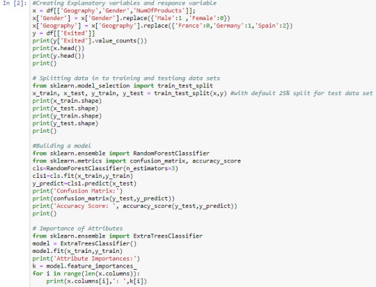
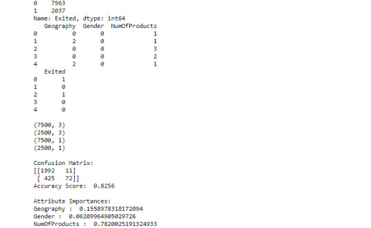
Observations: I built the forest with 3 trees using default 'Gini' criterion. And got the accuracy score around 82%. And also displayed importance of explanatory variables in the forest, which shows the attribute NumOfProducts is having most importance with score 0.79 and Gender is having least importance with score 0.05.

[ratnakishor-blog]

Week 1 - Machine Learning for Data Analysis - Running a Classification Tree

Building a model using two explanatory variables

Building a model using three explanatory variables

[ratnakishor-blog]

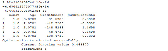
Week 4 - Regression Modeling in Practice - Test a Logistic Regression Model

[ratnakishor-blog]

Week 3 - Regression Modeling in Practice - Testing a Multiple Regression Model

[ratnakishor-blog]

Week 2 - Regression Modeling in Practice - Test a Basic Linear Regression Model

                                                                                                                          Testing the association between explanatory variable 'R&D Spend' and response variable 'Profit'.

Observations: 

F- Statistic is large and p-value is less than 0.05 so that we can reject null hypothesis and say there is significant association between R&D spend and Profit. 

Based on the parameters obtained from the model                                               Profit = 0.8543 * R&D Spend + 112000.

From R-squared value we can say around 94% variability can be observed in response variable Profit.

     Testing the association between explanatory variable 'Marketing Spend' and response variable 'Profit'.

Observations:

F- Statistic is large and p-value, 4.38e-10 is less than 0.05 so that we can reject null hypothesis and say there is significant association between R&D spend and Profit.

Based on the parameters obtained from the model                                                          Profit = 0.2465 * R&D Spend + 112000.

From R-squared value we can say around 56% variability can be observed in response variable Profit.

[ratnakishor-blog]

Week 1 - Regression Modeling in Practice - Writing about Data

Sample: The Iris flower data set or Fisher's Iris data set is a multivariate data set introduced by the British statistician and biologist Ronald Fisher in his 1936 paper  ‘The use of multiple measurements in taxonomic problems as an example of linear discriminant analysis’. It is sometimes called Anderson's Iris data set. 

Procedures: Edgar Anderson collected the data to quantify the morphologic variation of Iris flowers of three related species. Two of the three species were collected in the Gaspé Peninsula "all from the same pasture, and picked on the same day and measured at the same time by the same person with the same apparatus".

Measures: The data set consists of 50 samples from each of three species of Iris (Iris setosa, Iris virginica and Iris versicolor). Four features were measured from each sample: the length and the width of the sepals and petals, in centimeters. Based on the combination of these four features, Fisher developed a linear discriminant model to distinguish the species from each other.

[ratnakishor-blog]

Week 4 - Data Analysis Tools - Exploring Statistical Interactions

 Observations: Now we can say that in both the states, New Yark and California, there is a strong positive statistically significant association between R&D Spend and Profit.

   Observations: In both the cases we got high chi square value and P-value << 0.05, means that both the tests are statistically significant. And also from means and graphs we can say that the moderator variable does not have any influence on the relation between two variables.

     Observations: In both the cases we got high F-statistic value and P-value << 0.05, means that both the tests are statistically significant. And also from graphs we can say that who choose Cardio exercise and diet chart 0 will have good weight loss and who choose weights exercise and diet chart 1 will have good weight loss. That means in the association between Diet chart and Weight Loss, type of Exercise acts as a moderator.

[ratnakishor-blog]

Data Analysis Tools - Week 3 - Pearson Correlation

Data set: 50-Startups.csv

Code book:

Hypothesis:

Null Hypothesis H0: There is no association between the quantitative response variable Profit and quantitative explanatory variables R&D Spend, Administration and Marketing Spend.

Alternate Hypothesis Ha: There is a association between the quantitative response variable Profit and quantitative explanatory variables R&D Spend, Administration and Marketing Spend.

 Python code:

Observations: Here since Pearson correlation coefficient r = 0.97 and P-value  << 0.05  we can say there is a very strong positive statistically significant relation between R&D spend and profit. Since r2 = 0.94 there is a 94% of variability in profit can be predicted by R&D spend.

Observations: Here since Pearson correlation coefficient r = 0.2 and P-value  >  0.05  we can say there is a weak  positive  relation between Administration  spend and profit. Since r2 = 0.04 there is only 4% of variability in profit can be predicted by Administration spend

Observations: Here since Pearson correlation coefficient r = 0.74 and P-value  << 0.05  we can say there is strong positive statistically significant relation between  spend and profit. Since r2 = 0.56 there is a 56% of variability in profit can be predicted by Marketing spend

[ratnakishor-blog]

Data Analysis Tools - Week 2 - Chi square Test

Data Set: Churn-modelling.xlsx

Code book:

Hypothesis 1: Explanatory Variable with two levels

Null Hypothesis H0: There is no relation between gender and the customer churn i.e., the variables Gender and Exited are independent.

Alternate Hypothesis Ha: There is a relation between Gender and the Customer churn i.e., the variables Gender and Exited are dependent.

Code:

From the result of chi-square test it is clear that χ2 > 3.84 and P < 0.05 we can reject the null hypothesis and can say the customer churn is statistically related to gender of the customer.

 Hypothesis 2: Explanatory variable with more than two levels

Null Hypothesis H0: There is no relation between the number of products holding and the customer churn i.e., the variables NumOfProducts and Exited are independent.

Alternate Hypothesis Ha: There is a relation between number of products holding and the Customer churn i.e., the variables NumOfProducts and Exited are dependent.

Code:

From the result of chi-square test it is clear that χ2 > 3.84 and P < 0.05 we can reject the null hypothesis and can say the customer churn is statistically related to Number of products that customer holds.

Since our explanatory variable NumOfProducts has 4 levels need to go with post hoc test to know which groups are statistically different.

comp1v2   1.0   2.0

Exited            

1        1409   348

0        3675 4242

comp1v2        1.0        2.0

Exited                      

1        27.714398   7.581699

0        72.285602  92.418301

Chi-square value:  656.4492571317394

P-value:  8.841692150752575e-145

 comp2v3   2.0 3.0

Exited            

1         348 220

0        4242   46

comp2v3        2.0        3.0

Exited                      

1         7.581699  82.706767

0        92.418301  17.293233

Chi-square value:  1366.5872147076109

P-value:  3.829666674972014e-299

comp3v4  3.0 4.0

Exited          

1        220   60

0         46   0

comp3v4        3.0   4.0

Exited                  

1        82.706767  100.0

0        17.293233    0.0

Chi-square value:  10.695787090007627

P-value:  0.0010737977930260988

comp1v3   1.0 3.0

Exited            

1        1409 220

0        3675   46

comp1v3        1.0        3.0

Exited                      

1        27.714398  82.706767

0        72.285602  17.293233

Chi-square value:  358.3728983487756

P-value:  6.36623788337487e-80

comp1v4   1.0 4.0

Exited            

1        1409   60

0        3675   0

comp1v4        1.0   4.0

Exited                  

1        27.714398  100.0

0        72.285602    0.0

Chi-square value:  148.35121066056206

P-value:  3.975197582728242e-34

 comp2v4   2.0 4.0

Exited            

1         348   60

0        4242   0

comp2v4        2.0   4.0

Exited                  

1         7.581699  100.0

0        92.418301    0.0

Chi-square value:  620.4847809929802

P-value:  5.865690173058868e-137

[ratnakishor-blog]

Data Analysis Tools – Week 1 – ANOVA

Data Set: diet_exercise.xls

Code Book:

Hypothesis 1:

Null Hypothesis H0: There is no association between type of exercise and amount of weight loss (Means are significantly equal i.e., μcardio = μweights).

Alternate Hypothesis H1: There is a significant association between type of exercise and weight loss (Means are not significantly equal).

Hypothesis 2:

Null Hypothesis H0: There is no association between type of diet chat and amount of weight loss (Means are significantly equal i.e., μA = μB = μC = μD).

Alternate Hypothesis H1: There is a significant association between type of diet chart and weight loss (Means are not significantly equal).

Python Code:

From the OLS Regression Results F-statistic = 16.58 and P-value = 0.000221.

Since p-value <<  0.05 we can reject null hypothesis.

That is there is a significant association between type of exercise and weight loss.

From the OLS Regression Results F-statistic = 9.477 and P-value = 0.0038.

Since p-value <<  0.05 we can reject null hypothesis.

That is there is a significant association between type of diet chart and weight loss.

Tokay’s Honesty Significant Difference Post Hoc Test:

From above table we can say there is a significant difference between μA and μB & μA and μC i.e., μA ≠ μB and μA ≠ μC. And means of diet charts B and C are not much significantly different. Statistically both B and C charts results approximately same weight loss.

[ratnakishor-blog]

Week 4 Assignment - Visual Analysis

Data Set: Churn_modelling.csv

Research Question: What are the customer related factors associated with customer churns of the bank?

Importing Libraries and Reading Data Set:

Checking for missing data:

Uni-variate Analysis:

Observation: Above distribution is uni-modal and skewed right. From the histogram we can clearly say that there are more number of middle aged persons present in the bank.

Observation: Bank is having slightly more male customers than female customers.

Observation: Above analysis says that the bank is holding more number of customers from France.

Observation: CreditScore distribution is Unimodal and left skewed as there are higher frequencies at greater credit scores (Right side).

Observation: Here we can say that the bank is having a good number of customers with 5+ years of tenure.

Observation: Estimated salary is having Uniform distribution.

Bi-variate Analysis:

 Here the response Variable ‘Exited’ is Categorical and coded with 0 and 1.

Since the response variable is having two possible values as per requirement steps to be considered are

Step 1: Convert the response variable as type number.

Step 2: If exploratory variable is not categorical perform the binning for it.

Step 3: Display Categorical Vs Categorical chart.

Observation: Female customer churn is more than male customer churn.

Observation: Old aged people are more likely to leave the bank.

Observation: Customer churns are more in Germany.

[ratnakishor-blog]

Week 3 Assignment

For week 3 assignment i have selected a new data set and framed a new research question as this data set is having more scope to explore

Data Set: Churn_modelling

Research Question: Is Customer churn is associated with Customer personal information such as age, Gender, geography, tenure, Salary and number of products he is holding in bank?

My Program:

   Cell 1: Importing pandas, reading data set and displaying all variables in the data set.  

   Cell 2: Checking for missing data in the data set. 

   Cell 3: Frequency Distributions of some of selected variables

       Cell 3 output:                                                                      

Geography Frequency Distribution Germany    2509 France     5014 Spain      2477 Name: Geography, dtype: int64 Gender Frequency Distribution Male      5457 Female    4543 Name: Gender, dtype: int64 Tenure Frequency Distribution 2     1048 1     1035 7     1028 8     1025 5     1012 3     1009 4      989 9      984 6      967 10     490 0      413 Name: Tenure, dtype: int64 Age Frequency Distribution 24    132 32    418 40    432 48    168 56     70 64     37 72     21 80      3 88      1 25    154 33    442 41    366 49    147 57     75 65     18 73     13 81      4 18     22 26    200 34    447 42    321 50    134 58     67 66     35 74     18 82      1 19     27 27    209 35    474 43    297     ... 60     62 68     19 76     11 84      2 92      2 21     53 29    348 37    478 45    229 53     74 61     53 69     22 77     10 85      1 22     84 30    327 38    477 46    226 54     84 62     52 70     18 78      5 23     99 31    404 39    423 47    175 55     82 63     40 71     27 79      4 Name: Age, Length: 70, dtype: int64

   Cell 4 and 5: Creation of secondary variable and its frequency distribution 

   Cell 6 and 7: Grouping Age variable and its frequency distribution.

[ratnakishor-blog]

Week - 2 Assignment

My Program:

Output:

As the value_counts() function is having dropna = Flase, if the data set has any null values it might been shown in the output. Then we can say the data set does not have any missing values.

The class values are having equal frequency distribution. Each class has 50 observations.

[ratnakishor-blog]

Data Set Selection, Research Question and Hypothesis.

Step 1:

Data set selected: Iris Data Set.

Step 2:

Topic of Interest: Species of iris flower.

Step 3:

Code book for selected topic:

Step 4:

Second topic: Length and Width of the Sepals and Petals.

Step 5:

Addition of the second topic variables to code book

Step 6:

Literature Review:

The Iris flower data set or Fisher's Iris data set is a multivariate data set introduced by the British statistician and biologist Ronald Fisher in his 1936 paper  ‘The use of multiple measurements in taxonomic problems as an example of linear discriminant analysis’. It is sometimes called Anderson's Iris data set because Edgar Anderson collected the data to quantify the morphologic variation of Iris flowers of three related species. Two of the three species were collected in the Gaspé Peninsula "all from the same pasture, and picked on the same day and measured at the same time by the same person with the same apparatus".

The data set consists of 50 samples from each of three species of Iris (Iris setosa, Iris virginica and Iris versicolor). Four features were measured from each sample: the length and the width of the sepals and petals, in centimeters. Based on the combination of these four features, Fisher developed a linear discriminant model to distinguish the species from each other.

Step 7:

Research Question:

Is Iris Species is associated with length and width of the Sepals and Petals?

Hypothesis:

The Iris species type is associated with length and width of the Sepals and Petals.