regressionmodelinginpractice1

[regressionmodelinginpractice1]

Week 4

My initial question asked if there was an association between female employment rate and life expectancy. This week we are looking at logistic regression models and I considered additional explanatory variables of internet user rates and urban rates. 

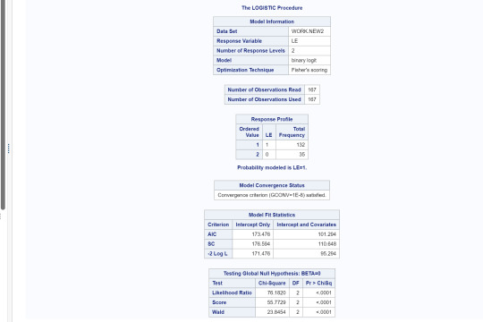
The output of the logistic models follows. It includes looking at just female employment rate, female employment rates and internet user rates, female employment rates and urban rates, and lastly female employment rates, internet user rates and urban rates. In each case, I centered the explanatory variables first and binned the response variable (life expectancy) into 2 categories- below 60 years old or not. 

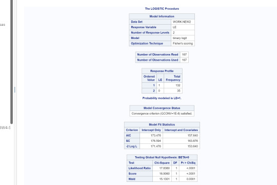
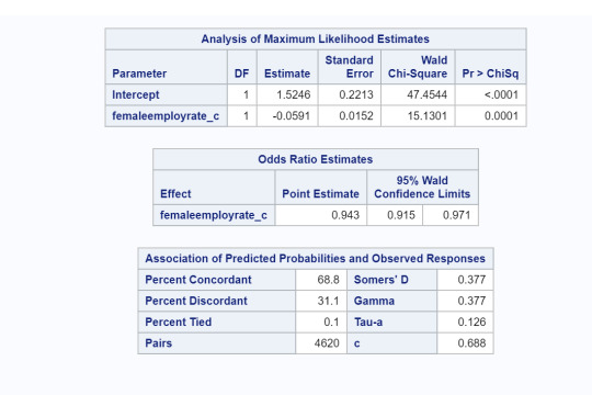
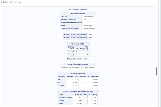
Interpretation:

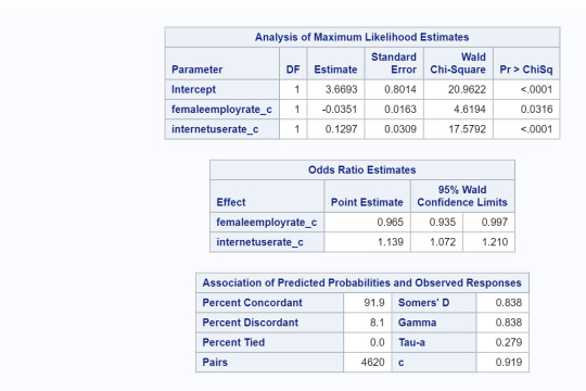
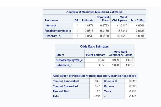
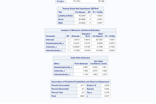
Female employment rates were significantly associated with life expectancy (OR=.943, 95% CI=9.15-.971, p=.0001). This implies since OR<1, as female employment rates increase, life expectancy above 60 years old is less likely. When adding the explanatory variable, internet user rate, we find that both female employment and internet user rates are both significantly associated with life expectancy. (OR=.965, 95% CI=.935-.997, p=.03, and OR=1.13, 95% CI=1.072-1.2, p=.0001, respectively). The OR for female employment rate relationship is the same as above but for internet user rates, since OR>1, implies that as internet user rates increase then life expectancy of above 60 years old is more likely. When considering female employment rate and urban rates, we find that both are statistically associated with life expectancy. (OR=.969, 95% CI=.939-1.0, p=.0487, and OR=1.055, 95% CI=1.03-1.08, p=.0001, respectively). However, when looking at all three together, we found that female employment rates and urban rates are no longer statistically significant in association with life expectancy above 60 years old but internet user rate is  (OR=.965, 95% CI=.935-.1, p=.057, OR=1.005, 95% CI=.974-1.38, p=.745,and OR=1.13, 95% CI=1.063-1.2, p=.0001, respectively). This implies that internet user rate confounds the relationship between female employment rates and urban rates with the response variable life expectancy above 60 years old. 

[regressionmodelinginpractice1]

Week 3

This week we are interpreting a multiple regression model. My initial explanatory variable is female employment rates and my response variable is life expectancy. My secondary explanatory variables were internet user rates and urban rates. 

My output from the multiple regression model is as follows. I first ran a linear model with no confounding variables. Then I ran a quadratic model to see if the data fit a polynomial better than a line. Then I added individually internet user rates, then urban rates, and finally both internet user rates and urban rates. For each of my three explanatory variables (female employment rates, internet user rates, and urban rates) I first centered them so that their mean was close to zero. 

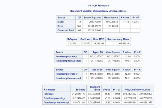
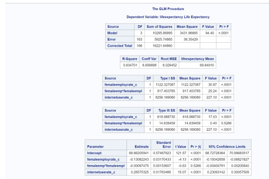
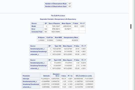
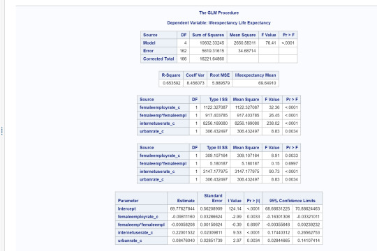
Interpretation of multiple regression models:

After adjusting for potential confounding factors (internet user rates and urban rates), female employment rate (Beta=-0.09, p=.0033) was significantly and negatively associated with life expectancy. Internet user rate (Beta=.22, p=.0001) and urban rate (Beta= .06, p= .0034) were both significant and positively associated with life expectancy after controlling for female employment rates. However, there was confounding issues when I ran them individually. Urban rates confound the relationship between female employment rates and life expectancy since when the regression model was run with just the urban rate added, female employment rate was no longer statistically significant (p=.231). 

Regression diagnostic plots

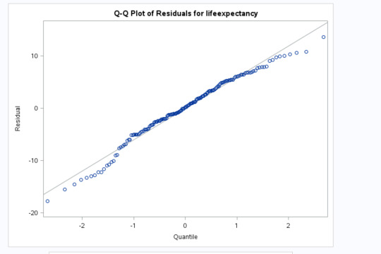
This q-q plot measures how much the residuals are normally distributed. In this plot, it looks like the residuals basically follow a line but deviate at the lower and higher quantiles. This could be because there are other confounding variables that I have not taken into consideration and that the curvilinearity is not completely controlled by the quadratic factor I found in my scatterplots. 

Standardized residuals for all observations

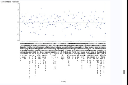
We notice that there are about 3 observations that fall outside 2.5 standard deviations. This is greater than 1% of all the observations (n=167).There are approximately 8 observations that fall outside 2 standard deviations. This is just less than 5% of all the observations. Since the first occurs, this tells us that the model is probably a poor fit of our observed values. This is probably contributed to leaving out an important explanatory variable. 

Leverage Plot

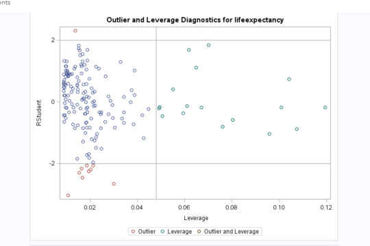
First, this shows us that we have many observations that have no leverage or effect on our model as they are close to 0. We have a few outliers (as seen in red) but they are close to 0 so they do not appear to influence our model. We have a few observations with high leverage which means they influence it in predicting the values for life expectancy. We have no observations that are both outlier and leverage the model. 

[regressionmodelinginpractice1]

Week 2

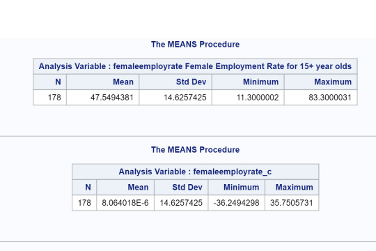
This week we are doing a simple linear regression model to test the association between the explanatory variable (female employment rate) and response variable (life expectancy). The first thing I did was center the quantitative explanatory variable. The code and output follow.

Code: 

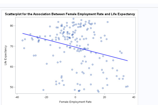
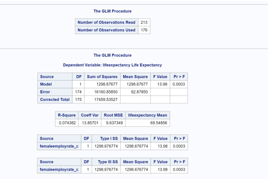
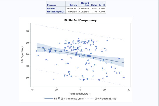
Conclusions: The results of the linear regression model indicated that female employment rate (centered at 0) was significantly and negatively associated with life expectancy. We got a beta=-.185 and a p-value of .0003<.05. Our regression line was y=69.55-.185x. Our r-squared value is .0743. This implies that about 7% of the variability of female employment rate can be predicted by life expectancy. 

[regressionmodelinginpractice1]

Week 1

My research question asks whether there is an association between female employment rates and life expectancy. 

Sample

The sample is from the GapMinder data subset. GapMinder is a collection of data sets that deal with social, economic, and environmental factors worldwide. Participants (N=215) represent the 192 UN members, an aggregate for Serbia and Montenegro, and 23 other countries of the world. The data analytics for this question include looking at the two specific indicators of female employment rates (N=178) and life expectancy (N=191) for each country that reported it.  For female employment rates the sample was taken from 2007 for female employees’ whose age was above 15 years old who had been employed during the previous year. For life expectancy, the sample was taken in 2011 and calculated as the average number of years a newborn child would live if current mortality patterns were to stay the same.

 Procedure

Data for GapMinder was collected by data reporting agencies. Data for female employment rate was collected by the International Labor Organization (https://www.ilo.org/global/statistics-and-databases/statistics-overview-and-topics/sdgs/lang--en/index.htm) during 2007 through country participation from countries’ national statistical offices (NSOs) and the Ministries of Labor. Data for life expectancy was collected through four sources: 1) Human Mortality Database, 2. World Population Prospects: 3. Publications and files by history prof. James C Riley and 4. Human Lifetable Database. (https://d396qusza40orc.cloudfront.net/phoenixassets/data-management-visualization/GapMinder%20Codebook%20.pdf) In each case, the data was collected by official government offices of the various countries who self-reported it to the various collecting agencies.

 Measures

The measure of female employment rate (quantitative explanatory variable) was drawn from data compiled by the International Labor Organization and made available for download through the GapMinder website (www.gapminder.org). It measures the number of female employees over age 15 who were employed the previous year.  The measure of life expectancy (quantitative response variable) was collected through four sources: 1) Human Mortality Database, 2. World Population Prospects: 3. Publications and files by history prof. James C Riley 4. Human Lifetable Database and made available for download through the GapMinder website (www.gapminder.org ). It measures the average number of years a newborn child would live if current mortality patterns were to stay the same. For the current analysis, the female employment rate was collapsed into four categories in order to make it a categorical variable. The four categories are: female employment rate <25%, 25-50%, 50-75%, and >75%.  Life expectancy remained a quantitative variable.