rwatson2020

[rwatson2020]

Capstone Milestone Assignment 1: Title and Introduction to the Research Question

Title - The association between tornado physical characteristics and direct economic losses.

Introduction to the Research Question

The purpose of this study was to identify whether a tornado’s physical characteristics, such as length and width while on the ground, correlated with the direct economic losses, such as property and crop damage or injuries and loss of life, of the impacted area. 

As a resident of Alabama, tornadic activity is an year long weather possibility. Having a better understanding on whether a tornado’s physical characteristics are correlated with the direct economic losses of the impacted areas will allow for more informed risk assessments of property investments in tornadic active areas. 

Understanding the correlation of direct losses resulting from the destruction of assets from the initial impact of the tornado leads to more informed decisions on the risks of investments in high tornadic areas.

[rwatson2020]

Peer-graded Assignment: Running a k-means Cluster Analysis - Week 4

A k-means cluster analysis was conducted to identify underlying subgroups of females based on their similarity on 2 variables that represent characteristics that could have an impact on infant mortality. Clustering variables included two quantitative variables measuring birth attendants present and number of living children. All clustering variables were standardized to have a mean of 0 and a standard deviation of 1.

Data were randomly split into a training set that included 70% of the observations (N=121) and a test set that included 30% of the observations (N=52). A series of k-means cluster analyses were conducted on the training data specifying k=1-9 clusters, using Euclidean distance. The variance in the clustering variables that was accounted for by the clusters (r-square) was plotted for each of the nine cluster solutions in an elbow curve to provide guidance for choosing the number of clusters to interpret.

Click to enlarge if logged in Tumblr or right click and open in new tab.

The elbow curve was inconclusive, suggesting that the 3, 5 and 6-cluster solutions might be interpreted. The results below are for an interpretation of the 3-cluster solution.  

A scatterplot of the first two canonical variables by cluster (Figure 2 shown below) indicated that the observations in clusters 1 and 2 overlap some but cluster 3 remained independent. 

In order to externally validate the clusters, an Analysis of Variance (ANOVA) was conducting to test for significant differences between the clusters on average years of education. A tukey test was used for post hoc comparisons between the clusters. Results indicated significant differences between the clusters on years of education. 

SOURCE CODE

[rwatson2020]

Peer-graded Assignment: Running a Lasso Regression Analysis - Week 3

A lasso regression analysis was conducted to identify a subset of variables from a pool of three quantitative predictor variables that best predicted a quantitative response variable measuring infant mortality.  Quantitative predictor variables include birth attendant present, average years of education, and average number of living children.  All predictor variables were standardized to have a mean of zero and a standard deviation of one.

Data were randomly split into a training set that included 70% of the observations (N=121) and a test set that included 30% of the observations (N=52). The least angle regression algorithm with k=10 fold cross validation was used to estimate the lasso regression model in the training set, and the model was validated using the test set. The change in the cross validation average (mean) squared error at each step was used to identify the best subset of predictor variables.

Plot 1, the average years of education = 0.16 and the average number of children = -0.12. 

Plot 2, the test data MSE = 0.107 which was less accurate than the training data MSE = 0.117. The training data R-square = 0.38 and the test data R-square = 0.46

Click to enlarge if logged in Tumblr or right click and open in new tab.

Plot 1 - Regression Coefficients Progression

Plot 2 - Change in the validation mean square error at each step

Code Output

Source Code

[rwatson2020]

Peer-graded Assignment: Running a Random Forest - Week 2

The following explanatory variables were included as possible contributors to a random forest evaluating Infant Mortality (my response variable), birth attendant present, average years education, and average number of living children.

The explanatory variables with the highest relative importance score was Average Number of Living Children at 0.47.  And the variable with the lowest important score is Birth Attendant Present at 0.07. The accuracy of the random forest was 81%

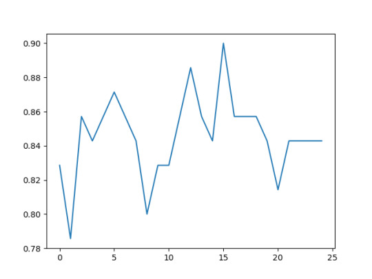
With only one tree the accuracy is about 78%, however it falls and then climbs again to about 90% with successive trees that are grown giving us low confidence that it may be appropriate to interpret a single decision tree for this data.

Click to enlarge if logged in Tumblr or right click and open in new tab.

PLOT

CODE OUTPUT

SOURCE CODE

[rwatson2020]

Peer-graded Assignment: Running a Classification Tree - Week 1

Click to enlarge if logged in Tumblr or right click and open in new tab.

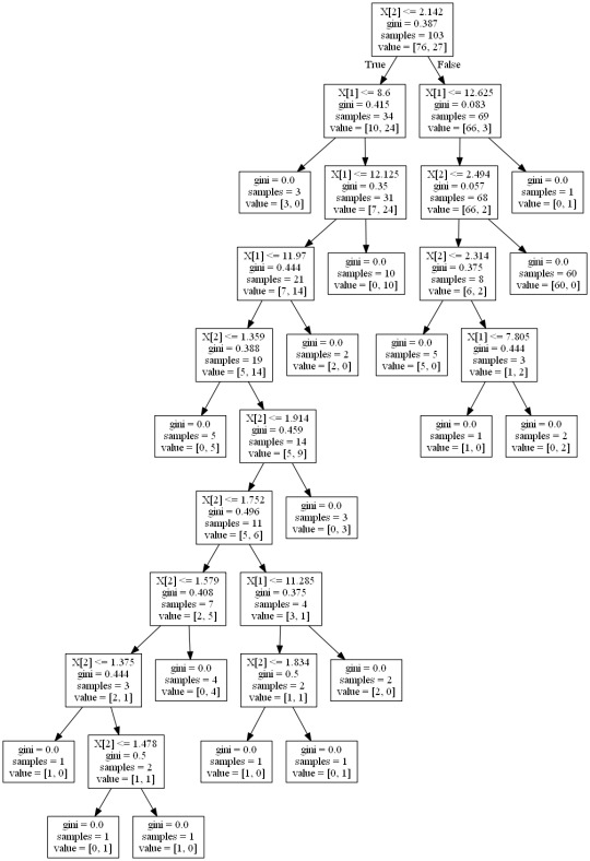
The following explanatory variables were included as possible contributors to a classification tree model evaluating Infant Mortality (my response variable), birth attendant present, average years education, and average number of living children. For Tree 3, the average number of living children was the first variable to separate the sample into two subgroups. Mothers with less than 2.177 living children were more likely to not have a birth attendant present and have lower years of education than females with higher education between 8.6 years and 12 + years. Sample size 34 with 84.28% accuracy. 

TREE 3

TREE 1

TREE 2

SOURCE CODE

[rwatson2020]

Peer-graded Assignment: Test a Logistic Regression Model - Week 4

Hypothesis: From 2000-2009, countries with higher female education level have a lower infant mortality rate than countries with lower female education level.

The effect of Years of Education on Infant Mortality: Years of Education regression is significant at a P value of less than .000 (p = 0.000). The probability of infant mortality is lower among those with higher Years of Education than among those less years of education. (OR = 0.494770). The odds ratio indicates that there's a 95% certainty that the odds ratio fall between 0.38 and 0.64 (CI = 0.381938-0.640933). Based on our model those with more Years of Education are anywhere from 0.38 and 0.64 times more likely to have less infant mortality than those with less Years of Education.

The effects of Average Number of Children, living, per Female on Infant Mortality: Average Number of Children regression is significant at a P value of less than .000 (p = 0.000). The probability of infant mortality is lower among those with greater Average Number of Children, living, per Female than those with less children (OR = 9.557892). The odds ratio indicates that there's a 95% certainty that the odds ratio fall between 4.03 and 22.64 (CI = 4.033392-22.649251). Based on our model those with greater Average Number of Children, living, per Female are anywhere from 4.03 and 22.64 times more likely to have less infant mortality than those with less Average Number of Children, living, per Female.

When we control for Years of Education: P value for Average Number of Children (p = 0.001) and Years of Education (p = 0.007) increased slightly. The greater number of living children are 5.07 times more likely to less infant mortality than with less number of children after controlling for Years of Education (OR = 5.072329). Also, females with higher number of years of education are .66 times more likely to have less infant mortality than daily females with less education, after controlling for the average number of living children (OR = 0.658087). The odds ratio indicates that there's a 95% certainty that the odds ratio fall between 0.48 and 0.89 for higher education (CI = 0.484585-0.893712) and there's a 95% certainty that the odds ratio fall between 2.02 and 12.70 for average number of living children (CI = 2.026320-12.697165).

The results supported my hypothesis: From 2000-2009, countries with higher female education level have a lower infant mortality rate than countries with lower female education level. My primary explanatory variable = Years of Education and response variable = Infant Mortality. There was no evidence of confounding for the association between Years of Education and Infant Mortality when adding a 3rd variable Birth Attendant Present it caused p values to be greater than .05. and coefficients to be negative, which means I should not use Birth Attendant Present as an explanatory variable.

Output of Logistic Regression Models - click to enlarge if logged in Tumblr or right click and open in new tab.

Source Code - click to enlarge if logged in Tumblr or right click and open in new tab.

[rwatson2020]

Regression Modeling in Practice Peer-graded Assignment: Test a Multiple Regression Model - Week 3

After adjusting for potential confounding factors – years of education and percentage of birth attendant present during birth, education (Beta= -3.51, p<.0001) was significantly and positively associated with lowering infant mortality. Birth attendant present was also significantly associated with lowering infant mortality rates, such that the rates of mortality were below 65 deaths per 1000 live births (Beta= -51.4, p<.0001). The infant mortality rate when years of education and birth attendants present are at their means is 36 out of every 100.

The results support my hypothesis: From 2000-2009, countries with higher female education level have a lower infant mortality rate than countries with lower female education level.

R-squared increased from 65.2% to 71.7%, evidence of confounding for the association between years of education and infant mortality when birth attendant present was factored in.

Q-Q plot shows that the residuals slightly follow a straight line. This indicates that the residuals did not follow perfect normal distribution.

Standardized residuals plot for all observations less than 1% of the observations has standardized residuals with an absolute value greater than 2.5, evidence that the level of error within the model is acceptable. That is the model is a fairly good fit to the observed data.

Leverage plot displays a few outliers, contents that have residuals greater than 2 or less than -2. This plot captures these outliers have a small or close to zero leverage values, meaning that although they are outlying observations, they do not have an undue influence on the estimation of the regression model. On the other hand, there are a few cases with higher than average leverage. But one in particular is more obvious in terms of having an influence on the estimation of the predicted value of infant mortality rate. This observation has a high leverage but is not an outlier. There aren’t any observations that are both high leverage and outliers.

OLS Regression Results & Regression Diagnostic Plots  - click to enlarge if logged in Tumblr or right click and open in new tab.

SOURCE CODE - click to enlarge if logged in Tumblr or right click and open in new tab.

[rwatson2020]

Regression Modeling in Practice Peer-graded Assignment: Test a Basic Linear Regression Model - Week 2

Question: Is Infant Mortality greater for births with or without birth attendants?

Dep. Variable: AVEINFMORT10YR No. Observations: 163

The results of the linear regression model indicated that % of birth attendants present was significantly associated with infant mortality rate.  p value = p<.0001  The best fit line of this graph is Infant Mortality rate = -0.7699 + 1.00 * AVEBIRTHATT10YR. 

CENTERED MEAN OUTPUT AND OLS REGRESSION OUTPUT -  click to enlarge if logged in Tumblr or right click and open in new tab.

Quantitative Explanatory Variable CENTERED

F-statistic: 1.642e+32 Prob (F-statistic): 0.00 - We can reject the null hypothesis and conclude that birth attendant rate is significantly associated with infant mortality rate.

coef - Intercept = -0.7699 and AVEBIRTHATT10YR = 1.0000 The best fit line of this graph is Infant Mortality rate = -0.7699 + 1.00 * AVEBIRTHATT10YR.

p value = p<.0001

R-squared: 1.000 Accounts for a perfect correlation in the response variable, Infant Mortality.

OLS REGRESSION OUTPUT (EXP Variable not centered) -  click to enlarge if logged in Tumblr or right click and open in new tab.

Quantitative Explanatory Variable NOT CENTERED

F-statistic: 326.3 Prob (F-statistic): 1.47e-40 (very small) - We can reject the null hypothesis and conclude that birth attendant rate is significantly associated with infant mortality rate.

coef - Intercept = 109.7632 and AVEBIRTHATT10YR = -93.7593 The best fit line of this graph is Infant Mortality rate = 109.76 + -93.76 * AVEBIRTHATT10YR.

p value = p<.0001

R-squared: 0.670 Accounts for about 67% of the variability we see in the response variable, Infant Mortality.

Scatterplot - click to enlarge if logged in Tumblr or right click and open in new tab.

SOURCE CODE - click to enlarge if logged in Tumblr or right click and open in new tab. 

[rwatson2020]

Regression Modeling in Practice  Peer-graded Assignment: Writing About Your Data - Week 1

Hypothesis -  From 2000-2009, countries with higher education levels of females have a lower infant mortality rate than countries with lower education level.

Sample

The samples are from Gapminder.org, founded in Stockholm by Ola Rosling, Anna Rosling Rönnlund and Hans Rosling, GapMinder is a non-profit venture promoting sustainable global development and achievement of the United Nations Millennium Development Goals. It seeks to increase the use and understanding of statistics about social, economic, and environmental development at local, national, and global levels. Since its conception in 2005, Gapminder has grown to include over 200 indicators, including gross domestic product, total employment rate, and estimated HIV prevalence. Gapminder contains data for all 192 UN members, aggregating data for Serbia and Montenegro. Additionally, it includes data for 24 other areas, generating a total of 215 areas. GapMinder collects data from a handful of sources, including the Institute for Health Metrics and Evaluation, US Census Bureau’s International Database, United Nations Statistics Division, and the World Bank.

The specific data resources used for this project include the Global Burden of Disease Study 2017 (GBD 2017) - Deaths of children during first year of life (per 1000 live births), Institute for Health Metrics and Evaluation - The average number of years of school attended by all women of reproductive age 15 to 44, including primary, secondary, and tertiary education, and The World Bank - Births attended by skilled health staff are the percentage of deliveries attended by personnel trained to give the necessary supervision, care, and advice to women during pregnancy, labor, and the postpartum period; to conduct deliveries on their own; and to care for newborns. Participants (N=195) represented the UN member countries sampled. The data analytic sample for this project included averaged data from 2000-2009 for countries with data reported for infant mortality, education of females ages 15-44, and birth attendant surveys (N=174).

Procedure

Data were collected by Unicef, Institute for Health Metrics and Evaluation, and the World Bank. It is compilation of estimates for infant mortality rates (per 1,000 born), means years in school (women of reproductive age 15 to 44), and births attended by skilled health staff (% of total) through civil registration, censuses and nationally representative sample surveys.

Measures

Infant mortality, deaths of children during first year of life, was assessed using the Global Burden of Disease Study 2017 (GBD 2017). Infant mortality was measured in a quantitative variable - percentage per 1,000 births recorded for the given country. Averaged from YR 2000 – YR 2009 and Categorized:1 = 0-10 deaths per 1000, 2 = 10-20 deaths per 1000, 3 = 20-30 deaths per 1000, 4 = 30-40 deaths per 1000, 5 = 40-50 deaths per 1000, 6 = 50-60 deaths per 1000, 7 = 60-80 deaths per 1000, 8 = 80-100 deaths per 1000 and  9 = 100-130 deaths per 1000.

The average number of years of school attended by all women of reproductive age 15 to 44 was assessed using Institute for Health Metrics and Evaluation (IHME). A Hand Up: Global Progress Toward Universal Education. Seattle, WA: IHME, 2015. The means years were measured in a quantitative variable by 0-15 years of education for females of reproductive age for the given country. Averaged from YR 2000 – YR 2009 and Categorized:1 = 0-1 Years education, 2 = 1-2 Years education, 3 = 2-4 Years education, 4 = 4-6 Years education, 5 = 6-8 Years education, 6 = 8-10 Years education, 7 = 10-12 Years education, and 8 = 12-15 Years education.

Births attended by skilled health staff was assessed by UNICEF, State of the World's Children, Childinfo, and Demographic and Health Surveys. The percentage of birth attended was measured as a quantitative variable by total numbers of births for the given country. Averaged from YR 2000 – YR 2009 Categorized:4  = 75-100 Percent, 3 = 50-75 Percent, 2 = 25-50 Percent, and 1 = 0-25 Percent. Additionally categorized as 1=YES (birth attendant present), 0=NO (no birth attendant present).

[rwatson2020]

Data Analysis Tools - Peer-graded Assignment: Correlation Coefficient with a Moderator - Week 4

Hypothesis -  From 2000-2009, countries with higher education levels of females have a lower infant mortality rate than countries with lower education level. I have completed 3 Pearson correlation coefficient graphs with a moderator.

Scatterplot for the association between mortality rates and birth attendants present for females with 4 years or less in education (LOW).

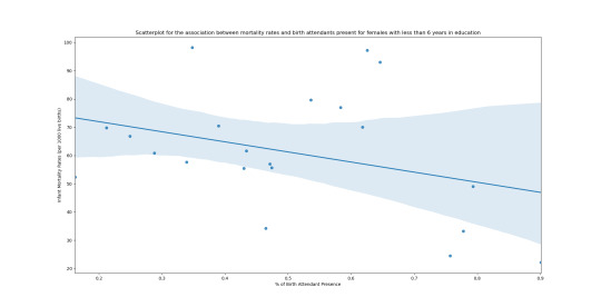
Scatterplot for the association between mortality rates and birth attendants present for females with less than 6 years in education (MID).

Scatterplot for the association between mortality rates and birth attendants present for females with more than 6 years in education (HIGH).

For scatterplot 1, the correlation coefficient is approximately -0.06 with a P value = 0.72 and small r squared = 0.0036  This tells us the relationship is NOT statistically significant. No association in lowering mortality rate with birth attendant is present.

For scatterplot 2, the correlation coefficient is approximately -0.34 with P value = 0.133 and small r squared = 0.1156  This tells us the relationship is NOT statistically significant. No association in lowering mortality rate with birth attendant is present.

For scatterplot 3, the correlation coefficient is approximately -0.72 with a very small P value and small r squared = 0.5184  This tells us the relationship IS statistically significant. 

Output and source code below - click to enlarge if logged in Tumblr or right click and open in new tab.

Scatterplot 1

Scatterplot 2

Scatterplot 3

Code Output

Source Code

[rwatson2020]

Data Analysis Tools - Peer-graded Assignment: Generating a Correlation Coefficient - Week 3

Hypothesis -  From 2000-2009, countries with higher education levels of females have a lower infant mortality rate than countries with lower education level.

I have completed 2 Pearson correlation coefficient graphs. 

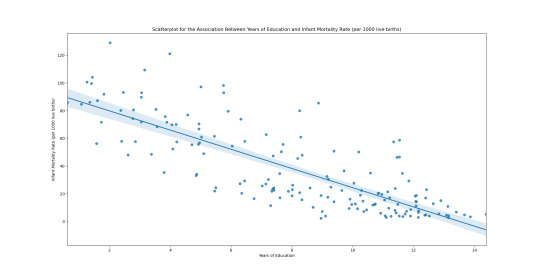
Scatterplot for the Association Between Years of Education and Infant Mortality Rate (per 1000 live births)

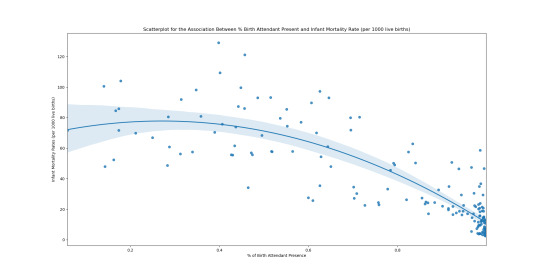
Scatterplot for the Association Between % Birth Attendant Present and Infant Mortality Rate (per 1000 live births)

For scatterplot 1, the correlation coefficient is approximately -0.81 with a very small P value.  This tells us the relationship is statistically significant.

For scatterplot 2, the correlation coefficient is approximately -0.82 with a very small P value.  This also tells us the relationship is statistically significant.

In support of my hypothesis, scatterplot 1 has small r squared = .66  If we know the years of education, we can predict 66% of the variability we will see in the rate of infant mortality.

Output and source code below - click to enlarge if logged in Tumblr or right click and open in new tab.

Scatterplot 1

Scatterplot 2

Output of correlation coefficient

Source code

[rwatson2020]

Data Analysis Tools - Peer-graded Assignment: Running a Chi-Square Test of Independence - Week 2

Hypothesis -  From 2000-2009, countries with higher education levels of females have a lower infant mortality rate than countries with lower education level.

I have completed 1 Chi-Square Test (Explanatory variable with 7 levels & Response variable with two levels) and Post Hoc Analysis.

Data set = 174 Countries

Sample n = 99 Countries with infant mortality rates of greater than 30% per 1,000 births.

Run a Chi-Square Test of Independence - 

Does the presence of a birth attendant affect infant mortality? Chi-Square Test of Independence revealed that among 7 explanatory variables of mortality rates groups for 99 countries with infant mortality rates of 30% or greater with a birth attendant present, there was little positive impact between 30% - 80% mortality rate.

X2 = 12.29, df 6, p= 0.055

Therefore, we would ACCEPT the null hypothesis - No association in mortality rate with birth attendant is present.

Output and source code below - click to enlarge if logged in Tumblr or right click and open in new tab.

Post Hoc Tests

Source Code

print ('+++++++++++++++++++++++++++++++++++++++++++++++++++++++++++++++++++++') print ('*** Completing Post Hoc Tests ***')

recode2 = {3: 3, 4: 4} sub2['COMP1v2']= sub2['GROUPVALUE10YRAVEMORT2'].map(recode2)

# contingency table of observed counts ct2=pandas.crosstab(sub2['BIRTHATT'], sub2['COMP1v2']) print (ct2)

# column percentages colsum=ct2.sum(axis=0) colpct=ct2/colsum print(colpct)

print ('chi-square value, p value, expected counts') cs2= scipy.stats.chi2_contingency(ct2) print (cs2)

recode3 = {3: 3, 5: 5} sub2['COMP1v6']= sub2['GROUPVALUE10YRAVEMORT2'].map(recode3)

# contingency table of observed counts ct3=pandas.crosstab(sub2['BIRTHATT'], sub2['COMP1v6']) print (ct3)

# column percentages colsum=ct3.sum(axis=0) colpct=ct3/colsum print(colpct)

print ('chi-square value, p value, expected counts') cs3= scipy.stats.chi2_contingency(ct3) print (cs3)

recode4 = {3: 3, 6: 6} sub2['COMP1v14']= sub2['GROUPVALUE10YRAVEMORT2'].map(recode4)

# contingency table of observed counts ct4=pandas.crosstab(sub2['BIRTHATT'], sub2['COMP1v14']) print (ct4)

# column percentages colsum=ct4.sum(axis=0) colpct=ct4/colsum print(colpct)

print ('chi-square value, p value, expected counts') cs4= scipy.stats.chi2_contingency(ct4) print (cs4)

recode5 = {3: 3, 7: 7} sub2['COMP1v22']= sub2['GROUPVALUE10YRAVEMORT2'].map(recode5)

# contingency table of observed counts ct5=pandas.crosstab(sub2['BIRTHATT'], sub2['COMP1v22']) print (ct5)

# column percentages colsum=ct5.sum(axis=0) colpct=ct5/colsum print(colpct)

print ('chi-square value, p value, expected counts') cs5= scipy.stats.chi2_contingency(ct5) print (cs5)

recode6 = {3: 3, 8: 8} sub2['COMP1v30']= sub2['GROUPVALUE10YRAVEMORT2'].map(recode6)

# contingency table of observed counts ct6=pandas.crosstab(sub2['BIRTHATT'], sub2['COMP1v30']) print (ct6)

# column percentages colsum=ct6.sum(axis=0) colpct=ct6/colsum print(colpct)

print ('chi-square value, p value, expected counts') cs6= scipy.stats.chi2_contingency(ct6) print (cs6)

recode7 = {3: 3, 9: 9} sub2['COMP2v6']= sub2['GROUPVALUE10YRAVEMORT2'].map(recode7)

# contingency table of observed counts ct7=pandas.crosstab(sub2['BIRTHATT'], sub2['COMP2v6']) print (ct7)

# column percentages colsum=ct7.sum(axis=0) colpct=ct7/colsum print(colpct)

print ('chi-square value, p value, expected counts') cs7=scipy.stats.chi2_contingency(ct7) print (cs7) print ('+++++++++++ END OF Running Week 2 Program Assignment ++++++++++++')

[rwatson2020]

Data Analysis Tools - Peer-graded Assignment: Running an analysis of variance - Week 1

Hypothesis -  From 2000-2009, countries with higher education levels of females have a lower infant mortality rate than countries with lower education level.

I have completed 2 ANOVAs (Explanatory variables with more than 2 levels &  Explanatory variables with two levels)

Data set = 174 Countries

Sample n = 73 Countries with infant mortality rates of greater than 40% per 1,000 births.

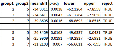
Multiple Variable Question: Does female education level affect infant mortality? Analysis of Variance (ANOVA) revealed that among 7 explanatory variables of education levels for countries with infant mortality rates of 40% or greater -

The Prob (F-statistic): 3.84e-05 

Therefore, we would REJECT the null hypothesis - No difference in mortality rate among the different levels of completed education. Post Hoc test comparison (Tukey) provided in next section.

Output and source code below - click to enlarge if logged in Tumblr or right click and open in new tab..

Model Interpretation for post hoc ANOVA results:

ANOVA revealed that females with 2 (1-2 years) & 3 (2-4 years) of formal education had higher rates of infant mortality as compared to females with 6 years or more formal education. 

2 Variable Question: Does having a birth attendant present decrease infant mortality?  Analysis of Variance (ANOVA) revealed that NO presence of a birth attendant had a slightly higher infant mortality rates (Mean = 75.57, s.d. ± 18.45) than those with the presence of a birth attendant (Mean = 65.19,  s.d. ± 23.01) 

The Prob (F-statistic): 0.179

Therefore, we would ACCEPT the null hypothesis - No significant difference in mortality rate with or without birth attendant.

Output and source code below - click to enlarge if logged in Tumblr or right click and open in new tab..

[rwatson2020]

Data Management and Visualization - Peer-graded Assignment: Creating graphs for your data Week 4

Questions -

·         Does female education level affect child mortality (0-5 years)?

Variable 1 =  meanyrsinschoolfemale (The average number of years of school attended by all women of reproductive age 14 to 44, including primary, secondary, and tertiary education. Averaged from YR 2000 – YR 2009)

Variable 2 =  Infantmortalityunder1 (Deaths of children during first year of life (per 1000 live births)Averaged from YR 2000 – YR 2009)

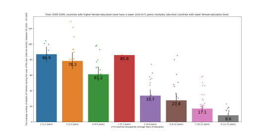
Hypothesis - From 2000-2009, countries with higher female education level have a lower child (0-5 years) mortality rate than countries with lower female education level.

Univariate bar graph for 1st variable

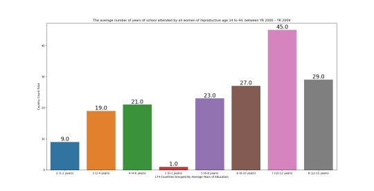
The average number of years of school attended by all women of reproductive age 14 to 44, between YR 2000 – YR 2009 This bar graph displays a bimodal distribution shape with the spread consisting of approximate minimum of .62 years of education (0-1 years education) to maximum 14.38 years of education (12-15 years). Approximate range of 13.76 years. The center mean is 8.32 years. The standard deviation is 3.6 years.

Univariate bar graph for 2nd variable

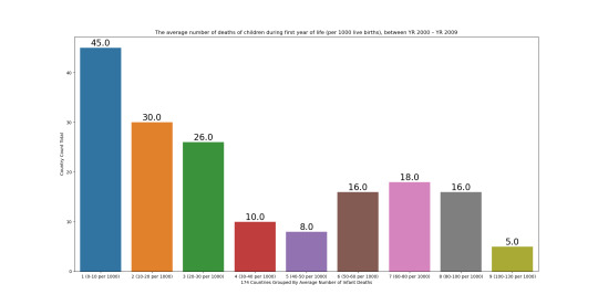
The average number of deaths of children during first year of life (per 1000 live births), between YR 2000 – YR 2009 This bar graph displays a bimodal distribution shape with the spread consistenting of approximate minimum of 2.47 deaths per 1,000 births to maximum 129.00 deaths per 1,000 births The center mean is 36 deaths per 1,000 births. The standard deviation is 31 deaths per 1,000 births.

Bivariate bar and scatter graph displaying the association between Average Number of Years Education (explanatory variable) and Infant Mortality Rate (response variable)

This graph displays that out of 174 countries surveyed, the 50 countries with females of reproductive age 14 to 44, between YR 2000 – YR 2009, with less than 6 years of education had the highest averages of infant mortality rates - 78 deaths per 1,000 births as compaired to countires with females of reproductive age 14 to 44, between YR 2000 – YR 2009, with more than 6 years of education - 22 deaths per 1,000 births.

Hypothesis - From 2000-2009, countries with higher female education level have a lower child (0-5 years) mortality rate than countries with lower female education level.

Week 3 Script

# -*- coding: utf-8 -*- """ Created on Thu Dec 17 16:55:49 2020

@author: Rebecca Watson - Data Management and Visualization Course """

# Import the libraries import pandas import numpy import seaborn import matplotlib.pyplot as plt

#Set PANDAS to show all columns in DataFrame pandas.set_option('display.max_columns', None) #Set PANDAS to show all rows in DataFrame pandas.set_option('display.max_rows', None)

# Import the dataset data = pandas.read_csv('CombinedData3.csv', low_memory=False)

#upper-case all DataFrame column names - place afer code for loading data aboave data.columns = list(map(str.upper, data.columns))

# bug fix for display formats to avoid run time errors - put after code for loading data above #pandas.set_option('display.float_format', lambda x:'%f'%x)

print ('!!!! Demonstrating displaying columns and rows of dataset !!!!')

print (len(data.columns)) # number of variables (columns) print (len(data)) #number of observations (rows) #print("\ntypes of data:\n", data.dtypes, sep="")

# setting variables to numeric data['10YRAVERAGEEDU'] = pandas.to_numeric(data['10YRAVERAGEEDU']) data['10YRAVEINFMORT'] = pandas.to_numeric(data['10YRAVEINFMORT'])

print ('')

sub1 = data[["COUNTRY", "10YRAVERAGEEDU", "10YRAVEINFMORT"]]

#make a copy of my new subsetted data sub2 = sub1.copy()

print(sub2)

# remove rows with missing values sub9 = sub2.dropna() subclean = sub9.copy()

# print data summary (of numeric variables) print(subclean.describe()) print ('')

print ('') print ('+++++++++++++++++++++++++++++++++++++++++++++++++++++++++++++++++++++') print ('')

# Import the libraries import pandas import numpy import seaborn import matplotlib.pyplot as plt

#Set PANDAS to show all columns in DataFrame pandas.set_option('display.max_columns', None) #Set PANDAS to show all rows in DataFrame pandas.set_option('display.max_rows', None)

# Import the dataset data = pandas.read_csv('CombinedData2.csv', low_memory=False)

#upper-case all DataFrame column names - place afer code for loading data aboave data.columns = list(map(str.upper, data.columns))

# bug fix for display formats to avoid run time errors - put after code for loading data above #pandas.set_option('display.float_format', lambda x:'%f'%x)

# setting variables to numeric data['10YRAVERAGEEDU'] = pandas.to_numeric(data['10YRAVERAGEEDU']) data['10YRAVEBIRTHATT'] = pandas.to_numeric(data['10YRAVEBIRTHATT']) data['10YRAVEINFMORT'] = pandas.to_numeric(data['10YRAVEINFMORT'])

print ('') print ('**************CHARTS************************') print ('')

# Univariate bar graph for 1st variable # First change format from numeric to categorical # data["GROUPVALUE10YRAVEEDU"] = data["GROUPVALUE10YRAVEEDU"].astype('category')

# plt.figure(figsize=(8, 6)) # splot = seaborn.countplot(x="GROUPVALUE10YRAVEEDU", data=data) # for p in splot.patches: #     splot.annotate(format(p.get_height(), '.1f'), #                    (p.get_x() + p.get_width() / 2., p.get_height()), #                    ha = 'center', va = 'center', #                    size=20, #                    xytext = (0, 10), #                    textcoords = 'offset points') # plt.xlabel('174 Countries Grouped By Average Years of Education') # plt.ylabel('Country Count Total') # plt.title('The average number of years of school attended by all women of reproductive age 14 to 44, between YR 2000 – YR 2009')

# Univariate bar graph for 2nd variable # First change format from numeric to categorical data["GROUPVALUE10YRAVEMORT"] = data["GROUPVALUE10YRAVEMORT"].astype('category') plt.figure(figsize=(8, 6)) splot = seaborn.countplot(x="GROUPVALUE10YRAVEMORT", data=data) for p in splot.patches:    splot.annotate(format(p.get_height(), '.1f'),                   (p.get_x() + p.get_width() / 2., p.get_height()),                   ha = 'center', va = 'center',                   size=20,                   xytext = (0, 10),                   textcoords = 'offset points') plt.xlabel('174 Countries Grouped By Average Number of Infant Deaths') plt.ylabel('Country Count Total') plt.title('The average number of deaths of children during first year of life (per 1000 live births), between YR 2000 – YR 2009')

# plt.figure(figsize=(8, 6)) # splot = seaborn.barplot(x ='GROUPVALUE10YRAVEEDU', y ='10YRAVEINFMORT', data=data) # seaborn.stripplot(x ='GROUPVALUE10YRAVEEDU', y ='10YRAVEINFMORT', data=data) # for p in splot.patches: #     splot.annotate(format(p.get_height(), '.1f'), #                    (p.get_x() + p.get_width() / 2., p.get_height()), #                    ha = 'center', va = 'center', #                    size=20, #                    xytext = (0, -20), #                    textcoords = 'offset points') # plt.xlabel('174 Countries Grouped By Average Years of Education') # plt.ylabel('The average number of deaths of children during first year of life (per 1000 live births), between YR 2000 – YR 2009') # plt.title('From 2000-2009, countries with higher female education level have a lower child (0-5 years) mortality rate than countries with lower female education level.')

print ('+++++++++++ END OF Running Week 4 Program Assignment ++++++++++++')

[rwatson2020]

Data Management and Visualization - Peer-graded Assignment: Making Data Management Decisions Week 3

Week 3 Script

# -*- coding: utf-8 -*-

"""

Created on Thu Dec 17 16:55:49 2020

@author: Rebecca Watson - Data Management and Visualization Course

"""

# Import the libraries

import pandas

import numpy

# Import the dataset

data = pandas.read_csv('CombinedData2.csv', low_memory=False)

#upper-case all DataFrame column names - place afer code for loading data aboave

data.columns = list(map(str.upper, data.columns))

# bug fix for display formats to avoid run time errors - put after code for loading data above

#pandas.set_option('display.float_format', lambda x:'%f'%x)

print ('!!!! Demonstrating displaying columns and rows of dataset !!!!')

print (len(data.columns)) # number of variables (columns)

print (len(data)) #number of observations (rows)

#print("\ntypes of data:\n", data.dtypes, sep="")

# setting variables to numeric

data['10YRAVERAGEEDU'] = pandas.to_numeric(data['10YRAVERAGEEDU'])

data['10YRAVEBIRTHATT'] = pandas.to_numeric(data['10YRAVEBIRTHATT'])

data['10YRAVEINFMORT'] = pandas.to_numeric(data['10YRAVEINFMORT'])

#Set missing data to NAN

data['GROUPVALUE10YRAVEBIRTHATT2']=data['GROUPVALUE10YRAVEBIRTHATT2'].replace(9, numpy.nan)

print ('')

print ('+++++++++++++++++++++++++++++++++++++++++++++++++++++++++++++++++++++')

print ('')

print ('+++++++++++++++++++++ Demonstrating Grouping Data - Identifying Missing Data +++++++++++++++++++++')

print ('')

print ('# of Countries Average number of Live Births Attended by Health Professionals from 2000-2009')

ct3 = data.groupby('GROUPVALUE10YRAVEBIRTHATT').size()

print(ct3)

print (len(data['GROUPVALUE10YRAVEBIRTHATT'])) # add number of observations (rows)

print ('')

print ('% of Countries Average number of Live Births Attended by Health Professionals from 2000-2009')

pt3 = data.groupby('GROUPVALUE10YRAVEBIRTHATT').size() * 100 / len(data)

print(pt3)

print (len(data['GROUPVALUE10YRAVEBIRTHATT'])) # add number of observations (rows)

print ('+++++++++++++++++++++++++++++++++++++++++++++++++++++++++++++++++++++')

print ('')

print ('+++++++++++++++++++++ Demonstrating Subset Data - Removing Missing Data +++++++++++++++++++++')

print ('')

sub1 = data[["COUNTRY", "10YRAVERAGEEDU", "10YRAVEINFMORT", "10YRAVEBIRTHATT"]]

#make a copy of my new subsetted data

sub2 = sub1.copy()

print(sub2)

# remove rows with missing values

sub9 = sub2.dropna()

subclean = sub9.copy()

# print data summary (of numeric variables)

print(subclean.describe())

print ('')

print ('+++++++++++++++++++++++++++++++++++++++++++++++++++++++++++++++++++++')

print ('')

print ('+++++++++++++++++++++ Demonstrating Binning +++++++++++++++++++++')

print ('')

# # create six equal-sized groups per variable

subclean['GroupEducation'] = pandas.qcut(subclean['10YRAVERAGEEDU'], 6)

subclean['GroupMortality'] = pandas.qcut(subclean['10YRAVEINFMORT'], 6)

subclean['GroupBirthAtt'] = pandas.qcut(subclean['10YRAVEBIRTHATT'], 6)

# print the first five rows of the data

print("First five rows of the data:\n", subclean.head())

print ('')

print ('+++++++++++++++++++++++++++++++++++++++++++++++++++++++++++++++++++++')

print ('')

print ('+++++++++++ Demonstrating Grouping ++++++++++++')

print ('')

#ADDING MORE DESCRIPTIVE TITLES

print('/GROUPVALUE10YRAVEEDU/ Total Count of Countries By Average Years of Education females 14-44 from YRS 2000-2009')

c1 = data['GROUPVALUE10YRAVEEDU'].value_counts(sort=True)

print (c1)

print (len(data['GROUPVALUE10YRAVEEDU'])) # add number of observations (rows)

print ('')

print('/GROUPVALUE10YRAVEEDU/ Percentages of Countries By Average Years of Education females 14-44 from YRS 2000-2009')

p1 = data['GROUPVALUE10YRAVEEDU'].value_counts(sort=True, normalize=True)

print (p1)

print ('')

print ('/GROUPVALUE10YRAVEMORT/ Total Count of Countries By Average Infant Mortality Rates from YRS 2000-2009')

c2 = data["GROUPVALUE10YRAVEMORT"].value_counts(sort=True)

print (c2)

print (len(data['GROUPVALUE10YRAVEMORT'])) # adding number of observations (rows)

print ('')

print ('/GROUPVALUE10YRAVEMORT/ Percentages of Countries By Average Infant Mortality Rates from YRS 2000-2009')

p2 = data["GROUPVALUE10YRAVEMORT"].value_counts(sort=True, normalize=True)

print (p2)

print ('')

print ('/GROUPVALUE10YRAVEBIRTHATT/ Total Count of Countries By Average number of Live Births Attended by Health Professionals from YRS 2000-2009')

c3 = data["GROUPVALUE10YRAVEBIRTHATT"].value_counts(sort=True)

print (c3)

print (len(data['GROUPVALUE10YRAVEBIRTHATT'])) # add number of observations (rows)

print ('')

print ('/GROUPVALUE10YRAVEBIRTHATT/ Percentages of Countries By Average number of Live Births Attended by Health Professionals from YRS 2000-2009 ')

p3 = data["GROUPVALUE10YRAVEBIRTHATT"].value_counts(sort=True, normalize=True)

print (p3)

print ('')

print ('+++++++++++ END OF Running Week 3 Program Assignment ++++++++++++')

@@@@@@@@@@@@@@@@@@@@@@@@@@

OUTPUT FROM CODE

runfile('C:/Users/Rebecca/Desktop/Data Course/Python Files/Week3Script.py', wdir='C:/Users/Rebecca/Desktop/Data Course/Python Files') !!!! Demonstrating displaying columns and rows of dataset !!!! 8 174

+++++++++++++++++++++++++++++++++++++++++++++++++++++++++++++++++++++

+++++++++++++++++++++ Demonstrating Grouping Data - Identifying Missing Data +++++++++++++++++++++

# of Countries Average number of Live Births Attended by Health Professionals from 2000-2009 GROUPVALUE10YRAVEBIRTHATT 1 (0-25 Percent)       10 2 (25-50 Percent)      25 3 (50-75 Percent)      25 4 (75-100 Percent)    103 9 Unknown              11 dtype: int64 174

% of Countries Average number of Live Births Attended by Health Professionals from 2000-2009 GROUPVALUE10YRAVEBIRTHATT 1 (0-25 Percent)       5.747126 2 (25-50 Percent)     14.367816 3 (50-75 Percent)     14.367816 4 (75-100 Percent)    59.195402 9 Unknown              6.321839 dtype: float64 174 +++++++++++++++++++++++++++++++++++++++++++++++++++++++++++++++++++++

+++++++++++++++++++++ Demonstrating Subset Data - Removing Missing Data +++++++++++++++++++++

           COUNTRY  10YRAVERAGEEDU  10YRAVEINFMORT  10YRAVEBIRTHATT 0          Ethiopia            1.73           71.73         0.059000 1              Chad            1.26          100.63         0.140500 2             Nepal            2.61           48.05         0.143250 3        Bangladesh            4.08           52.37         0.162429 4             Niger            1.07           84.62         0.167000 ..              ...             ...             ...              ... 169         Belgium           12.19            4.17              NaN 170          Israel           12.86            4.64              NaN 171           Spain           10.33            4.81              NaN 172  United Kingdom           12.83            5.11              NaN 173          Greece           11.82            5.24              NaN

[174 rows x 4 columns]       10YRAVERAGEEDU  10YRAVEINFMORT  10YRAVEBIRTHATT count      163.000000      163.000000       163.000000 mean         8.095153       37.579509         0.769883 std          3.587864       30.809262         0.268889 min          0.620000        2.470000         0.059000 25%          4.980000       12.410000         0.558375 50%          8.590000       24.520000         0.922333 75%         11.230000       57.890000         0.987821 max         14.380000      129.000000         0.999100

+++++++++++++++++++++++++++++++++++++++++++++++++++++++++++++++++++++

+++++++++++++++++++++ Demonstrating Binning +++++++++++++++++++

First five rows of the data:       COUNTRY  10YRAVERAGEEDU  ...  GroupMortality                  GroupBirthAtt 0    Ethiopia            1.73  ...  (50.25, 71.93]  (0.057999999999999996, 0.448] 1        Chad            1.26  ...  (71.93, 129.0]  (0.057999999999999996, 0.448] 2       Nepal            2.61  ...  (24.52, 50.25]  (0.057999999999999996, 0.448] 3  Bangladesh            4.08  ...  (50.25, 71.93]  (0.057999999999999996, 0.448] 4       Niger            1.07  ...  (71.93, 129.0]  (0.057999999999999996, 0.448]

[5 rows x 7 columns]

+++++++++++++++++++++++++++++++++++++++++++++++++++++++++++++++++++++

+++++++++++ Demonstrating Grouping ++++++++++++

/GROUPVALUE10YRAVEEDU/ Total Count of Countries By Average Years of Education females 14-44 from YRS 2000-2009 7 (10-12 years)    45 8 (12-15 years)    29 6 (8-10 years)     27 5 (6-8 years)      23 4 (4-6 years)      21 3 (2-4 years)      19 2 (1-2 years)       9 1 (0-1 years)       1 Name: GROUPVALUE10YRAVEEDU, dtype: int64 174

/GROUPVALUE10YRAVEEDU/ Percentages of Countries By Average Years of Education females 14-44 from YRS 2000-2009 7 (10-12 years)    0.258621 8 (12-15 years)    0.166667 6 (8-10 years)     0.155172 5 (6-8 years)      0.132184 4 (4-6 years)      0.120690 3 (2-4 years)      0.109195 2 (1-2 years)      0.051724 1 (0-1 years)      0.005747 Name: GROUPVALUE10YRAVEEDU, dtype: float64

/GROUPVALUE10YRAVEMORT/ Total Count of Countries By Average Infant Mortality Rates from YRS 2000-2009 1 (0-10 per 1000)       45 2 (10-20 per 1000)      30 3 (20-30 per 1000)      26 7 (60-80 per 1000)      18 6 (50-60 per 1000)      16 8 (80-100 per 1000)     16 4 (30-40 per 1000)      10 5 (40-50 per 1000)       8 9 (100-130 per 1000)     5 Name: GROUPVALUE10YRAVEMORT, dtype: int64 174

/GROUPVALUE10YRAVEMORT/ Percentages of Countries By Average Infant Mortality Rates from YRS 2000-2009 1 (0-10 per 1000)       0.258621 2 (10-20 per 1000)      0.172414 3 (20-30 per 1000)      0.149425 7 (60-80 per 1000)      0.103448 6 (50-60 per 1000)      0.091954 8 (80-100 per 1000)     0.091954 4 (30-40 per 1000)      0.057471 5 (40-50 per 1000)      0.045977 9 (100-130 per 1000)    0.028736 Name: GROUPVALUE10YRAVEMORT, dtype: float64

/GROUPVALUE10YRAVEBIRTHATT/ Total Count of Countries By Average number of Live Births Attended by Health Professionals from YRS 2000-2009 4 (75-100 Percent)    103 3 (50-75 Percent)      25 2 (25-50 Percent)      25 9 Unknown              11 1 (0-25 Percent)       10 Name: GROUPVALUE10YRAVEBIRTHATT, dtype: int64 174

/GROUPVALUE10YRAVEBIRTHATT/ Percentages of Countries By Average number of Live Births Attended by Health Professionals from YRS 2000-2009 4 (75-100 Percent)    0.591954 3 (50-75 Percent)     0.143678 2 (25-50 Percent)     0.143678 9 Unknown             0.063218 1 (0-25 Percent)      0.057471 Name: GROUPVALUE10YRAVEBIRTHATT, dtype: float64

+++++++++++ END OF Running Week 3 Program Assignment ++++++++++++

@@@@@@@@@@@@@@@@@@@@@@@@@@

Questions -

·         Does female education level affect child mortality (0-5 years)?

·         Is female education level associated with higher births attended by qualified health professional thus decreasing child mortality?

·         Is female education associated with a change in total fertility rate?

Hypothesis (revised 20DEC2020) -

From 2000-2009, countries with higher female education level have a lower child (0-5 years) mortality rate than countries with lower female education level.

VARIABLES

10YRAVERAGEEDU  10YRAVEINFMORT  10YRAVEBIRTHATT 

Data from Countries Average number of Live Births Attended by Health Professionals from 2000-2009 had missing data which I eliminated with this week’s script.

I binned each of my variables into six (6) equal sized groups.

 The data was sub-set to the lowest 5 educated countries to begin supporting my hypothesis. 

[rwatson2020]

Data Management and Visualization - Peer-graded Assignment: Running Your First Program - Week 2

Week 2 Script (Python 3.8)

# -*- coding: utf-8 -*- """ Created on Thu Dec 17 16:55:49 2020

@author: Rebecca Watson - Data Management and Visualization Course """

# Import the libraries import pandas import numpy

# Import the dataset data = pandas.read_csv('CombinedData.csv', low_memory=False)

#upper-case all DataFrame column names - place afer code for loading data aboave data.columns = list(map(str.upper, data.columns))

# bug fix for display formats to avoid run time errors - put after code for loading data above #pandas.set_option('display.float_format', lambda x:'%f'%x)

print ('!!!! Demonstrating displaying columns and rows of dataset !!!!')

print (len(data.columns)) # number of variables (columns) print (len(data)) #number of observations (rows) print ('')

# setting variables to numeric data['10YRAVERAGEEDU'] = pandas.to_numeric(data['10YRAVERAGEEDU']) data['10YRAVEBIRTHATT'] = pandas.to_numeric(data['10YRAVEBIRTHATT']) data['2000INFMORTPER1K'] = pandas.to_numeric(data['2000INFMORTPER1K']) data['10YRAVEINFMORT'] = pandas.to_numeric(data['10YRAVEINFMORT'])

print('++ Demonstrating Counts and Percentages of each Variable - No labels ++') # Counts and percentages (i.e. frequency distributions) for each variable print ('')

c1 = data["GROUPVALUE10YRAVEEDU"].value_counts(sort=True) print (c1) print (len(data['GROUPVALUE10YRAVEEDU'])) # add number of observations (rows) print ('')

p1 = data["GROUPVALUE10YRAVEEDU"].value_counts(sort=True, normalize=True) print (p1) print ('')

c2 = data["GROUPVALUE10YRAVEMORT"].value_counts(sort=True) print (c2) print (len(data['GROUPVALUE10YRAVEMORT'])) # add number of observations (rows) print ('')

p2 = data["GROUPVALUE10YRAVEMORT"].value_counts(sort=True, normalize=True) print (p2) print ('')

c3 = data["GROUPVALUE10YRAVEBIRTHATT"].value_counts(sort=True) print (c3) print (len(data['GROUPVALUE10YRAVEBIRTHATT'])) # add number of observations (rows) print ('')

p3 = data["GROUPVALUE10YRAVEBIRTHATT"].value_counts(sort=True, normalize=True) print (p3) print ('')

print ('+++++++++++++++++++++++++++++++++++++++++++++++++++++++++++++++++++++') print ('') print ('++++++++++++++ Demonstrating adding simple labels +++++++++++++++++++') print ('')

#ADDING TITLES

print ('**Counts for GROUPVALUE10YRAVEEDU**') c1 = data['GROUPVALUE10YRAVEEDU'].value_counts(sort=True) print (c1) print (len(data['GROUPVALUE10YRAVEEDU'])) #number of observations (rows) print ('')

print ('**Percentages for GROUPVALUE10YRAVEEDU**') p1 = data['GROUPVALUE10YRAVEEDU'].value_counts(sort=True, normalize=True) print (p1) print ('')

print ('**Counts for GROUPVALUE10YRAVEMORT**') c2 = data["GROUPVALUE10YRAVEMORT"].value_counts(sort=True) print (c2) print (len(data['GROUPVALUE10YRAVEMORT'])) # adding number of observations (rows) print ('')

print ('**Percentages for GROUPVALUE10YRAVEMORT**') p2 = data["GROUPVALUE10YRAVEMORT"].value_counts(sort=True, normalize=True) print (p2) print ('')

print ('**Counts for GROUPVALUE10YRAVEBIRTHATT**') c3 = data["GROUPVALUE10YRAVEBIRTHATT"].value_counts(sort=True) print (c3) print (len(data['GROUPVALUE10YRAVEBIRTHATT'])) # add number of observations (rows) print ('')

print ('**Percentages for GROUPVALUE10YRAVEBIRTHATT**') p3 = data["GROUPVALUE10YRAVEBIRTHATT"].value_counts(sort=True, normalize=True) print (p3) print ('')

print ('+++++++++++++++++++++++++++++++++++++++++++++++++++++++++++++++++++++') print ('')

print ('+++++++++++ Demonstrating adding more descriptive labels ++++++++++++') print ('') #ADDING MORE DESCRIPTIVE TITLES

print('/GROUPVALUE10YRAVEEDU/ Total Count of Countries By Average Years of Education females 14-44 from YRS 2000-2009') c1 = data['GROUPVALUE10YRAVEEDU'].value_counts(sort=True) print (c1) print (len(data['GROUPVALUE10YRAVEEDU'])) # add number of observations (rows) print ('')

print('/GROUPVALUE10YRAVEEDU/ Percentages of Countries By Average Years of Education females 14-44 from YRS 2000-2009') p1 = data['GROUPVALUE10YRAVEEDU'].value_counts(sort=True, normalize=True) print (p1) print ('')

print ('/GROUPVALUE10YRAVEMORT/ Total Count of Countries By Average Infant Mortality Rates from YRS 2000-2009') c2 = data["GROUPVALUE10YRAVEMORT"].value_counts(sort=True) print (c2) print (len(data['GROUPVALUE10YRAVEMORT'])) # adding number of observations (rows) print ('')

print ('/GROUPVALUE10YRAVEMORT/ Percentages of Countries By Average Infant Mortality Rates from YRS 2000-2009') p2 = data["GROUPVALUE10YRAVEMORT"].value_counts(sort=True, normalize=True) print (p2) print ('')

print ('/GROUPVALUE10YRAVEBIRTHATT/ Total Count of Countries By Average number of Live Births Attended by Health Professionals from YRS 2000-2009') c3 = data["GROUPVALUE10YRAVEBIRTHATT"].value_counts(sort=True) print (c3) print (len(data['GROUPVALUE10YRAVEBIRTHATT'])) # add number of observations (rows) print ('')

print ('/GROUPVALUE10YRAVEBIRTHATT/ Percentages of Countries By Average number of Live Births Attended by Health Professionals from YRS 2000-2009 ') p3 = data["GROUPVALUE10YRAVEBIRTHATT"].value_counts(sort=True, normalize=True) print (p3) print ('')

print ('+++++++++++++++++++++++++++++++++++++++++++++++++++++++++++++++++++++') print ('') print ('++++ Demonstrating Frequency Distribution sorting data By Group +++++') print('')

# frequency distributions using the 'bygroup' function print ('# of Countries by Average Number of Years of Education of Females from 2000-2009') ct1 = data.groupby('GROUPVALUE10YRAVEEDU').size() print(ct1) print ('')

print ('% of Countries by Average Number of Years of Education of Females from 2000-2009') pt1 = data.groupby('GROUPVALUE10YRAVEEDU').size() * 100 / len(data) print(pt1) print ('')

print ('# of Countries by Average Number of Infant Deaths from 2000-2009') ct2 = data.groupby('GROUPVALUE10YRAVEMORT').size() print(ct2) print ('')

print ('% of Countries by Average Number of Infant Deaths from 2000-2009') pt2 = data.groupby('GROUPVALUE10YRAVEMORT').size() * 100 / len(data) print(pt2) print ('')

print ('# of Countries Average number of Live Births Attended by Health Professionals from 2000-2009') ct3 = data.groupby('GROUPVALUE10YRAVEBIRTHATT').size() print(ct3) print ('')

print ('% of Countries Average number of Live Births Attended by Health Professionals from 2000-2009') pt3 = data.groupby('GROUPVALUE10YRAVEBIRTHATT').size() * 100 / len(data) print(pt3)

print ('+++++++++++++++++++++++++++++++++++++++++++++++++++++++++++++++++++++') print ('') print ('+++++++++++++++++++++ Demonstrating Subset Data +++++++++++++++++++++') print ('')

# subset data Females with less than 5 years of education by country 10 YR AVE sub1 = data[(data['10YRAVERAGEEDU']>=1) & (data['10YRAVERAGEEDU']<=5) & (data['10YRAVEINFMORT']>=50)]

#make a copy of my new subsetted data sub2 = sub1.copy()

# frequency distributions on new sub2 data frame print('Counts for Countries with Females who have 5 years or less of education') csub1 = sub2['10YRAVERAGEEDU'].value_counts(sort=False) print(csub1) print (len(data['10YRAVERAGEEDU'])) # adding number of observations (rows)

print('Counts for Countries with more than 50 Infant Mortalities per 1000 births') csub2 = sub2['10YRAVEINFMORT'].value_counts(sort=False) print(csub2) print (len(data['10YRAVEINFMORT'])) # adding number of observations (rows)

print ('+++++++++++ END OF Running Your First Program Assignment ++++++++++++')

@@@@@@@@@@@@@@@@@@@@@@@@@@

OUTPUT FROM CODE

Python 3.8.5 (default, Sep  4 2020, 00:03:40) [MSC v.1916 32 bit (Intel)] Type "copyright", "credits" or "license" for more information.

IPython 7.19.0 -- An enhanced Interactive Python.

runfile('C:/Users/Rebecca/Desktop/Data Course/Python Files/Week2Script.py', wdir='C:/Users/Rebecca/Desktop/Data Course/Python Files') !!!! Demonstrating displaying columns and rows of dataset !!!! 37 174

++ Demonstrating Counts and Percentages of each Variable - No labels ++

7 (10-12 years)    45 8 (12-15 years)    29 6 (8-10 years)     27 5 (6-8 years)      23 4 (4-6 years)      21 3 (2-4 years)      19 2 (1-2 years)       9 1 (0-1 years)       1 Name: GROUPVALUE10YRAVEEDU, dtype: int64 174

7 (10-12 years)    0.258621 8 (12-15 years)    0.166667 6 (8-10 years)     0.155172 5 (6-8 years)      0.132184 4 (4-6 years)      0.120690 3 (2-4 years)      0.109195 2 (1-2 years)      0.051724 1 (0-1 years)      0.005747 Name: GROUPVALUE10YRAVEEDU, dtype: float64

1 (0-10 per 1000)       45 2 (10-20 per 1000)      30 3 (20-30 per 1000)      26 7 (60-80 per 1000)      18 8 (80-100 per 1000)     16 6 (50-60 per 1000)      16 4 (30-40 per 1000)      10 5 (40-50 per 1000)       8 9 (100-130 per 1000)     5 Name: GROUPVALUE10YRAVEMORT, dtype: int64 174

1 (0-10 per 1000)       0.258621 2 (10-20 per 1000)      0.172414 3 (20-30 per 1000)      0.149425 7 (60-80 per 1000)      0.103448 8 (80-100 per 1000)     0.091954 6 (50-60 per 1000)      0.091954 4 (30-40 per 1000)      0.057471 5 (40-50 per 1000)      0.045977 9 (100-130 per 1000)    0.028736 Name: GROUPVALUE10YRAVEMORT, dtype: float64

4 (75-100 Percent)    103 2 (25-50 Percent)      25 3 (50-75 Percent)      25 1 (0-25 Percent)       10 Name: GROUPVALUE10YRAVEBIRTHATT, dtype: int64 174

4 (75-100 Percent)    0.631902 2 (25-50 Percent)     0.153374 3 (50-75 Percent)     0.153374 1 (0-25 Percent)      0.061350 Name: GROUPVALUE10YRAVEBIRTHATT, dtype: float64

+++++++++++++++++++++++++++++++++++++++++++++++++++++++++++++++++++++

++++++++++++++ Demonstrating adding simple labels +++++++++++++++++++

**Counts for GROUPVALUE10YRAVEEDU** 7 (10-12 years)    45 8 (12-15 years)    29 6 (8-10 years)     27 5 (6-8 years)      23 4 (4-6 years)      21 3 (2-4 years)      19 2 (1-2 years)       9 1 (0-1 years)       1 Name: GROUPVALUE10YRAVEEDU, dtype: int64 174

**Percentages for GROUPVALUE10YRAVEEDU** 7 (10-12 years)    0.258621 8 (12-15 years)    0.166667 6 (8-10 years)     0.155172 5 (6-8 years)      0.132184 4 (4-6 years)      0.120690 3 (2-4 years)      0.109195 2 (1-2 years)      0.051724 1 (0-1 years)      0.005747 Name: GROUPVALUE10YRAVEEDU, dtype: float64

**Counts for GROUPVALUE10YRAVEMORT** 1 (0-10 per 1000)       45 2 (10-20 per 1000)      30 3 (20-30 per 1000)      26 7 (60-80 per 1000)      18 8 (80-100 per 1000)     16 6 (50-60 per 1000)      16 4 (30-40 per 1000)      10 5 (40-50 per 1000)       8 9 (100-130 per 1000)     5 Name: GROUPVALUE10YRAVEMORT, dtype: int64 174

**Percentages for GROUPVALUE10YRAVEMORT** 1 (0-10 per 1000)       0.258621 2 (10-20 per 1000)      0.172414 3 (20-30 per 1000)      0.149425 7 (60-80 per 1000)      0.103448 8 (80-100 per 1000)     0.091954 6 (50-60 per 1000)      0.091954 4 (30-40 per 1000)      0.057471 5 (40-50 per 1000)      0.045977 9 (100-130 per 1000)    0.028736 Name: GROUPVALUE10YRAVEMORT, dtype: float64

**Counts for GROUPVALUE10YRAVEBIRTHATT** 4 (75-100 Percent)    103 2 (25-50 Percent)      25 3 (50-75 Percent)      25 1 (0-25 Percent)       10 Name: GROUPVALUE10YRAVEBIRTHATT, dtype: int64 174

**Percentages for GROUPVALUE10YRAVEBIRTHATT** 4 (75-100 Percent)    0.631902 2 (25-50 Percent)     0.153374 3 (50-75 Percent)     0.153374 1 (0-25 Percent)      0.061350 Name: GROUPVALUE10YRAVEBIRTHATT, dtype: float64

+++++++++++++++++++++++++++++++++++++++++++++++++++++++++++++++++++++

+++++++++++ Demonstrating adding more descriptive labels ++++++++++++

/GROUPVALUE10YRAVEEDU/ Total Count of Countries By Average Years of Education females 14-44 from YRS 2000-2009 7 (10-12 years)    45 8 (12-15 years)    29 6 (8-10 years)     27 5 (6-8 years)      23 4 (4-6 years)      21 3 (2-4 years)      19 2 (1-2 years)       9 1 (0-1 years)       1 Name: GROUPVALUE10YRAVEEDU, dtype: int64 174

/GROUPVALUE10YRAVEEDU/ Percentages of Countries By Average Years of Education females 14-44 from YRS 2000-2009 7 (10-12 years)    0.258621 8 (12-15 years)    0.166667 6 (8-10 years)     0.155172 5 (6-8 years)      0.132184 4 (4-6 years)      0.120690 3 (2-4 years)      0.109195 2 (1-2 years)      0.051724 1 (0-1 years)      0.005747 Name: GROUPVALUE10YRAVEEDU, dtype: float64

/GROUPVALUE10YRAVEMORT/ Total Count of Countries By Average Infant Mortality Rates from YRS 2000-2009 1 (0-10 per 1000)       45 2 (10-20 per 1000)      30 3 (20-30 per 1000)      26 7 (60-80 per 1000)      18 8 (80-100 per 1000)     16 6 (50-60 per 1000)      16 4 (30-40 per 1000)      10 5 (40-50 per 1000)       8 9 (100-130 per 1000)     5 Name: GROUPVALUE10YRAVEMORT, dtype: int64 174

/GROUPVALUE10YRAVEMORT/ Percentages of Countries By Average Infant Mortality Rates from YRS 2000-2009 1 (0-10 per 1000)       0.258621 2 (10-20 per 1000)      0.172414 3 (20-30 per 1000)      0.149425 7 (60-80 per 1000)      0.103448 8 (80-100 per 1000)     0.091954 6 (50-60 per 1000)      0.091954 4 (30-40 per 1000)      0.057471 5 (40-50 per 1000)      0.045977 9 (100-130 per 1000)    0.028736 Name: GROUPVALUE10YRAVEMORT, dtype: float64

/GROUPVALUE10YRAVEBIRTHATT/ Total Count of Countries By Average number of Live Births Attended by Health Professionals from YRS 2000-2009 4 (75-100 Percent)    103 2 (25-50 Percent)      25 3 (50-75 Percent)      25 1 (0-25 Percent)       10 Name: GROUPVALUE10YRAVEBIRTHATT, dtype: int64 174

/GROUPVALUE10YRAVEBIRTHATT/ Percentages of Countries By Average number of Live Births Attended by Health Professionals from YRS 2000-2009 4 (75-100 Percent)    0.631902 2 (25-50 Percent)     0.153374 3 (50-75 Percent)     0.153374 1 (0-25 Percent)      0.061350 Name: GROUPVALUE10YRAVEBIRTHATT, dtype: float64

+++++++++++++++++++++++++++++++++++++++++++++++++++++++++++++++++++++

++++ Demonstrating Frequency Distribution sorting data By Group +++++

# of Countries by Average Number of Years of Education of Females from 2000-2009 GROUPVALUE10YRAVEEDU 1 (0-1 years)       1 2 (1-2 years)       9 3 (2-4 years)      19 4 (4-6 years)      21 5 (6-8 years)      23 6 (8-10 years)     27 7 (10-12 years)    45 8 (12-15 years)    29 dtype: int64

% of Countries by Average Number of Years of Education of Females from 2000-2009 GROUPVALUE10YRAVEEDU 1 (0-1 years)       0.574713 2 (1-2 years)       5.172414 3 (2-4 years)      10.919540 4 (4-6 years)      12.068966 5 (6-8 years)      13.218391 6 (8-10 years)     15.517241 7 (10-12 years)    25.862069 8 (12-15 years)    16.666667 dtype: float64

# of Countries by Average Number of Infant Deaths from 2000-2009 GROUPVALUE10YRAVEMORT 1 (0-10 per 1000)       45 2 (10-20 per 1000)      30 3 (20-30 per 1000)      26 4 (30-40 per 1000)      10 5 (40-50 per 1000)       8 6 (50-60 per 1000)      16 7 (60-80 per 1000)      18 8 (80-100 per 1000)     16 9 (100-130 per 1000)     5 dtype: int64

% of Countries by Average Number of Infant Deaths from 2000-2009 GROUPVALUE10YRAVEMORT 1 (0-10 per 1000)       25.862069 2 (10-20 per 1000)      17.241379 3 (20-30 per 1000)      14.942529 4 (30-40 per 1000)       5.747126 5 (40-50 per 1000)       4.597701 6 (50-60 per 1000)       9.195402 7 (60-80 per 1000)      10.344828 8 (80-100 per 1000)      9.195402 9 (100-130 per 1000)     2.873563 dtype: float64

# of Countries Average number of Live Births Attended by Health Professionals from 2000-2009 GROUPVALUE10YRAVEBIRTHATT 1 (0-25 Percent)       10 2 (25-50 Percent)      25 3 (50-75 Percent)      25 4 (75-100 Percent)    103 dtype: int64

% of Countries Average number of Live Births Attended by Health Professionals from 2000-2009 GROUPVALUE10YRAVEBIRTHATT 1 (0-25 Percent)       5.747126 2 (25-50 Percent)     14.367816 3 (50-75 Percent)     14.367816 4 (75-100 Percent)    59.195402 dtype: float64 +++++++++++++++++++++++++++++++++++++++++++++++++++++++++++++++++++++

+++++++++++++++++++++ Demonstrating Subset Data +++++++++++++++++++++

Counts for Countries with Females who have 5 years or less of education 5.00    1 3.04    2 1.43    1 1.07    1 4.94    2 2.78    1 3.98    1 4.57    1 3.56    1 2.45    1 2.37    1 3.83    1 4.21    1 1.26    1 3.88    1 3.05    1 1.60    1 1.81    1 4.92    1 2.77    1 1.41    1 4.96    1 1.73    1 1.57    1 3.52    1 4.08    1 4.05    1 2.85    1 4.71    1 3.15    1 1.35    1 2.40    1 4.19    1 2.02    1 Name: 10YRAVERAGEEDU, dtype: int64 174 Counts for Countries with more than 50 Infant Mortalities per 1000 births 129.00    1 93.25     1 75.77     1 71.73     1 77.00     1 71.71     1 97.25     1 91.94     1 66.83     1 99.65     1 70.01     1 100.63    1 86.11     1 74.41     1 104.10    1 109.40    1 80.60     1 55.47     1 57.01     1 84.62     1 57.63     1 52.37     1 57.94     1 89.79     1 69.82     1 55.65     1 57.60     1 87.33     1 71.93     1 80.94     1 80.26     1 68.37     1 121.20    1 92.95     1 56.29     1 70.46     1 Name: 10YRAVEINFMORT, dtype: int64 174 +++++++++++ END OF Running Your First Program Assignment ++++++++++++

@@@@@@@@@@@@@@@@@@@@@@@@@@

VARIABLES

No missing data

    1. GROUPVALUE10YRAVEEDU

The average number of years of school attended by all women of reproductive age 14 to 44, including primary, secondary, and tertiary education. 

Averaged from YR 2000 – YR 2009

     Categorized:

1 = 0-1 Years education

2 = 1-2 Years education

3 = 2-4 Years education

4 = 4-6 Years education

5 = 6-8 Years education

6 = 8-10 Years education

7 = 10-12 Years education 

8 = 12-15 Years education

     2. GROUPVALUE10YRAVEMORT

Deaths of children during first year of life (per 1000 live births)

Averaged from YR 2000 – YR 2009

     Categorized:

1 = 0-10 deaths per 1000

2 = 10-20 deaths per 1000

3 = 20-30 deaths per 1000

4 = 30-40 deaths per 1000

5 = 40-50 deaths per 1000

6 = 50-60 deaths per 1000

7 = 60-80 deaths per 1000

8 = 80-100 deaths per 1000

9 = 100-130 deaths per 1000

    3. GROUPVALUE10YRAVEBIRTHATT

Births attended by skilled health staff are the percentage of deliveries attended by personnel trained to give the necessary supervision, care, and advice to women during pregnancy, labor, and the postpartum period; to conduct deliveries on their own; and to care for newborns.

Averaged from YR 2000 – YR 2009

     Categorized:

4  = 75-100 Percent

3 = 50-75 Percent

2 = 25-50 Percent

1 = 0-25 Percent

@@@@@@@@@@@@@@@@@@@@@@@@@@

Questions -

·         Does female education level affect child mortality (0-5 years)?

·         Is female education level associated with higher births attended by qualified health professional thus decreasing child mortality?

·         Is female education associated with a change in total fertility rate?

Hypothesis (revised 20DEC2020) -

From 2000-2009, countries with higher female education level have a lower child (0-5 years) mortality rate than countries with lower female education level.

174 Countries were asked the “Average Years of Education females 14-44 from the years 2000-2009?″ Of the total number,  25.8% had 10-12 years of education and about 28% had 6 years or less of education.

For the next question, the same Countries were asked “Average Infant Mortality Rates during first year of life (per 1000 live births) from 2000-2009?” 25.86% had 0-10 mortalities per 1000 live births and about 11% had mortality rates of 30-60 per 1000 live births.

The third question, the same Countries were asked “Average number of Live Births Attended by Health Professionals from YRS 2000-2009?” The majority, 63.19% said that more than 75% of live births were attended by Health Professionals. About 6% had less than 25% attended.

Screen shot of script - short version vs. showing every step

[rwatson2020]

Data Management and Visualization - Peer-graded Assignment: Getting Your Research Project Started - Week 1

Data Set - Gapminder.com

Mother’s Education and Child Mortality Codebook

Questions -

Does female education level affect child mortality (0-5 years)?

Is female education level associated with higher births attended by qualified health professional thus decreasing child mortality?

Is female education associated with a change in total fertility rate?

Hypothesis -

Countries with higher female education level have a lower child (0-5 years) mortality rate than countries with lower female education level.

Search Criteria -

https://scholar.google.com/  Keywords: Mother’s education infant mortality

REFERENCES

Fuchs, Regina. “Education or Wealth: Which Matters More for Reducing Child Mortality in Developing Countries?” Vienna Yearbook of Population Research, vol. 8, 2010, pp. 175–199., doi:10.1553/populationyearbook2010s175.

Summary of Findings –

“The results show that in the vast majority of countries and under virtually all models mother’s education matters more for infant survival than household wealth.”

Hobcraft, J. N., et al. “Socio-Economic Factors in Infant and Child Mortality: A Cross-National Comparison.” Population Studies, vol. 38, no. 2, 1984, pp. 193–223., doi:10.1080/00324728.1984.10410286.

Summary of Findings –

“Differences in mortality by educational level of the mother are generally substantial, and in the expected direction at ages 0-4. Thus mother’s education does have an important association with infant and childhood mortality, especially the latter, but not in all countries.”

Shandra, John M., et al. “Multinational Corporations, Democracy and Child Mortality: A Quantitative, Cross-National Analysis of Developing Countries.” Social Indicators Research, vol. 73, no. 2, 2005, pp. 267–293., doi:10.1007/s11205-004-2009-x.

Summary of Findings –

“First, our results confirm economic and social modernization hypotheses that high levels of development as well as education help to decrease child mortality in the developing world.”