shivarajmishra

[shivarajmishra]

eTutorial. Ideas, codes and worked examples for creating Forrest Plot and Gap Minder Visualization in SAS 9.4

Shiva Raj Mishra, Brisbane, Australia 

This visualization shows the gender difference in cardiovascular disease rates by socio-economic status. For that, I used the data from the global burden of disease data. In this tutorial/blog, I will briefly explain the steps in creating such vitalization and try explaining some of the findings' nuances, which might be interesting.

Background

The cardiovascular disease (CVD) has increased continually over the past two decades due to population growth, aging as well as improvement in treatment and management of disease. This study aims to examine the gendered impact of poverty in the risk of cardiovascular disease among women.

STEPS in analysis

STEP 1: Familiarize yourself with the literature Before jumping into data analysis, I conducted a scoping review around the literatures examining the independent and interactive association between socioeconomic status, gender and cardiovascular disease. Doing these analyses, I was able to demonstrate that there is gendered differences in rates of cardiovascular disease (e.g. incidence, hospitalizations rates) between men and women. However, I found that not lot of studies has considered such differences in the context of socio-economic status. Such differences could be pronounced among women from the low socio-economic status compared to their counterparts.

 STEP 2: define the study variables and methods

In the proposed analysis, the ‘gender difference in rates’ is defined as the difference between male and female rates. The p-trend values were calculated using the Jonckheere-Terpstra Test for the trend of the continuous outcome variable (2). The figures were created using the standard methodology for creating Forrest plot in SAS using graphic template language (1). Sample codes are provided in supplementary appendix.

Further, the gross domestic product (GDP) per capita (inflation-adjusted) are plotted in x-axis and corresponding values of gender difference in age-standardized CVD rates (male rates minus female rates) are plotted in the y-axis. The size of bubble represents the size of population of the country. The definition of cardiovascular disease includes all eleven CVD types and is described elsewhere (4). The map on the left are annotation and shows the world region (America, East Asia & Pacific, Europe & Central Asia, Middle east & north Africa, South Asia, Sub-Saharan Africa). The data on cardiovascular diseases rates were obtained from Global Burden of Disease (4) and population data from World Bank (5). These figures were created using graphic template language in SAS following a procedure developed by Robert (2019) (3). Sample codes are provided in supplementary appendix.

When considering cardiovascular disease types, I reduced the number of CVD types from eleven to eight (Rheumatic heart disease, Ischemic heart disease, Stroke, Hypertensive heart disease, Cardiomyopathy and myocarditis, Peripheral heart disease, Endocarditis, Other cardiovascular diseases). The 'other cardiovascular diseases' here includes non-rheumatic valvular heart disease plus atrial fibrillation and flutter plus other cardiovascular diseases which were displayed separately in earlier visualizations.

Findings

Burden of cardiovascular diseases disaggregated by sociodemographic index

I displayed DALYs rates, deaths rates and prevalence rates in the same figure for each CVD types. This way, it might help to improve the clarity in the findings.

(A)   Rheumatic heart disease

Female had higher DALYs (per 100,000 population), deaths (per 100,000) and prevalence (per 100,000) from rheumatic heart disease (RHD) and this gap narrowed across the SDI quintiles. In low SDI region, female witnessed 99 more DALYs from RHD (per 100,000 population) than male which narrowed down to <7 more DALYs in higher SDI regions. These findings suggest statistically significant relationship between SDI quintiles and gender-specific DALYs, deaths and prevalence RHD rates (all P-trend = 0.0143).

(B)    Ischemic heart disease

Females had lower DALYs (per 100,000 population), deaths (per 100,000), and prevalence (per 100,000) from ischemic heart disease (IHD), and this gap was not affected by SDI quintiles (p-trend >0.05). In the low SDI region, females witnessed 1180 less DALYs from IHD (per 100,000 population) than males, which narrowed down to 863 per 100,000 DALYs in the higher SDI region. However, these findings show no evidence of a relationship between gender and SDI quintiles.

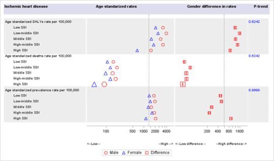
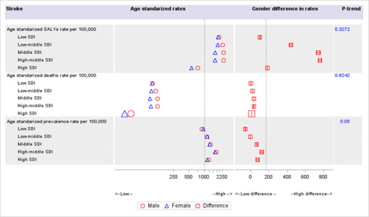
(C)    Stroke

Females had lower DALYs (per 100,000 population), deaths (per 100,000), and but higher prevalence (per 100,000) from stroke than males, and this gap remained unchanged across the SDI quintiles (p-trend >0.05). In the low SDI region, females witnessed 101 less DALYs from stroke (per 100,000 population) than males, which moderately increased to 185 DALYs per 100,000 in higher SDI regions. These findings suggest no evidence of a relationship between DALYs rate (per 100,000 population) and SDI quintiles. There was some evidence suggesting a relationship between SDI quintiles and gender-specific RHD prevalence rates (P-trend = 0.05).

I spent quite a bit of time exploring different visualization methods. I have always been fascinated by Gap minder's graphical presentation -- which I tried to re-create in SAS using graphic template language. It was a good learning experience.

Burden of cardiovascular disease from 1990-2017 by countries and region

These figures were created using graphic template language in SAS following a procedure developed by Robert (2019) (3). The GDP per capita (inflation-adjusted) are plotted in x-axis and corresponding values of gender difference in age-standardized cardiovascular disease (CVD) rates (male rates minus female rates) are plotted in y-axis. The size of bubble corresponds to the size of the population of the country. The definition of cardiovascular disease includes all eleven CVD types and is described elsewhere (4). The left map is for annotation and shows the world's region (America, East Asia & Pacific, Europe & Central Asia, Middle east & North Africa, South Asia, Sub-Saharan Africa). The data on cardiovascular disease rates were obtained from the Global Burden of Disease (4) and population data from World Bank (5). Sample codes are provided in supplementary appendix.

(A) Age-standardized DALYs rate of cardiovascular disease per 100,000 population from 1990 to 2017 by country's GDP/capita

(B) Age- standardized deaths rate of cardiovascular disease per 100,000 population from 1990 to 2017 by country's GDP/capita 

(C) Age- standardized prevalence rate of cardiovascular disease per 100,000 population on from 1990 to 2017 by country's GDP/capita  

Summary

 As the GDP goes up from 1990 to 2017, countries gradually shift from having higher CVD DALYs rates to lower CVD DALYs among women. Many countries were in the negative quadrant in 1990. These changes support our ealier findings that the gender difference has been continuously narrowing down for rheumatic heart disease and widening for stroke, across the SDI quintiles. 

Factors contributing to these shifts in CVD rates may include literary, income, and empowerment in women. Also, these changes should be interpreted in the context of existing data limitations. Further studies are needed to untangle the gendered impact of poverty in cardiovascular disease.

Supplementary appendix (click here)

References

1. O’Leary JR. How to Create a Journal Quality Forest Plot with SAS® 9.4. Available from https://www.pharmasug.org/proceedings/2017/QT/PharmaSUG-2017-QT15.pdf (accessed 7 May, 2020)

2. Park C, Hsiung JT, Soohoo M, Streja, E. Choosing Wisely: Using the Appropriate Statistical Test for Trend in SAS. Available from https://www.lexjansen.com/wuss/2019/175_Final_Paper_PDF.pdf (accessed 7 May 2020)

3. Robert A. Available from https://blogs.sas.com/content/sastraining/2019/01/24/re-creating-a-hans-rosling-graph-animation-with-sas/ (accessed 7 May 2020)

4. Global Burden of Disease Collaborative Network. Global Burden of Disease Study 2017 (GBD 2017) Results. Seattle, United States: Institute for Health Metrics and Evaluation (IHME), 2018. Available from. Available from http://ghdx.healthdata.org/gbd-results-tool (accessed 5 May 2020)

5. World Bank. Population Total. Available from http://wdi.worldbank.org/table/2.1# (accessed 5 May 2020)

[shivarajmishra]

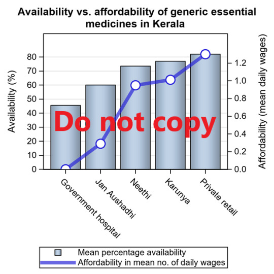
Journal Quality Barchart [+series overlay] using SGRENDER procedure in SAS/STAT 14.1, also SAS Studio

/**importing data set directly from sas studio enviornment**/ PROC SQL; CREATE TABLE WORK.query AS SELECT 'type'n , avail , afford , 'row'n FROM _TEMP5.coolviz1; RUN; QUIT;

PROC DATASETS NOLIST NODETAILS; CONTENTS DATA=WORK.query OUT=WORK.details; RUN;

PROC PRINT DATA=WORK.details; RUN;

/**creating dataset for vizualization**/ data data1; set  work.query;

if type = "Karunya" then delete; run;

proc freq data =data1;table type;run;

data myattrmap;  input id $ value $ markercolor $ markersymbol $; datalines; myid Cloudy grey cloud myid Sunny orange sun myid Showers blue umbrella ; run;

/**running the template procedure**/

proc template;  define statgraph Bar_line_2 ;    begingraph;      entrytitle 'Availability vs. affordability of generic essential medicines in Kerala';      layout overlay / xaxisopts=(display=(ticks tickvalues))                       yaxisopts=(griddisplay=on offsetmax=0.15 offsetmin=0 linearopts=                           (tickvaluesequence=(start=0 end=100 increment=5)))       y2axisopts=(offsetmin=0 offsetmax=0.15 linearopts=                           (tickvaluepriority=true tickvaluesequence=(start=0 end=1.2 increment=.2)));        barchart x=type y=avail / name='a' skin=modern legendlabel="Mean percentage availability" ;        barchart x=type y=afford /  yaxis=y2 datatransparency=1 ;        seriesplot x=type y=afford / yaxis=y2 name='b'                   lineattrs=graphdata1(thickness=5) datatransparency=0.3 legendlabel="Affordability in mean no. of daily wages" ;        scatterplot x=type y=afford / yaxis=y2                    markerattrs=graphdata1(symbol=circlefilled size=15);        scatterplot x=type y=afford / yaxis=y2                   markerattrs=(symbol=circlefilled size=11 color=white);

       discretelegend 'a' 'b' / location=outside valign=bottom halign=right across=1;      endlayout;    endgraph;  end; run;

/**running proc sgrender procedure**/

ods graphics / reset width=4in height=4.0in imagename='Bar_Line_GTL_2' noborder ; proc sgrender data=data1 template=Bar_line_2; run;

Where to get help?

1. Graphically speaking is a forum for SAS graph users, check out this website, https://blogs.sas.com/content/graphicallyspeaking/. I am a massive fan of Sanjay Matange. Make sure to check his graph templates:   https://blogs.sas.com/content/author/sanjaymatange/page/2/. I usually start with his set of codes and tweak and turn from there.

2. SAS community forum: check out what others have posted about your query

https://communities.sas.com/ 

[shivarajmishra]

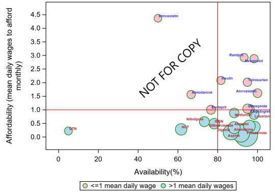
Bubble plot using SGPLOT  procedure in SAS/STAT 14.1

data pred; input type $1-16 avail afford  value ; format avail afford 4.0; label avail='Availability(%)'; label afford='Affordability (mean daily wages to afford monthly)'; row = _n_; datalines;

<<<set up your own data set>>> ; run;

data pred1; set pred; index=avail/afford;

 if value eq 1 then do; value1=">1 mean daily wages";end;  if value eq 2 then do; value1="<=1 mean daily wagess";end;

format value valuef.; run;

data attrmap;  id='A'; value='>1 mean daily wages'; fillcolor='lightblue'; textcolor='blue'; output;  id='A'; value='<=1 mean daily wagess'; fillcolor='pink'; textcolor='red'; output; run;

#modified SAS codes, based on a example from SAS forum#

%let dpi=300; ods listing gpath="C:\Extra inning" image_dpi=&dpi; ods graphics on/ reset width=5in height=4in noborder imagename='accessgraph'; proc sgplot data=pred1 dattrmap=attrmap; title "Availability and affordability of surveyed medicines in private sector";  bubble x=avail y=afford size=index/ group=value1 attrid=A lineattrs=(color=green)  name='a';  scatter x=avail y=afford / group=value datalabel=type datalabelattrs=(size=.05) markerattrs=(size=0)             datalabelattrs=(weight=bold) attrid=A; yaxis  min=0 values=(0 to 4.5 by .5);

refline 80 / axis=x lineattrs=(color=RED thickness=.05px pattern=solid); refline 1 / axis=y lineattrs=(color=RED thickness=.05px pattern=solid);  keylegend 'a' / location=outside position=bottom;  run;

[shivarajmishra]

DSW4: Machine Learning for Data Analysis (Python Programming)

Analysis: K-means cluster analysis

#Project: Demographic profiling of community health workers in Nepal #Dataset: fchv2014workingdata.csv, more info, link https://bit.ly/2T3fuV2

#loading the library first

import numpy import pandas import statsmodels.api as sm import seaborn import statsmodels.formula.api as smf

from pandas import Series, DataFrame import pandas as pd import numpy as np import os import matplotlib.pylab as plt from sklearn import tree from sklearn.model_selection import train_test_split from sklearn.tree import DecisionTreeClassifier from sklearn.metrics import classification_report from sklearn import preprocessing from sklearn.cluster import KMeans import sklearn.metrics

# Feature Importance

from sklearn import datasets from sklearn.ensemble import ExtraTreesClassifier

os.chdir("C:\Extra Innings\python")

#Load the dataset data = pd.read_csv("fchv2014workingdata.csv") data.dtypes data.describe()

# listwise deletion of missing values

sub1 = data[['age', 'literacy', 'Satis', 'q201', 'q203','hoursweekavg','residence',             'caste','q207','q209','q210','q301','q312num','q106','q309','q310']].dropna() sub1 = sub1.dropna() sub1.dtypes sub1.describe()

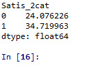
#lets split Satis into binary categorical variable def Satis_2cat (row):   if row['Satis'] >= 17 :      return 1   elif row['Satis'] < 17 :      return 0

sub1['Satis_2cat'] = sub1.apply (lambda row: Satis_2cat (row),axis=1)

c2= sub1.groupby('Satis_2cat').size()* 100 / len(data) print (c2)

#printing to see if it is dichotomized well

sub1=sub1[['Satis','Satis_2cat']] a = sub1.head (n=100) print(a)

#age

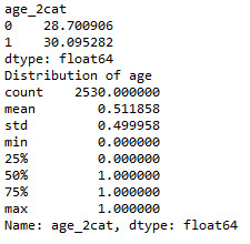
def age_2cat (row):  if row['q201'] >=38 :     return 1  elif row['q201'] <38 :     return 0

sub1['age_2cat'] = sub1.apply (lambda row: age_2cat (row),axis=1)

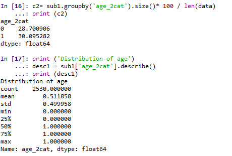
c2= sub1.groupby('age_2cat').size()* 100 / len(data) print (c2)

print ('Distribution of age') desc1 = sub1['age_2cat'].describe() print (desc1)

# education

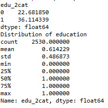
def edu_2cat (row):  if row['q203'] >= 7 :     return 1  elif row['q203'] < 7 :     return 0

sub1['edu_2cat'] = sub1.apply (lambda row: edu_2cat (row),axis=1)

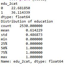
c2= sub1.groupby('edu_2cat').size()* 100 / len(data) print (c2)

print ('Distribution of education') desc1 = sub1['edu_2cat'].describe() print (desc1)

#hours worked per week

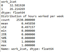
def work_2cat (row):  if row['hoursweekavg'] >= 8 :     return 1  elif row['hoursweekavg'] < 8 :     return 0

sub1['work_2cat'] = sub1.apply (lambda row: work_2cat (row),axis=1)

c2= sub1.groupby('work_2cat').size()* 100 / len(data) print (c2)

print ('Distribution of hours worked per week') desc1 = sub1['work_2cat'].describe() print (desc1)

#residence

print ('residence composition in the study sample') c2 = sub1['residence'].value_counts(sort=False) print (c2)

def score_to_numeric2(x):    if x=='urban':        return 1    if x=='rural':        return 0 sub1['residence'] = sub1['residence'].apply(score_to_numeric2) data

print ('residence composition in the study sample') c1 = sub1['residence'].value_counts(sort=False) print (c1)

#caste

print ('caste composition in the study sample') c1 = sub1['caste'].value_counts(sort=False) print (c1)

def score_to_numeric2(x):    if x=='others':        return 0    if x=='Hill caste':        return 1    if x=='Dalits':        return 0    if x=='Tarai/Madhesi castes':        return 0    if x=='Terai others':        return 0    if x=='Janajatis':        return 0    if x=='Muslim':        return 0 sub1['caste'] = sub1['caste'].apply(score_to_numeric2) data

print ('caste composition in the study sample') c1 = sub1['caste'].value_counts(sort=False) print (c1)

#’q207′ marital status

print ('marital status composition in the study sample') c2 = sub1['q207'].value_counts(sort=False) print (c2)

def score_to_numeric2(x):    if x=='currently married':        return 0    if x=='unmarried':        return 1    if x=='widow':        return 1    if x=='divorced/separated':        return 1

sub1['q207'] = sub1['q207'].apply(score_to_numeric2) data

print ('martial status composition in the study sample') c1 = sub1['q207'].value_counts(sort=False) print (c1)

print ('Distribution of years of work exp.') desc1 = sub1['q207'].describe() print (desc1)

#’q209′ family structure

print ('family structure composition in the study sample') c1 = sub1['q209'].value_counts(sort=False) print (c1)

def score_to_numeric2(x):    if x=='Extended Family':        return 1    if x=='Joint Family':        return 1    if x=='Nuclear Family':        return 0 sub1['q209'] = sub1['q209'].apply(score_to_numeric2) data

print ('family structure composition in the study sample') c1 = sub1['q209'].value_counts(sort=False) print (c1)

#’q210′ occupation

print ('occupational composition in the study sample') c1 = sub1['q210'].value_counts(sort=False) print (c1)

def score_to_numeric2(x):    if x=='teaching':        return 1    if x=='not involved in any other occupation':        return 0    if x=='petty business':        return 1    if x=='daily wage labour':        return 1    if x=='agriculture':        return 1    if x=='business':        return 1    if x=='others':        return 1    if x=='other services':        return 1

sub1['q210'] = sub1['q210'].apply(score_to_numeric2) data

print ('occupational composition in the study sample') c1 = sub1['q210'].value_counts(sort=False) print (c1)

#’q301′ years of work as chws

print ('Distribution of years of work exp.') desc1 = sub1['q301'].describe() print (desc1)

def exp_2cat (row):  if row['q301'] >= 14 :     return 1  elif row['q301'] < 14 :     return 0

sub1['exp_2cat'] = sub1.apply (lambda row: exp_2cat (row),axis=1)

c2= sub1.groupby('exp_2cat').size()* 100 / len(data) print (c2)

print ('Distribution of hours worked per week') desc1 = sub1['exp_2cat'].describe() print (desc1)

#’q312num’ time to reach health facility 

print ('time to reach health facility') desc1 = sub1['q312num'].describe() print (desc1)

def travel_2cat (row):  if row['q312num'] >= 30 :     return 1  elif row['q312num'] < 30 :     return 0

sub1['travel_2cat'] = sub1.apply (lambda row: travel_2cat (row),axis=1)

c2= sub1.groupby('travel_2cat').size()* 100 / len(data) print (c2)

print ('time to reach health facility') desc1 = sub1['travel_2cat'].describe() print (desc1)

#’q106′ numbers of houses in catchment

print ('numbers of houses in catchment') desc1 = sub1['q106'].describe() print (desc1)

def houses_2cat (row):  if row['q106'] >= 80 :     return 1  elif row['q106'] < 80 :     return 0

sub1['houses_2cat'] = sub1.apply (lambda row: houses_2cat (row),axis=1)

c2= sub1.groupby('houses_2cat').size()* 100 / len(data) print (c2)

print ('numbers of houses in catchmenty') desc1 = sub1['houses_2cat'].describe() print (desc1)

#’q309′ times of visit last month to health facility 

print ('times of visit last month to hf') desc1 = sub1['q309'].describe() print (desc1)

def visits_2cat (row):  if row['q309'] >= 2 :     return 1  elif row['q309'] < 2 :     return 0

sub1['visits_2cat'] = sub1.apply (lambda row: visits_2cat (row),axis=1)

c2= sub1.groupby('visits_2cat').size()* 100 / len(data) print (c2)

print ('times of visit last month to hf') desc1 = sub1['visits_2cat'].describe() print (desc1)

#’q310′ mode of transportation 

print ('transport options in the study sample') c1 = sub1['q310'].value_counts(sort=False) print (c1)

def score_to_numeric2(x):    if x=='others':        return 1    if x=='bus/keep/van':        return 1    if x=='cycle':        return 1    if x=='walking':        return 0    if x=='motorcycle':        return 1 sub1['transport_2cat'] = sub1['q310'].apply(score_to_numeric2)

print ('transport options in the study sample') c1 = sub1['transport_2cat'].value_counts(sort=False) print (c1)

#printing to see if it is dichotomized well

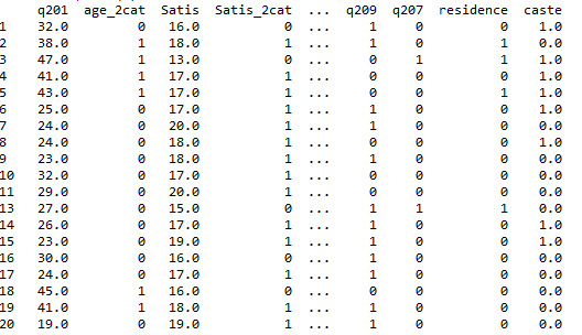
sub1=sub1[['q201','age_2cat','Satis','Satis_2cat','q203','edu_2cat','hoursweekavg','work_2cat','transport_2cat','visits_2cat','houses_2cat',           'travel_2cat','exp_2cat','exp_2cat','q210','q209','q207','residence','caste']] a = sub1.head (n=100) print(a)

#Modeling and Prediction #Split into training and testing sets

sub2 = sub1[['q201','age_2cat','Satis','Satis_2cat','q203','edu_2cat','hoursweekavg','work_2cat','transport_2cat','visits_2cat','houses_2cat',           'travel_2cat','exp_2cat','exp_2cat','q210','q209','q207','residence','caste']].dropna() cluster = sub2[['Satis', 'age_2cat','edu_2cat','work_2cat','transport_2cat','visits_2cat','houses_2cat',           'travel_2cat','exp_2cat','q210','q209','q207','residence','caste']] target =sub2.Satis_2cat

pred_train.shape pred_test.shape tar_train.shape tar_test.shape

#standarizing the cluster variable to have mean=0 and sd=1

clustervar=cluster.copy() from sklearn import preprocessing clustervar['age_2cat']=preprocessing.scale(clustervar['age_2cat'].astype('float64')) clustervar['edu_2cat']=preprocessing.scale(clustervar['edu_2cat'].astype('float64')) clustervar['work_2cat']=preprocessing.scale(clustervar['work_2cat'].astype('float64')) clustervar['transport_2cat']=preprocessing.scale(clustervar['transport_2cat'].astype('float64')) clustervar['visits_2cat']=preprocessing.scale(clustervar['visits_2cat'].astype('float64')) clustervar['houses_2cat']=preprocessing.scale(clustervar['houses_2cat'].astype('float64')) clustervar['travel_2cat']=preprocessing.scale(clustervar['travel_2cat'].astype('float64')) clustervar['exp_2cat']=preprocessing.scale(clustervar['exp_2cat'].astype('float64')) clustervar['q210']=preprocessing.scale(clustervar['q210'].astype('float64')) clustervar['q209']=preprocessing.scale(clustervar['q209'].astype('float64')) clustervar['q207']=preprocessing.scale(clustervar['q207'].astype('float64')) clustervar['residence']=preprocessing.scale(clustervar['residence'].astype('float64')) clustervar['caste']=preprocessing.scale(clustervar['caste'].astype('float64'))

# split data into train and test sets

clus_train, clus_test = train_test_split(clustervar, test_size=.3, random_state=123)

# k-means cluster analysis for 1-9 clusters                                        

from scipy.spatial.distance import cdist clusters=range(1,10) meandist=[]

for k in clusters:    model=KMeans(n_clusters=k)    model.fit(clus_train)    clusassign=model.predict(clus_train)    meandist.append(sum(np.min(cdist(clus_train, model.cluster_centers_, 'euclidean'), axis=1))    / clus_train.shape[0])

# The syntax below plots the average distance of observations from cluster-centroid by using the Elbow Method 

plt.plot(clusters, meandist) plt.xlabel('Number of clusters') plt.ylabel('Average distance') plt.title('Selecting k with the Elbow Method')

# Interpret 3 cluster solution

model3=KMeans(n_clusters=3) model3.fit(clus_train) clusassign=model3.predict(clus_train)

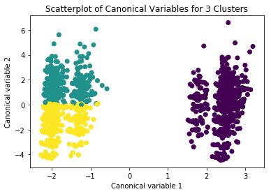
# plot clusters

from sklearn.decomposition import PCA pca_2 = PCA(2) plot_columns = pca_2.fit_transform(clus_train) plt.scatter(x=plot_columns[:,0], y=plot_columns[:,1], c=model3.labels_,) plt.xlabel('Canonical variable 1') plt.ylabel('Canonical variable 2') plt.title('Scatterplot of Canonical Variables for 3 Clusters') plt.show()

#BEGIN multiple steps to merge cluster assignment with clustering variables to examine cluster variable means by cluster

# create a unique identifier variable from the index for the cluster training data to merge with the cluster assignment variable

clus_train.reset_index(level=0, inplace=True)

# create a list that has the new index variable

cluslist=list(clus_train['index'])

# create a list of cluster assignments

labels=list(model3.labels_) # combine index variable list with cluster assignment list into a dictionary newlist=dict(zip(cluslist, labels)) newlist

# convert newlist dictionary to a dataframe

newclus=DataFrame.from_dict(newlist, orient='index') newclus # rename the cluster assignment column newclus.columns = ['cluster']

# now do the same for the cluster assignment variable # create a unique identifier variable from the index for the cluster assignment dataframe  to merge with cluster training data

newclus.reset_index(level=0, inplace=True)

# merge the cluster assignment dataframe with the cluster training variable dataframe # by the index variable

merged_train=pd.merge(clus_train, newclus, on='index') merged_train.head(n=100) # cluster frequencies merged_train.cluster.value_counts()

#END multiple steps to merge cluster assignment with clustering variables to examine cluster variable means by cluster

# FINALLY calculate clustering variable means by cluster

clustergrp = merged_train.groupby('cluster').mean() print ("Clustering variable means by cluster") print(clustergrp)

# validate clusters in training data by examining cluster differences in Satis using ANOVA # first have to merge Satis with clustering variables and cluster assignment data

Satis_data=sub1['Satis'] # split Satis data into train and test sets Satis_train, Satis_test = train_test_split(Satis_data, test_size=.3, random_state=123) Satis_train1=pd.DataFrame(Satis_train) Satis_train1.reset_index(level=0, inplace=True) merged_train_all=pd.merge(Satis_train1, merged_train, on='index') sub1 = merged_train_all[['Satis', 'cluster']].dropna()

import statsmodels.formula.api as smf import statsmodels.stats.multicomp as multi

gpamod = smf.ols(formula='Satis ~ C(cluster)', data=sub1).fit() print (gpamod.summary())

print ('means for Satis by cluster') m1= sub1.groupby('cluster').mean() print (m1)

print ('standard deviations for Satis by cluster') m2= sub1.groupby('cluster').std() print (m2)

mc1 = multi.MultiComparison(sub1['Satis'], sub1['cluster']) res1 = mc1.tukeyhsd() print(res1.summary())

Interpretations 

Our model has thirteen variables: age, education, caste, residence, martial status, family structure, occupation, hours worked per week, years of experience as CHWs, traveling time to reach health facility, number of houses in catchment area, number visits to health facility, and mode of transportation. The variables has been defined in previous assignment (link,https://bit.ly/2UlVCx2) .The size ratio was set at 60% for training sample and 40% for test sample. A total of 3 clusters were built using the k-means cluster analysis technique. The Elbow method showed that with additional clusters added into the model the average distance from the centroid decreased. 

The overall accuracy of clusters based on canonical variable was reasonable without much overlap between any clusters i.e. model correctly specified reduced the thirteen variables into 3 clusters. We also calculated the mean and standard deviation of ‘satisfaction score’ across this newly created cluster variable.The mean satisfaction was higher in cluster 2 (Mean: 18.1) followed by cluster 1 (Mean: 16.9) and cluster 0 (Mean: 15.6). The ANOVA test of means showed that these means were actually different across this newly created variable (F=5.4, p=0.004). The post-hoc tests show the differences between cluster 0 and cluster 1 followed by the difference between cluster 1 and 2 are statistically significant. 

[shivarajmishra]

DSW3. Machine Learning for Data Analysis (Python Programming)

#Analysis: Lasso regression 

#Project: Demographic profiling of community health workers in Nepal #Dataset: fchv2014workingdata.csv, more info, link https://bit.ly/2T3fuV2

#loading the library first

#week3-machine learning import numpy import pandas import statsmodels.api as sm import seaborn import statsmodels.formula.api as smf

from pandas import Series, DataFrame import pandas as pd import numpy as np import os import matplotlib.pylab as plt from sklearn import tree from sklearn.model_selection import train_test_split from sklearn.tree import DecisionTreeClassifier from sklearn.metrics import classification_report from sklearn.linear_model import LassoLarsCV import sklearn.metrics

# Feature Importance from sklearn import datasets from sklearn.ensemble import ExtraTreesClassifier

os.chdir("C:\Extra Innings\python")

#Load the dataset

data = pd.read_csv("fchv2014workingdata.csv") data.dtypes data.describe()

# listwise deletion of missing values sub1 = data[['age', 'literacy', 'Satis', 'q201', 'q203','hoursweekavg','residence',             'caste','q207','q209','q210','q301','q312num','q106','q309','q310']].dropna() sub1 = sub1.dropna()

sub1.dtypes sub1.describe()

#lets split Satis into binary categorical variable

def Satis_2cat (row):   if row['Satis'] >= 17 :      return 1   elif row['Satis'] < 17 :      return 0

sub1['Satis_2cat'] = sub1.apply (lambda row: Satis_2cat (row),axis=1)

c2= sub1.groupby('Satis_2cat').size()* 100 / len(data) print (c2)

#printing to see if it is dichotomized well sub1=sub1[['Satis','Satis_2cat']] a = sub1.head (n=100) print(a)

#age

def age_2cat (row):  if row['q201'] >=38 :     return 1  elif row['q201'] <38 :     return 0

sub1['age_2cat'] = sub1.apply (lambda row: age_2cat (row),axis=1)

c2= sub1.groupby('age_2cat').size()* 100 / len(data) print (c2)

print ('Distribution of age') desc1 = sub1['age_2cat'].describe() print (desc1)

# education

def edu_2cat (row):  if row['q203'] >= 7 :     return 1  elif row['q203'] < 7 :     return 0

sub1['edu_2cat'] = sub1.apply (lambda row: edu_2cat (row),axis=1)

c2= sub1.groupby('edu_2cat').size()* 100 / len(data) print (c2)

print ('Distribution of education') desc1 = sub1['edu_2cat'].describe() print (desc1)

#hours worked per week

def work_2cat (row):  if row['hoursweekavg'] >= 8 :     return 1  elif row['hoursweekavg'] < 8 :     return 0

sub1['work_2cat'] = sub1.apply (lambda row: work_2cat (row),axis=1)

c2= sub1.groupby('work_2cat').size()* 100 / len(data) print (c2)

print ('Distribution of hours worked per week') desc1 = sub1['work_2cat'].describe() print (desc1)

#residence

print ('residence composition in the study sample') c2 = sub1['residence'].value_counts(sort=False) print (c2)

def score_to_numeric2(x):    if x=='urban':        return 1    if x=='rural':        return 0 sub1['residence'] = sub1['residence'].apply(score_to_numeric2) data

print ('residence composition in the study sample') c1 = sub1['residence'].value_counts(sort=False) print (c1)

#caste

print ('caste composition in the study sample') c1 = sub1['caste'].value_counts(sort=False) print (c1)

def score_to_numeric2(x):    if x=='others':        return 0    if x=='Hill caste':        return 1    if x=='Dalits':        return 0    if x=='Tarai/Madhesi castes':        return 0    if x=='Terai others':        return 0    if x=='Janajatis':        return 0    if x=='Muslim':        return 0 sub1['caste'] = sub1['caste'].apply(score_to_numeric2) data

print ('caste composition in the study sample') c1 = sub1['caste'].value_counts(sort=False) print (c1)

#’q207′ marital status

print ('marital status composition in the study sample') c2 = sub1['q207'].value_counts(sort=False) print (c2)

def score_to_numeric2(x):    if x=='currently married':        return 0    if x=='unmarried':        return 1    if x=='widow':        return 1    if x=='divorced/separated':        return 1

sub1['q207'] = sub1['q207'].apply(score_to_numeric2) data

print ('martial status composition in the study sample') c1 = sub1['q207'].value_counts(sort=False) print (c1)

print ('Distribution of years of work exp.') desc1 = sub1['q207'].describe() print (desc1)

#’q209′ family structure

print ('family structure composition in the study sample') c1 = sub1['q209'].value_counts(sort=False) print (c1)

def score_to_numeric2(x):    if x=='Extended Family':        return 1    if x=='Joint Family':        return 1    if x=='Nuclear Family':        return 0 sub1['q209'] = sub1['q209'].apply(score_to_numeric2) data

print ('family structure composition in the study sample') c1 = sub1['q209'].value_counts(sort=False) print (c1)

#’q210′ occupation

print ('occupational composition in the study sample') c1 = sub1['q210'].value_counts(sort=False) print (c1)

def score_to_numeric2(x):    if x=='teaching':        return 1    if x=='not involved in any other occupation':        return 0    if x=='petty business':        return 1    if x=='daily wage labour':        return 1    if x=='agriculture':        return 1    if x=='business':        return 1    if x=='others':        return 1    if x=='other services':        return 1

sub1['q210'] = sub1['q210'].apply(score_to_numeric2) data

print ('occupational composition in the study sample') c1 = sub1['q210'].value_counts(sort=False) print (c1)

#’q301′ years of work as chws

print ('Distribution of years of work exp.') desc1 = sub1['q301'].describe() print (desc1)

def exp_2cat (row):  if row['q301'] >= 14 :     return 1  elif row['q301'] < 14 :     return 0

sub1['exp_2cat'] = sub1.apply (lambda row: exp_2cat (row),axis=1)

c2= sub1.groupby('exp_2cat').size()* 100 / len(data) print (c2)

print ('Distribution of hours worked per week') desc1 = sub1['exp_2cat'].describe() print (desc1)

#’q312′ num time to reach health facility 

print ('time to reach health facility') desc1 = sub1['q312num'].describe() print (desc1)

def travel_2cat (row):  if row['q312num'] >= 30 :     return 1  elif row['q312num'] < 30 :     return 0

sub1['travel_2cat'] = sub1.apply (lambda row: travel_2cat (row),axis=1)

c2= sub1.groupby('travel_2cat').size()* 100 / len(data) print (c2)

print ('time to reach health facility') desc1 = sub1['travel_2cat'].describe() print (desc1)

#’q106′ numbers of houses in catchment

print ('numbers of houses in catchment') desc1 = sub1['q106'].describe() print (desc1)

def houses_2cat (row):  if row['q106'] >= 80 :     return 1  elif row['q106'] < 80 :     return 0

sub1['houses_2cat'] = sub1.apply (lambda row: houses_2cat (row),axis=1)

c2= sub1.groupby('houses_2cat').size()* 100 / len(data) print (c2)

print ('numbers of houses in catchmenty') desc1 = sub1['houses_2cat'].describe() print (desc1)

#’q309′ number of times of visit last month to health facility

print ('times of visit last month to hf') desc1 = sub1['q309'].describe() print (desc1)

def visits_2cat (row):  if row['q309'] >= 2 :     return 1  elif row['q309'] < 2 :     return 0

sub1['visits_2cat'] = sub1.apply (lambda row: visits_2cat (row),axis=1)

c2= sub1.groupby('visits_2cat').size()* 100 / len(data) print (c2)

print ('times of visit last month to hf') desc1 = sub1['visits_2cat'].describe() print (desc1)

#’q310′ mode of transportation 

print ('transport options in the study sample') c1 = sub1['q310'].value_counts(sort=False) print (c1)

def score_to_numeric2(x):    if x=='others':        return 1    if x=='bus/keep/van':        return 1    if x=='cycle':        return 1    if x=='walking':        return 0    if x=='motorcycle':        return 1 sub1['transport_2cat'] = sub1['q310'].apply(score_to_numeric2)

print ('transport options in the study sample') c1 = sub1['transport_2cat'].value_counts(sort=False) print (c1)

#printing to see if it is dichotomized well

sub1=sub1[['q201','age_2cat','Satis','Satis_2cat','q203','edu_2cat','hoursweekavg','work_2cat','transport_2cat','visits_2cat','houses_2cat',           'travel_2cat','exp_2cat','exp_2cat','q210','q209','q207','residence','caste']] a = sub1.head (n=100) print(a)

#Modeling and Prediction

#Split into training and testing sets

sub2 = sub1[['q201','age_2cat','Satis','Satis_2cat','q203','edu_2cat','hoursweekavg','work_2cat','transport_2cat','visits_2cat','houses_2cat',           'travel_2cat','exp_2cat','exp_2cat','q210','q209','q207','residence','caste']].dropna() predvar = sub2[['age_2cat','edu_2cat','work_2cat','transport_2cat','visits_2cat','houses_2cat',           'travel_2cat','exp_2cat','q210','q209','q207','residence','caste']] target =sub2.Satis_2cat

pred_train.shape pred_test.shape tar_train.shape tar_test.shape

# standardize predictors to have mean=0 and sd=1

predictors=predvar.copy() from sklearn import preprocessing predictors['age_2cat']=preprocessing.scale(predictors['age_2cat'].astype('float64')) predictors['edu_2cat']=preprocessing.scale(predictors['edu_2cat'].astype('float64')) predictors['work_2cat']=preprocessing.scale(predictors['work_2cat'].astype('float64')) predictors['transport_2cat']=preprocessing.scale(predictors['transport_2cat'].astype('float64')) predictors['visits_2cat']=preprocessing.scale(predictors['visits_2cat'].astype('float64')) predictors['houses_2cat']=preprocessing.scale(predictors['houses_2cat'].astype('float64')) predictors['travel_2cat']=preprocessing.scale(predictors['travel_2cat'].astype('float64')) predictors['exp_2cat']=preprocessing.scale(predictors['exp_2cat'].astype('float64')) predictors['q210']=preprocessing.scale(predictors['q210'].astype('float64')) predictors['q209']=preprocessing.scale(predictors['q209'].astype('float64')) predictors['q207']=preprocessing.scale(predictors['q207'].astype('float64')) predictors['residence']=preprocessing.scale(predictors['residence'].astype('float64')) predictors['caste']=preprocessing.scale(predictors['caste'].astype('float64'))

# split data into train and test sets

pred_train, pred_test, tar_train, tar_test = train_test_split(predictors, target,                                                              test_size=.3, random_state=123) # specify the lasso regression model model=LassoLarsCV(cv=10, precompute=False).fit(pred_train,tar_train)

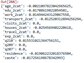
# print variable names and regression coefficients dict(zip(predictors.columns, model.coef_))

# plot coefficient progression

m_log_alphas = -np.log10(model.alphas_) ax = plt.gca() plt.plot(m_log_alphas, model.coef_path_.T) plt.axvline(-np.log10(model.alpha_), linestyle='--', color='k',            label='alpha CV') plt.ylabel('Regression Coefficients') plt.xlabel('-log(alpha)') plt.title('Regression Coefficients Progression for Lasso Paths')

# plot mean square error for each folds

m_log_alphascv = -np.log10(model.cv_alphas_) plt.figure() plt.plot(m_log_alphascv, model.mse_path_, ':') plt.plot(m_log_alphascv, model.mse_path_.mean(axis=-1), 'k',         label='Average across the folds', linewidth=2) plt.axvline(-np.log10(model.alpha_), linestyle='--', color='k',            label='alpha CV') plt.legend() plt.xlabel('-log(alpha)') plt.ylabel('Mean squared error') plt.title('Mean squared error on each fold')

# MSE from training and test data

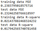
from sklearn.metrics import mean_squared_error train_error = mean_squared_error(tar_train, model.predict(pred_train)) test_error = mean_squared_error(tar_test, model.predict(pred_test)) print ('training data MSE') print(train_error) print ('test data MSE') print(test_error)

# R-square from training and test data

rsquared_train=model.score(pred_train,tar_train) rsquared_test=model.score(pred_test,tar_test) print ('training data R-square') print(rsquared_train) print ('test data R-square') print(rsquared_test)

Interpretations

Our model has thirteen predictor/explanatory variables: age, education, caste, residence, martial status, family structure, occupation, hours worked per week, years of experience as CHWs, traveling time to reach health facility, number of houses in catchment area, number visits to health facility, and mode of transportation. These variables has been defined in previous assignment (link,https://bit.ly/2UlVCx2).The outcome variable ‘satisfaction score is a binary variable (>=17, <17). For lasso regression, the size ratio was set at 60% for the training sample and 40% for the test sample. 

Predictors with a regression coefficient which do not have a value of zero are included in the lasso regression model. Predictors with a regression coefficient equal to zero means that the variables have shrunk to zero after applying lasso regression penalty terms and subsequently removed from the model. Out of the thirteen variables, eight with non-zero coefficient were selected into the model. Based on the value of regression coefficient we can say that those CHWs which live in an area with more than 80 houses in the catchment have 0.025 times lower chances of having >=17 satisfaction score. Those who walk to the health facility had the weakest association with satisfaction score: those who travel by bus/transportation options had 0.013 times lower chances of having >=17 satisfaction score.

We also plotted the regression coefficients for lasso paths, and similarly, the mean square errors in each fold were plotted. The lasso paths showed the relative importance of predictor variables selected at any stage of selection process i.e. how regression coefficients change with the addition of new variables at each step. ‘CHWs catchment area’ had the largest regression coefficient, therefore, it was entered into the model first, and this was followed by ‘age’. The final variable entered into the model was ‘means of transportation’. The mean square errors plot showed a degree of variability across the individual cross-validation folds in the training data set. However, the changes in the mean square error followed the same pattern for each fold as variables were added to the model. It decreased at the beginning and then levelled off at a point where adding extra variables did not lead to much reduction in mean square errors. 

The selected model was less accurate in predicting satisfaction score. However, the test and training mean square errors were not much different. Training dataset explained nearly 2.1% of the variance in the data compared to 1.8% by test data.

[shivarajmishra]

DSW2. Machine Learning for Data Analysis (Python Programming)

#Project: Demographic profiling of community health workers in Nepal #Dataset: fchv2014workingdata.csv, more info, link https://bit.ly/2T3fuV2

#loading the library first 

pip help import numpy import pandas import statsmodels.api as sm import seaborn import statsmodels.formula.api as smf

from pandas import Series, DataFrame import pandas as pd import numpy as np import os import matplotlib.pylab as plt from sklearn import tree from sklearn.model_selection import train_test_split from sklearn.tree import DecisionTreeClassifier from sklearn.metrics import classification_report import sklearn.metrics

# Feature Importance

from sklearn import datasets from sklearn.ensemble import ExtraTreesClassifier

os.chdir("C:\Extra Innings\python")

#Load the dataset

data = pd.read_csv("fchv2014workingdata.csv") data.dtypes data.describe()

# convert to numeric format

data['Satis'] = pandas.to_numeric(data['Satis'], errors='coerce') data['q201'] = pandas.to_numeric(data['q201'], errors='coerce') data['q203'] = pandas.to_numeric(data['q203'], errors='coerce') data['hoursweekavg'] = pandas.to_numeric(data['hoursweekavg'], errors='coerce')

# list-wise deletion of missing values

sub1 = data[['age', 'literacy', 'Satis', 'q201', 'q203','hoursweekavg']].dropna() sub1 = sub1.dropna()

sub1.dtypes sub1.describe()

#lets split Satis into binary categorical variable

def Satis_2cat (row):   if row['Satis'] >= 17 :      return 1   elif row['Satis'] < 17 :      return 0

sub1['Satis_2cat'] = sub1.apply (lambda row: Satis_2cat (row),axis=1)

c2= sub1.groupby('Satis_2cat').size()* 100 / len(data) print (c2)

#printing to see if it is dichotomized well

sub1=sub1[['Satis','Satis_2cat']] a = sub1.head (n=100) print(a)

#age

def age_2cat (row):  if row['q201'] >= 38 :     return 1  elif row['q201'] < 38 :     return 0

sub1['age_2cat'] = sub1.apply (lambda row: age_2cat (row),axis=1)

c2= sub1.groupby('age_2cat').size()* 100 / len(data) print (c2)

print ('Distribution of age') desc1 = sub1['age_2cat'].describe() print (desc1)

# education

def edu_2cat (row):  if row['q203'] >= 7 :     return 1  elif row['q203'] < 7 :     return 0

sub1['edu_2cat'] = sub1.apply (lambda row: edu_2cat (row),axis=1)

c2= sub1.groupby('edu_2cat').size()* 100 / len(data) print (c2)

print ('Distribution of education') desc1 = sub1['edu_2cat'].describe() print (desc1)

#hours worked per week

def work_2cat (row):  if row['hoursweekavg'] >= 8 :     return 1  elif row['hoursweekavg'] < 8 :     return 0

sub1['work_2cat'] = sub1.apply (lambda row: work_2cat (row),axis=1)

c2= sub1.groupby('work_2cat').size()* 100 / len(data) print (c2)

print ('Distribution of hours worked per week') desc1 = sub1['work_2cat'].describe() print (desc1)

#printing to see if it is dichotomized well

sub1=sub1[['q201','age_2cat','Satis','Satis_2cat','q203','edu_2cat','hoursweekavg','work_2cat']] a = sub1.head (n=100) print(a)

#Modeling and prediction

#Split into training and testing sets sub2 = sub1[['Satis_2cat', 'age_2cat','edu_2cat','work_2cat']].dropna() predictors = sub2[['age_2cat','edu_2cat','work_2cat']] targets =sub2.Satis_2cat pred_train, pred_test, tar_train, tar_test  =   train_test_split(predictors, targets, test_size=.4)

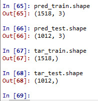
pred_train.shape pred_test.shape tar_train.shape tar_test.shape

#Build model on training data

from sklearn.ensemble import RandomForestClassifier

classifier=RandomForestClassifier(n_estimators=25) classifier=classifier.fit(pred_train,tar_train)

predictions=classifier.predict(pred_test)

sklearn.metrics.confusion_matrix(tar_test,predictions) sklearn.metrics.accuracy_score(tar_test, predictions)

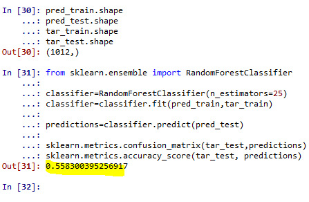
#note that overall accuracy for the Forrest plot is 0.56 which means that nearly 56% pf sample is correctly categorized as having >=17 or <17 satisfaction score.

# fit an Extra Trees model to the data

model = ExtraTreesClassifier()

model.fit(pred_train,tar_train)

# display the relative importance of each attribute

print(model.feature_importances_)

trees=range(25) accuracy=np.zeros(25)

for idx in range(len(trees)):   classifier=RandomForestClassifier(n_estimators=idx + 1)   classifier=classifier.fit(pred_train,tar_train)   predictions=classifier.predict(pred_test)   accuracy[idx]=sklearn.metrics.accuracy_score(tar_test, predictions)

plt.cla() plt.plot(trees, accuracy)

#with the first tree the accuracy is nearly 56% and remained constant  with addition of successive trees.

#Interpretation

#Our model has age, education and hours worked per week as the predictor/explanatory variable and satisfaction score (statis_2cat) as target variable. The size ratio was set at 60% for training sample and 40% for test sample. A total of 25 trees were built using the algorithm. The overall accuracy for the Forrest plot is 56% i.e. model correctly specified nearly 56% of sample into either low (<17) or high (>=17) satisfaction category. We also listed the variable based on their relative importance and found that education is more important than either age (0.30) and number of hours worked per week (0.16). Finally, based on the trees grown out of the Forrest plot we found that it is perfectly fine to interpret the results based on just single tree.

[shivarajmishra]

DSW1. Machine Learning for Data Analysis (Python Programming)

#Project: Demographic profiling of community health workers in Nepal

#Dataset: fchv2014workingdata.csv, more info, link https://bit.ly/2T3fuV2

#loading the library first

from pandas import Series, DataFrame import pandas as pd import numpy as np import os import matplotlib.pylab as plt from sklearn.cross_validation import train_test_split from sklearn.tree import DecisionTreeClassifier from sklearn.metrics import classification_report import sklearn.metrics

os.chdir("C:\Extra Innings\python")

Data Engineering and Analysis #Load the dataset

CHW_data = pd.read_csv("fchv2014workingdata.csv") data_clean = CHW_data.dropna()

data_clean.dtypes data_clean.describe()

# convert to numeric format

data['Satis'] = pandas.to_numeric(data['Satis'], errors='coerce') data['q201'] = pandas.to_numeric(data['q201'], errors='coerce') data['q203'] = pandas.to_numeric(data['q203'], errors='coerce') data['hoursweekavg'] = pandas.to_numeric(data['hoursweekavg'], errors='coerce')

# list-wise deletion of missing values

sub1 = data[['age', 'literacy', 'Satis', 'q201', 'q203','hoursweekavg']].dropna()

#lets split Satis into binary categorical variable #satisfaction score def Satis_2cat (row):   if row['Satis'] >= 17 :      return 1   elif row['Satis'] < 17 :      return 0

sub1['Satis_2cat'] = sub1.apply (lambda row: Satis_2cat (row),axis=1)

c2= sub1.groupby('Satis_2cat').size()* 100 / len(data) print (c2)

#age

def age_2cat (row):   if row['q201'] >= 38 :      return 1   elif row['q201'] < 38 :      return 0

sub1['age_2cat'] = sub1.apply (lambda row: age_2cat (row),axis=1)

c2= sub1.groupby('age_2cat').size()* 100 / len(data) print (c2)

print ('Distribution of age') desc1 = sub1['age_2cat'].describe() print (desc1)

# education

def edu_2cat (row):   if row['q203'] >= 7 :      return 1   elif row['q203'] < 7 :      return 0

sub1['edu_2cat'] = sub1.apply (lambda row: edu_2cat (row),axis=1)

c2= sub1.groupby('edu_2cat').size()* 100 / len(data) print (c2)

print ('Distribution of education') desc1 = sub1['edu_2cat'].describe() print (desc1)

#hours worked per week

def work_2cat (row):   if row['hoursweekavg'] >= 8 :      return 1   elif row['hoursweekavg'] < 8 :      return 0

sub1['work_2cat'] = sub1.apply (lambda row: work_2cat (row),axis=1)

c2= sub1.groupby('work_2cat').size()* 100 / len(data) print (c2)

print ('Distribution of hours worked per week') desc1 = sub1['work_2cat'].describe() print (desc1)

#printing to see if it is dichotomized well sub1=sub1[['q201','age_2cat','Satis', 'Satis_2cat', 'q203','edu_2cat','hoursweekavg','work_2cat']] a = sub1.head (n=100) print(a)

#Modeling and Prediction

#Split into training and testing sets sub2 = sub1[['Satis_2cat', 'age_2cat','edu_2cat','work_2cat']].dropna()

predictors = sub2[['age_2cat','edu_2cat','work_2cat']]

targets =sub2.Satis_2cat

pred_train, pred_test, tar_train, tar_test  =   train_test_split(predictors, targets, test_size=.4)

pred_train.shape pred_test.shape tar_train.shape tar_test.shape

#Build model on training data

classifier=DecisionTreeClassifier() classifier=classifier.fit(pred_train,tar_train)

predictions=classifier.predict(pred_test)

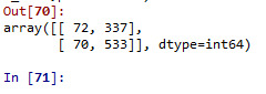
sklearn.metrics.confusion_matrix(tar_test,predictions) sklearn.metrics.accuracy_score(tar_test, predictions)

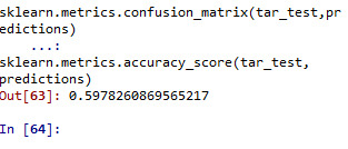
#which suggest that the model has correctly specified nearly 60% of sample correctly into either low (<17) or high (>=17) statisfaction score

#Displaying the decision tree

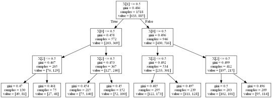
from sklearn import tree #from StringIO import StringIO from io import StringIO #from StringIO import StringIO from IPython.display import Image out = StringIO() tree.export_graphviz(classifier, out_file=out) import pydotplus graph=pydotplus.graph_from_dot_data(out.getvalue()) Image(graph.create_png())

Interpretation

Our model has age, education and hours worked per week as the predictor/explanatory variable and satisfaction score (statis_2cat) as target variable. The resulting tree starts with split on x0 that is education less than or equal to seven years of education. If the education has a value 0.5 that is education less than 7 years of education, the tree moves to the left side, including 572 observation in training sample. Other splits are made at education at second and hours worked per week at third node.Those with education <7 years of education, aged <38 years and worked <8 years per week classified 130 into this category: among which 49 had satisfaction score <17 and 81 had satisfaction score >=17.

Following on the right hand side of the tree, among those with education <7 years of education, aged <38 years and worked >=8 years per week classified 75 into this category: among which 27 had satisfaction score <17 and 48 had satisfaction score >=17.

Following that on the extreme right side of the tree, the two terminal leaves tell us those who have education >=7 years of education, aged >=38 years and worked >=8 years per week classified 209 into this category: among which 95 had satisfaction score <17 and 114 had satisfaction score >=17.

The model  correctly specified nearly 60% of sample correctly into either low (<17) or high (>=17) satisfaction category.

[shivarajmishra]

DSW4. Regression modeling in practice (Python Programming)

#Project: Demographic profiling of community health workers in Nepal

#Dataset: fchv2014workingdata.csv, more info, link https://bit.ly/2T3fuV2

#loading the library first

import numpy import pandas import statsmodels.api as sm import seaborn import statsmodels.formula.api as smf

# bug fix for display formats to avoid run time errors

pandas.set_option('display.float_format', lambda x:'%.2f'%x)

data = pandas.read_csv('fchv2014workingdata.csv', low_memory=False)

# convert to numeric format data['Satis'] = pandas.to_numeric(data['Satis'], errors='coerce') data['q201'] = pandas.to_numeric(data['q201'], errors='coerce') data['q203'] = pandas.to_numeric(data['q203'], errors='coerce') data['hoursweekavg'] = pandas.to_numeric(data['hoursweekavg'], errors='coerce')

# listwise deletion of missing values

sub1 = data[['age', 'literacy', 'Satis', 'q201', 'q203','hoursweekavg']].dropna()

#lets split Satis into binary categorical variable

def Satis_2cat (row):   if row['Satis'] >= 17 :      return 1   elif row['Satis'] < 17 :      return 0

sub1['Satis_2cat'] = sub1.apply (lambda row: Satis_2cat (row),axis=1)

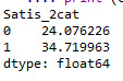
c2= sub1.groupby('Satis_2cat').size()* 100 / len(data) print (c2)

#printing to see if it is dichotomized well

sub1=sub1[['Satis', 'Satis_2cat']] a = sub1.head (n=100) print(a)

# center quantitative IVs for regression analysis

sub1['q201_c'] = (data['q201'] - data['q201'].mean()) sub1['hoursweekavg_c'] = (data['hoursweekavg'] - data['hoursweekavg'].mean()) sub1['q203_c'] = (data['q203'] - data['q203'].mean()) sub1[["q201_c", "hoursweekavg_c", "q203_c"]].describe()

# logistic regression with age (years) only into the model

lreg1 = smf.logit(formula = 'Satis_2cat ~ q201_c', data = sub1).fit() print (lreg1.summary()) # odds ratios print ("Odds Ratios") print (numpy.exp(lreg1.params))

# odd ratios with 95% confidence intervals

params = lreg1.params conf = lreg1.conf_int() conf['OR'] = params conf.columns = ['Lower CI', 'Upper CI', 'OR'] print (numpy.exp(conf))

# logistic regression with age and education 

lreg2 = smf.logit(formula = 'Satis_2cat ~ q201_c + q203_c', data = sub1).fit() print (lreg2.summary())

# odd ratios with 95% confidence intervals

params = lreg2.params conf = lreg2.conf_int() conf['OR'] = params conf.columns = ['Lower CI', 'Upper CI', 'OR'] print (numpy.exp(conf))

# logistic regression with age, education and hours worked per week

lreg3 = smf.logit(formula = 'Satis_2cat ~ q201_c + q203_c+ hoursweekavg_c', data = sub1).fit() print (lreg3.summary())

# odd ratios with 95% confidence intervals

print ("Odds Ratios") params = lreg3.params conf = lreg3.conf_int() conf['OR'] = params conf.columns = ['Lower CI', 'Upper CI', 'OR'] print (numpy.exp(conf))

Interpretation

In this analyses, a logistic regression modeling of binary satisfaction score variable (>=17,<17) and explanatory variable was performed. We build three logistic regression models, with 1) age, 2) age and education, 3) age, education and hours worked per week.

The first model showed that one year increment in age was associated with 0.99 (95%CI: 0.99, 1.00) times higher odds of having >=17 satisfaction score. In the second model which was further adjusted for education, the effect estimates for age remained unchanged. The association between education and satisfaction score >=17 however was statistically significant (OR=0.92, 95%CI: 0.90,0.95). Which means that each additional year of completed education is associated with 10% reduction in satisfaction score of >=17. The final model which further included hours worked per week, did not affect the earlier estimates. The hours worked per week was not statistically associated with satisfaction score of >=17 (OR=1.01, 95%CI: 0.99, 1.02).

There was no evidence of confounding effect on either of the association of age, education and hours worked per week by any of these variables, as the effect estimates remained fairly similar across these three models.

[shivarajmishra]

DSW3. Regression modeling in practice (Python Programming)

#Project: Demographic profiling of community health workers in Nepal

#Dataset: fchv2014workingdata.csv, more info, link https://bit.ly/2T3fuV2

#loading the library first

import numpy import pandas import matplotlib.pyplot as plt import statsmodels.api as sm import statsmodels.formula.api as smf import seaborn

# bug fix for display formats to avoid run time errors pandas.set_option('display.float_format', lambda x:'%.2f'%x)

data = pandas.read_csv('fchv2014workingdata.csv', low_memory=False)

# convert to numeric format

data['Satis'] = pandas.to_numeric(data['Satis'], errors='coerce') data['q201'] = pandas.to_numeric(data['q201'], errors='coerce') data['q203'] = pandas.to_numeric(data['q203'], errors='coerce') data['hoursweekavg'] = pandas.to_numeric(data['hoursweekavg'], errors='coerce')

# list-wise deletion of missing values

sub1 = data[['Satis', 'q201', 'q203','hoursweekavg']].dropna()

################################################################ # POLYNOMIAL REGRESSION ################################################################

# first order (linear) scatterplot scat1 = seaborn.regplot(x="q201", y="Satis", scatter=True, data=sub1) plt.xlabel('Age (years)') plt.ylabel('Satisfaction score')

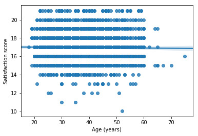
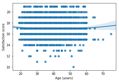
# fit second order polynomial # run the 2 scatterplots together to get both linear and second order fit lines scat1 = seaborn.regplot(x="q201", y="Satis", scatter=True, order=2, data=sub1) plt.xlabel('Age (years)') plt.ylabel('Satisfaction score')

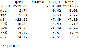
# center quantitative IVs for regression analysis sub1['q201_c'] = (data['q201'] - data['q201'].mean()) sub1['hoursweekavg_c'] = (data['hoursweekavg'] - data['hoursweekavg'].mean()) sub1['q203_c'] = (data['q203'] - data['q203'].mean()) sub1[["q201_c", "hoursweekavg_c", "q203_c"]].describe()

# linear regression analysis reg1 = smf.ols('Satis ~ q201_c', data=sub1).fit() print (reg1.summary())

# quadratic (polynomial) regression analysis

# run following line of code if you get PatsyError 'ImaginaryUnit' object is not callable

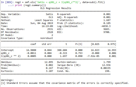
reg2 = smf.ols('Satis ~ q201_c + I(q201_c**2)', data=sub1).fit() print (reg2.summary())

################################################################ # EVALUATING MODEL FIT ################################################################

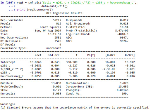
# adding education and hours worked per week on average into the model reg3 = smf.ols('Satis ~ q201_c + I(q201_c**2) + q203_c + hoursweekavg_c',               data=sub1).fit() print (reg3.summary())

#Q-Q plot for normality fig4=sm.qqplot(reg3.resid, line='r')

# simple plot of residuals stdres=pandas.DataFrame(reg3.resid_pearson) plt.plot(stdres, 'o', ls='None') l = plt.axhline(y=0, color='r') plt.ylabel('Standardized Residual') plt.xlabel('Observation Number')

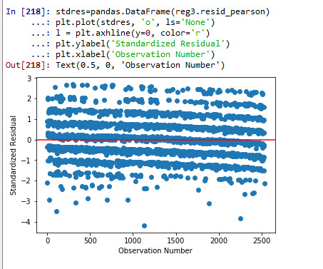
#explanation: we have some outliers outside + and - 2 std. of mean but not extreme outliers beyond + and -3 sd. of mean.

#explanation: fit of model was relatively poor, and we should included more explanatory variables

# additional regression diagnostic plots fig3 = plt.figure(figsize=(12,8)) fig3 = sm.graphics.plot_regress_exog(reg3,"hoursweekavg_c", fig=fig3)

# leverage plot fig3=sm.graphics.influence_plot(reg3, size=8) print(fig3)

#explanation: we don’t have any observations which have high residuals and high leverage

Interpretation

When examining the association between age and satisfaction score--- which the variable of interest, we found a non significant relationship (Beta=-0.0024, p=0.5). I further added a quadratic term of age into the model, the result of analysis showed the term was not statistically significant (Beta=0.0005, p=0.090). Further I included other explanatory variables into the model. Years of completed education was statistically significantly associated with each year increase in completed years of education associated with 0.08 points decrease in satisfaction score (Beta=-0.08, p<0.001). Final term included into the model was hours worked on average each week which was not statistically associated with satisfaction score (Beta=0.006, p=0.2).

A number of diagnostic test of residuals were performed for checking the fit of regression model. The Q-Q plot showed that the model is generally fitted well with exception for the lower and upper quartile of explanatory variable. Similarly, analyzing the standardized residuals of all observation, the analysis identified presence of some outliers outside of + and - 2 std. of mean but not any extreme outliers outside of + and -3 sd. of mean. The fit of model was relatively poor, which hints at including more explanatory variables to improve the fit of the model. Finally, the leverage plot confirmed the absence of observations with both high residuals and high leverage. 

Finally, our analysis suggests that the age is not strong predictor of work satisfaction among community health workers. Unlike age, the analysis revealed that education is a strong predictor of work satisfaction adjusting potential confounding variable such as age and hours worked per week.

[shivarajmishra]

DSW2. Regression modeling in practice (Python Programming)

#Project: Demographic profiling of community health workers in Nepal

#Dataset: fchv2014workingdata.csv, more info, link https://bit.ly/2T3fuV2

#loading the library first 

import numpy as numpyp import pandas as pandas import statsmodels.api import statsmodels.formula.api as smf

# bug fix for display formats to avoid run time errors

pandas.set_option('display.float_format', lambda x:'%.2f'%x)

#loading our dataset for this analysis

data = pandas.read_csv('fchv2014workingdata.csv', low_memory=False)

# convert variables to numeric format using convert_objects function

data['Satis'] = pandas.to_numeric(data['Satis'], errors='coerce') data['q201'] = pandas.to_numeric(data['q201'], errors='coerce')

#centering age around mean

data['q201'] = (data['q201'] - data['q201'].mean())

# BASIC LINEAR REGRESSION

#quantitative explanatory variable scat1 = seaborn.regplot(x="q201", y="Satis", scatter=True, data=data) plt.xlabel('Age') plt.ylabel('Satisfaction score') plt.title ('Scatterplot for the Association Between age and satisfaction score') print(scat1)

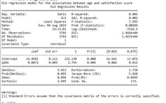
print ("OLS regression model for the association between age and satisfaction score") reg1 = smf.ols('Satis ~ q201', data=data).fit() print (reg1.summary())

#categorical explanatory variable 

def score_to_numeric2(x):    if x=='<25 yr':        return 1    if x=='40-54 yr':        return 3    if x=='25-39 yr':        return 2    if x=='55+ yr':        return 4 data['age'] = data['age'].apply(score_to_numeric2) data

scat1 = seaborn.regplot(x="age", y="Satis", scatter=True, data=data) plt.xlabel('Age') plt.ylabel('Satisfaction score') plt.title ('Scatterplot for the Association Between age groups (years) and satisfaction score') print(scat1)

print ("OLS regression model for the association between age groups (years) and satisfaction score") reg1 = smf.ols('Satis ~ age', data=data).fit() print (reg1.summary())

Interpretation

The results of the linear regression analysis indicated that age (years) (Beta=0.007, p=0.006) was significantly and positively associated with satisfaction score (1). In this analysis age was centered around mean value.

Satisfaction=16.9+0.007*age----(1)

When the age was entered into the model as a categorical variable, the regression model was fitted as (B=0.7, p=0.07) (2),

Satisfaction=17+0.07*age---(2)

Overall, each year increase in age was associated with a small increase in overall satisfaction score when the model is fitted with age as a continuous variable (p=0.006), and marginally associated when the model is fitted with age as categorical variable (<25, 25-39, 40-54, 55+ yr) (p=0.07).

[shivarajmishra]

DSW1. Regression modeling in practice (Python Programming)

Project: Demographic profiling of community health workers in Nepal

Sample

The data for this study is taken from “Female community health volunteers national survey” conducted by John Snow Research Institute (JSI) in 2014. The study comprised ~4000 CHWs from 13 domains across 75 districts of Nepal. A systematic random sampling technique was used with ward as the smallest geographic unit. A sampling interval was used to select ‘kth’ ward until the required sample for size each of these 13 domains was reached. A total of 4313 respondents were included in the survey and the same number is analysed in this study. The full description of study and questionnaire used is found elsewhere (1).

Procedure

The unit of data collection were FCHVs. One or more FCHVs were selected from each ward--the smallest geographic unit in Nepal. A mobile data collection platform called Enketo was set up for data collection, linking it with another data platform Survey CTO for storing the collected data. 

Measures 

The work satisfaction of FCHV’s was recorded as a set of 21 questions inquiring about factors influencing CHW’s motivation/satisfaction. CHWs were asked to rate each statement:  somewhat agree (+1); completely agree (+2); somewhat disagree (-1); or completely disagree (-2). Both ‘completely disagree and ‘somewhat disagree’ were recorded as ‘no’ and both ‘somewhat agree’ and ‘completely agree’ were coded as ‘no’. ‘Unsure/neutral’ responses were marked as missing. Based on this classification, we further created a variable called ‘satis’ by adding up a set of 21 variables, which was categorized into ‘Satisfied’ and ‘Unsatisfied’ based on median value of satisfaction score. Further, the distribution of this aggregate variable was checked based on quartile and constomized split.

In this analysis I am particularly interested in examining the association between demographic factors (eg. age, education) with satisfaction score.

The codebook including the variables, and specific questions asked in the survey is presented in Table 1 in the link below.

Table 1: Codebook showing the variables used and the specific questions asked in the survey

https://docs.google.com/spreadsheets/d/1RsMlXXropyEFMFTaA9N_XeYiu77InRXPjpmlpMLsuc8/edit?usp=sharing

References

1. Ministry of Health and Population. Female Community Health Volunteer National Survey Report 2014 Kathmandu: MOHP/JSI; 2014 [Available from: https://www.advancingpartners.org/sites/default/files/sites/default/files/resources/fchv_2014_national_survey_report_a4_final_508_0.pdf.

[shivarajmishra]

DSW4 Data Analysis Tools (Python): Statistical Interactions

Project: ‘Demographic profiling of community health workers in Nepal’.

#first setting up the library

import numpy import pandas import statsmodels.formula.api as smf import statsmodels.stats.multicomp as multi import seaborn import matplotlib.pyplot as plt

data = pandas.read_csv('fchv2014workingdata.csv', low_memory=False)

data = data[['Satis', 'q203', 'age']].dropna()

#Education q203

print ('education composition in the study sample') c1 = data['q203'].value_counts(sort=False) print (c1)

#converting Satisfaction score into four categories based on customized splits

data['edu3cat'] = pandas.cut(data.q203, [0, 5, 8, 13]) c2 = data['edu3cat'].value_counts(sort=False, dropna=True) print(c2)

#printing to see if it is dichotomized well

sub1=data[['q203', 'edu3cat']] a = sub1.head (n=1000) print(a)

print ('education composition in the study sample') c1 = sub1['edu3cat'].value_counts(sort=False) print (c1)

model1 = smf.ols(formula='Satis ~ C(edu3cat)', data=data).fit() print (model1.summary())

sub2 = data[['Satis', 'edu3cat']].dropna()

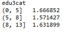
print ("means for Satisfaction Score by Age groups (years)") m1= sub2.groupby('edu3cat').mean() print (m1)

print ("standard deviation for Satisfaction Score by Age groups (years)") st1= sub2.groupby('edu3cat').std() print (st1)

# bivariate bar graph

seaborn.factorplot(x="edu3cat", y="Satis", data=sub2, kind="bar", ci=None) plt.xlabel('Education') plt.ylabel('Mean Satisfaction Score')

#now we will be examining the association between education and satisfaction score by third variable age

sub3=data[(data['age']=='<25 yr')] sub4=data[(data['age']=='25-39 yr')] sub5=data[(data['age']=='40-54 yr')] sub6=data[(data['age']=='55+ yr')]

#now we are running the ANOVA test for each level of third variable

#<25 yr print ('association between education and satisfaction score for those aged <25 yrs') model2 = smf.ols(formula='Satis ~ C(edu3cat)', data=sub3).fit() print (model2.summary())

print ("means for satisfaction score by education status for those aged <25 yrs") m3= sub3.groupby('edu3cat').mean() print (m3)

#25-39 yr print ('association between education and satisfaction score for those aged 25-39 yrs') model2 = smf.ols(formula='Satis ~ C(edu3cat)', data=sub4).fit() print (model2.summary())

print ("means for satisfaction score by education status for those aged 25-39 yrs") m3= sub4.groupby('edu3cat').mean() print (m3)

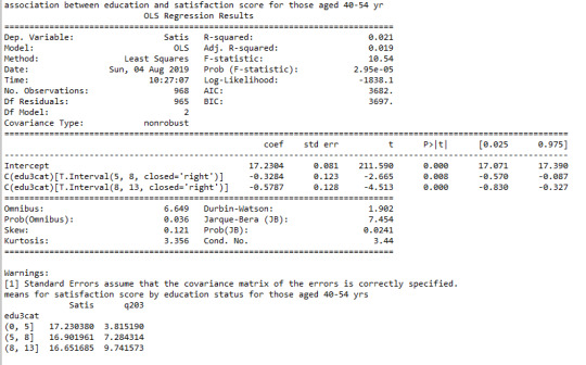
#40-54 yr print ('association between education and satisfaction score for those aged 40-54 yr') model2 = smf.ols(formula='Satis ~ C(edu3cat)', data=sub5).fit() print (model2.summary())

print ("means for satisfaction score by education status for those aged 40-54 yrs") m3= sub5.groupby('edu3cat').mean() print (m3)

#55+ yr print ('association between education and satisfaction score for those aged 55+ yrs') model2 = smf.ols(formula='Satis ~ C(edu3cat)', data=sub6).fit() print (model2.summary())

print ("means for satisfaction score by education status for those aged 55+yrs") m3= sub6.groupby('edu3cat').mean()

Interpretation

The mean satisfaction score among CHW’s with 0-5, 5-8 and 8-13 years of completed education was following: 17.2(sd.1.7), 17.0(sd.1.6), and 16.7(sd.1.6). When examining the association between completed years of education and satisfaction score by third moderator variable age, ANOVA revealed that the mean satisfaction score decreased as completed years of education increased (F=21, p<0.001) with only apparent relationship among those aged 25-39 yr (F=12, p<0.001), 40-54 yr (F=11, p<0.001) and 55+ yr (F=4, p=0.01) and no statistical relationship among aged <25 yr (F=0.6, p=0.6).

[shivarajmishra]

DSW3 Data Analysis Tools (Python)

Project: ‘Demographic profiling of community health workers in Nepal’.

#first setting up the library

import pandas import numpy import seaborn import scipy import matplotlib.pyplot as plt

data = pandas.read_csv('fchv2014workingdata.csv', low_memory=False)

#we are working with two variables 'satis' and 'q201' which both are continuous

#setting variables you will be working with to numeric data['q201'] = data['q201'].convert_objects(convert_numeric=True) data['Satis'] = data['Satis'].convert_objects(convert_numeric=True) data['hoursweekavg'] = data['hoursweekavg'].convert_objects(convert_numeric=True)

data['q201']=data['q201'].replace(' ', numpy.nan) data['Satis']=data['Satis'].replace(' ', numpy.nan) data['hoursweekavg']=data['hoursweekavg'].replace(' ', numpy.nan)

#Age (years) and satisfaction score  

scat1 = seaborn.regplot(x="q201", y="Satis", fit_reg=True, data=data) plt.xlabel('Age (years)') plt.ylabel('Satisfaction score') plt.title('Scatterplot for the Association Between Age and Satisfaction')

#Age (years) and hours on average per week

scat2 = seaborn.regplot(x="hoursweekavg", y="Satis", fit_reg=True, data=data) plt.xlabel('Hours worked on average') plt.ylabel('Satisfaction score') plt.title('Scatterplot for the Association Between Hours Worked on Average Per Week and Satisfaction Score')

#dropping the missing values from dataset

sub1 = data[['Satis', 'q201', 'hoursweekavg']].dropna()

sub1=sub1[['Satis', 'q201', 'hoursweekavg']] a = sub1.head (n=100) print(a)

# Pearson statistics and p-value 

print ('association between Between Age and Satisfaction') print (scipy.stats.pearsonr(sub1['q201'], sub1['Satis']))

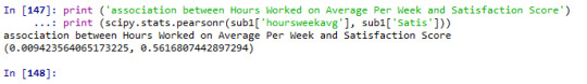
print ('association between Hours Worked on Average Per Week and Satisfaction Score') print (scipy.stats.pearsonr(sub1['hoursweekavg'], sub1['Satis']))

Interpretation:

We examined the Pearson correlation coefficient between two set of variables, 1) age (years) and satisfaction score, 2) hours worked per week on average and satisfaction score. 

First, the association between  age (years) and satisfaction score is statistically significant, r=0.044, p=0.005.Second, the association between  hours worked per week on average and satisfaction score however is not statistically significant, r=0.009, p=0.56.

[shivarajmishra]

DSW2 Data Analysis Tools (Python)

Project: ‘Demographic profiling of community health workers in Nepal’.

#first setting up the library

#load required library import pandas import numpy import statsmodels.formula.api as smf import statsmodels.stats.multicomp as multi import scipy.stats import seaborn import matplotlib.pyplot as plt

data=pandas.read_csv('fchv2014workingdata.csv', low_memory = False)

#converting Satisfaction score into two level satisfactor score based on median value of 17

def Satis_2cat (row):   if row['Satis'] >= 17 :      return 1   elif row['Satis'] < 17 :      return 0

data['Satis_2cat'] = data.apply (lambda row: Satis_2cat (row),axis=1)

c2= data.groupby('Satis_2cat').size()* 100 / len(data) print (c2) #printing to see if it is dichotomized well sub1=data[['Satis', 'Satis_2cat']] a = sub1.head (n=100) print(a)

#converting age into categorical variable

def score_to_numeric2(x):    if x=='<25 yr':        return 1    if x=='40-54 yr':        return 3    if x=='25-39 yr':        return 2    if x=='55+ yr':        return 4 data['age'] = data['age'].apply(score_to_numeric2) data

#SETTING MISSING DATA

data['age']=data['age'].replace(9, numpy.nan) data['Satis']=data['Satis'].replace(99, numpy.nan)

# contingency table of observed counts

ct1=pandas.crosstab(sub1['Satis_2cat'], data['age']) print (ct1)

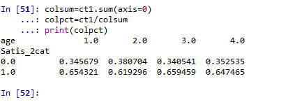
# column percentages

colsum=ct1.sum(axis=0) colpct=ct1/colsum print(colpct)

# chi-square

print ('chi-square value, p value, expected counts') cs1= scipy.stats.chi2_contingency(ct1) print (cs1)

# set variable types 

data["age"] = data["age"].astype('category') # new code for setting variables to numeric: sub1['Satis_2cat'] = pandas.to_numeric(sub1['Satis_2cat'], errors='coerce')

# loading the pandas library as well as program to run bar graph

import pandas as pd import seaborn as sns import matplotlib.pyplot as plt

# graph percent with satisfaction score >=17 within each age groups 

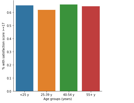
fake = pd.DataFrame({'age': ['<25 y', '25-39 y', '40-54 y','55+ y'], 'Satis_2cat':[0.654321, 0.619296, 0.659459, 0.647465]}) seaborn.factorplot(x="age", y="Satis_2cat", kind="bar", ci=None, data=fake) plt.xlabel('Age groups (years)') plt.ylabel('% with satisfaction score >=17')

Interpretations

When examining the association between CHW’s satisfaction score  (>=17, <17) and their age, a chi-square test of independence showed that those aged 25-39 y (62%), 40-54 y (66%), and 55+ (65%) have a similar satisfaction score >=17 compared to those aged 25 years (65%), X2=5.8, 3 df, p=0.12.

The df or degree of freedom here is the explanatory variable: age groups which has four levels (df 4-1=3).

As there was no association between these two variable, therefore no post-hoc test was performed.

[shivarajmishra]

DSW1 Data Analysis Tools (Python)

Project: ‘Demographic profiling of community health workers in Nepal’.

#first setting up the library 

#current libraries import pandas import numpy import statsmodels.formula.api as smf import statsmodels.stats.multicomp as multi

#saving the dataset from previous week data.to_csv('fchv2014workingdata.csv')

#loading the dataset and checking the number of records and variables data=pandas.read_csv('fchv2014workingdata.csv', low_memory = False) print(len(data)) print(len(data.columns))

#there are three variables that we are working with today

#satis #continuous variable #age #categorical satisfaction variable into 4 categories

#q203 #continuous variable 

#age

#frequency distribution for age (categorical) in the study sample# print ('age composition in the study sample') c1 = data['age'].value_counts(sort=False) print (c1)

print ('age composition in the study sample') c1 = data['Satis'].value_counts(sort=False) print (c1)

#looking at the data structure sub1=data[['Satis']] a = sub1.head (n=100) print(a)

#converting age into categorical variable def score_to_numeric2(x):    if x=='<25 yr':        return 1    if x=='40-54 yr':        return 2    if x=='25-39 yr':        return 3    if x=='55+ yr':        return 4 data['age'] = data['age'].apply(score_to_numeric2) data

#setting missing data data['age']=data['age'].replace(9, numpy.nan) data['Satis']=data['Satis'].replace(99, numpy.nan)

# standard deviation and other descriptive statistics for quantitative variables print ('age composition in the study sample') c1 = data['age'].value_counts(sort=False) print (c1)

#ANOVA test

# using ols function for calculating the F-statistic and associated p value

#age model1 = smf.ols(formula='Satis ~ C(age)', data=data) results1 = model1.fit() print (results1.summary())

sub1 = data[['Satis', 'age']].dropna()

# drop rows with missing values sub1.dropna(inplace=True)

# summarize the number of rows and columns in the dataset print(sub1.shape)

print ('means satisfaction score by age groups (years)') m1= sub1.groupby('age').mean() print (m1)

print ('standard deviations for satis by major age groups (years)') sd1 = sub1.groupby('age').std() print (sd1)

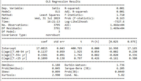
#post hoc using  Tukey's honest significance test tests for ANOVA comparing mean satisfaction score across age groups

sub1 = data[['Satis', 'age']].dropna() mc1 = multi.MultiComparison(sub1['Satis'], sub1['age']) res1 = mc1.tukeyhsd() print(res1.summary())

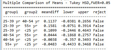
#Education q203 print ('education composition in the study sample') c1 = data['q203'].value_counts(sort=False) print (c1)

#converting Satisfaction score into two level satisfactor score based on median value of 17 data['edu3cat'] = pandas.cut(data.q203, [0, 5, 8, 13]) c2 = data['edu3cat'].value_counts(sort=False, dropna=True) print(c2)

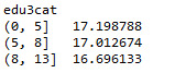
#printing to see if it is dichotomized well sub1=data[['q203', 'edu3cat']] a = sub1.head (n=1000) print(a)

print ('education composition in the study sample') c1 = data['edu3cat'].value_counts(sort=False) print (c1)

sub2 = data[['Satis', 'edu3cat']].dropna() # using ols function for calculating the F-statistic and associated p value model1 = smf.ols(formula='Satis ~ C(edu3cat)', data=data) results1 = model1.fit() print (results1.summary())

print ('means satisfaction score by age groups (years)') m1= sub2.groupby('edu3cat').mean() print (m1)

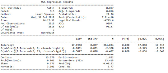
#Post-hoc test using Tukey's honest significance test

#post hoc tests for ANOVA comparing mean satisfaction score across education status variable sub2 = data[['Satis', 'edu3cat']].dropna() mc1 = multi.MultiComparison(sub2['Satis'], sub2['edu3cat']) res1 = mc1.tukeyhsd() print(res1.summary())

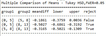
Interpretation

ANOVA comparing mean satisfaction score(satis) across age groups (age)

When examining,mean satisfaction score across age groups, ANOVA revealed that those aged <25 years, 25-39 years, 40-54 years, 55+ years had mean satisfaction score of 17.2(sd.±1.6) 17.1(±1.7),17.2(±1.6), and 17.2(±1.8) with F statistics of F(3,3791)=1.71, p=0.16. Considering mean scores, there was no apparent difference in satisfaction score across age groups.

On post-hoc analysis of mean satisfaction score across age groups found that no two age groups have statistically different mean satisfaction score. All the comparisons were statistically similar.

ANOVA comparing mean satisfaction score (satis) across educational status (edu3cat)

When examining,mean satisfaction score by education status, ANOVA revealed that those who completed 0-5 years of education (mean: 17.2 ± 1.7) have higher satisfaction score compared to 5-8 (mean: 17.0 ± 1.6) and 9-13 years of education (mean:16.7 ± 1.6), with F statistics : F(2,2516) = 21.26, p<0.001.

On post-hoc analysis of mean satisfaction score by educational status found that those with 0-5 years (meandiff=0.5 score) and 5-8 years (meandiff=0.31 score)   of education had statistically higher satisfaction score compared to 8-13 years of education. All the comparisons were statistically similar.

[shivarajmishra]

DSW4: Setting up a data science project (Python)

Project: Demographic profiling of community health workers in Nepal.

#start with loading the library

import seaborn import matplotlib.pyplot as plt 

print ('Distribution of satisfaction score')

desc1 = data['Satis'].describe() print (desc1)

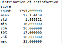
#the variable being considered is a numeric one. With mean of 17.15 and median of 17.

#univariate bar graph for categorical variables, first change the variables into categorical type

data["q701"] = data["q701"].astype('category')

data["q702"] = data["q702"].astype('category')

data["q703"] = data["q703"].astype('category')

data["q704"] = data["q704"].astype('category')

data["q705"] = data["q705"].astype('category')

data["q706"] = data["q706"].astype('category')

data["q707"] = data["q707"].astype('category')

data["q708"] = data["q708"].astype('category')

data["q709"] = data["q709"].astype('category')

data["q710"] = data["q710"].astype('category')

data["q711"] = data["q711"].astype('category')

data["q712"] = data["q712"].astype('category')

data["q713"] = data["q713"].astype('category')

data["q714"] = data["q714"].astype('category')

data[”q715"] = data["q715"].astype('category')

data["q716"] = data["q716"].astype('category')

data["q717"] = data["q717"].astype('category')

data["q718"] = data["q718"].astype('category')

data["q719"] = data["q719"].astype('category')

data["q720"] = data["q720"].astype('category')

data["q721"] = data["q721"].astype('category')

print ('describe individual satisfaction variable') desc2 = data['q701'].describe() print (desc2)

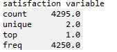
#this exactly reflects the variable being considered is changed into categorical varialbe from numeric.

#recording age variable

print ('age') c1 = data['q201'].value_counts(sort=False, dropna=False) print(c1)

data['Age1'] = pandas.cut(data.q106, [25, 39, 40, 54, 71]) c2 = data['Age1'].value_counts(sort=False, dropna=True) print(c2)

data['Satis'] = data['Satis'].convert_objects(convert_numeric=True) data['Age1'] = data['Age1'].convert_objects(convert_numeric=True)

#now we are interested in looking at whether age, education and residence affect satisfaction among community health workers

#bar graph for satisfaction score by age groups  

seaborn.factorplot(x='Age1', y='Satis', data=data, kind="bar", ci=None)

plt.xlabel('agegroups')

plt.ylabel('Satisfaction score by agegroups')

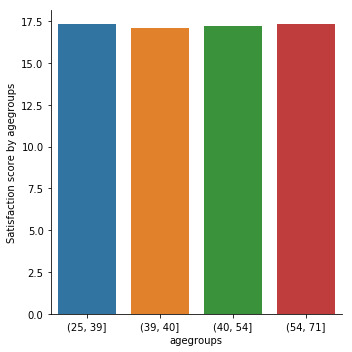
#bar graph for satisfaction score by caste  

plt.rc("figure", figsize=(45, 10))

seaborn.factorplot(x='caste', y='Satis', data=data, kind="bar", ci=None, size=4, aspect=2)

plt.xlabel('Caste')

plt.ylabel('Satisfaction score by caste')

#bar graph for satisfaction score by education  

seaborn.factorplot(x='education1', y='Satis', data=data, kind="bar", ci=None, size=4, aspect=2)

plt.xlabel('Education')

plt.ylabel('Satisfaction score by education')

#bar graph for satisfaction score by residence

seaborn.factorplot(x='residence', y='Satis', data=data, kind="bar", ci=None, size=4, aspect=2)

plt.xlabel('Residence')

plt.ylabel('Satisfaction score by residence')

#bar graph for satisfaction score by yrexperience  

seaborn.factorplot(x='yrexperience', y='Satis', data=data, kind="bar", ci=None, size=4, aspect=2)

plt.xlabel('years of experience as CHWs')

plt.ylabel('Satisfaction score by years of experience')

#converting Satisfaction score into two level satisfaction score based on median value of 17 as cut off

def Satis_2cat (row):

  if row['Satis'] >= 17 :

     return 1

  elif row['Satis'] < 17 :

     return 0

data['Satis_2cat'] = data.apply (lambda row: Satis_2cat (row),axis=1)

c2= data.groupby('Satis_2cat').size()* 100 / len(data) print (c2) #printing to see if it is dichotomized well sub1=data[['Satis', 'Satis_2cat']] a = sub1.head (n=100) print(a)

#bar chart with categorical satisfaction variable (yes, no)

print (p1)

seaborn.factorplot(x='Age1', y='Satis_2cat', data=data, kind="bar", ci=None)

plt.xlabel('agegroups')

plt.ylabel('Proportion satisfaction by agegroups')

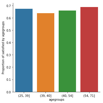
#basic scatterplot:  Q->Q: age and satisfaction score

scat1 = seaborn.regplot(x="q201", y="Satis", data=data)

plt.xlabel('age')

plt.ylabel('satisfaction score')

plt.title('Scatterplot for the Association Between age and satisfaction')

#basic scatterplot:  Q->Q: education and satisfaction score

scat1 = seaborn.regplot(x="q203", y="Satis",  data=data)

plt.xlabel('education')

plt.ylabel('satisfaction score')

plt.title('Scatterplot for the Association Between age and satisfaction')

Interpretation

I analyzed the distribution of satisfaction score by demographic variables: age, caste, education and residence, and years of experience. Except for residence there was no notable difference in satisfaction score by demographic variables. Rural community health workers had a marginally higher satisfaction score compared to their urban counterparts. I used the median as the cut off score to classify the satisfaction score into ‘Satisfied’ and ‘Unsatisfied’. There was a marginal increase in satisfaction score with aging. Using the Q-Q plot, we found a decreasing satisfaction score with increasing completed years of education. 

[shivarajmishra]

DSW3 Setting up a datascience project (Python)

Project: Demographic profiling of community health workers in Nepal. 

 The WEEK-3 assignments which includes recording and classification of variables into categories are illustrated in the python syntaxes below.

#coding missing data # frequencies of 21 variables 

#in the syntax below I am going to check the missing data on the following outcome variables which will be recorded later

print ('I am happy to be an CHW') c1 = data['q701'].value_counts(sort=False, dropna=False) print(c1) #2 missing data

print ('Five years from now I expect to sill be working as an CHW') c1 = data['q702'].value_counts(sort=False, dropna=False) print(c1) #2 missing data

print ('My community recognize and appreciate the services I provide') c1 = data['q703'].value_counts(sort=False, dropna=False) print(c1) #2 missing data

print ('Working as an CHW has contributed to receiving greater respect in my community') c1 = data['q704'].value_counts(sort=False, dropna=False) print(c1) #2 missing data

print ('My family supports my work as an CHW') c1 = data['q705'].value_counts(sort=False, dropna=False) print(c1) #2 missing data

print ('I receive enough support from my supervisor at the health facility') c1 = data['q706'].value_counts(sort=False, dropna=False) print(c1) #2 missing data

print ('Regular supplies of drugs and other supplies that I require') c1 = data['q707'].value_counts(sort=False, dropna=False) print(c1) #2 missing data

print ('I feel that I am treated fairly and respectfully by HWs at HFs') c1 = data['q708'].value_counts(sort=False, dropna=False) print(c1) #2 missing data

print ('Current provision of incentives is adequate for me') c1 = data['q709'].value_counts(sort=False, dropna=False) print(c1) #2 missing data

print ('My duties as an CHW interferes with other important responsibilities') c1 = data['q711'].value_counts(sort=False, dropna=False) print(c1) #2 missing data

print ('Filing in forms or registers related to my CHW duties is a burden to me') c1 = data['q712'].value_counts(sort=False, dropna=False) print(c1) #2 missing data

print ('At our local HF, we have a problem with certain HWs') c1 = data['q713'].value_counts(sort=False, dropna=False) print(c1) #2 missing data

print ('There have been problems at our HF with services not being provided properly') c1 = data['q714'].value_counts(sort=False, dropna=False) print(c1) #2 missing data

print ('As compared to the past, my work burden as an CHW has increased significantly') c1 = data['q715'].value_counts(sort=False, dropna=False) print(c1) #2 missing data

print ('Work as CHW provides opportunity to obtain new knowledge skills') c1 = data['q716'].value_counts(sort=False, dropna=False) print(c1) #2 missing data

print ('Work as CHW provides me respect and recognition from the community') c1 = data['q717'].value_counts(sort=False, dropna=False) print(c1) #2 missing data

print ('Work as CHW is a enjoyable, simulating and interesting activity') c1 = data['q718'].value_counts(sort=False, dropna=False) print(c1) #2 missing data

print ('Work as CHW contributes to family income') c1 = data['q719'].value_counts(sort=False, dropna=False) print(c1) #2 missing data

print ('Work as CHW helps people in the community can be healthier') c1 = data['q720'].value_counts(sort=False, dropna=False) print(c1) #2 missing data

print ('CHW work is a religious (dharma) duty to serve the community') c1 = data['q721'].value_counts(sort=False, dropna=False) print(c1) #2 missing data

#looking at the data structure

sub1=data[['q701','q702', 'q702', 'q703', 'q704', 'q705', 'q706', 'q707', 'q708',

          'q709', 'q710', 'q711', 'q712', 'q713', 'q714', 'q715', 'q716',

          'q717', 'q718', 'q719' , 'q720' , 'q721']]

a = sub1.head (n=100)

print(a)

#Note: for the above 21 variables, two records are missing consistently. And for other 20-40 records in each variable which has 'unsure' which will be flagged as ‘missing’.

def score_to_numeric(x):    if x=='somewhat agree':        return 1    if x=='totally agree':        return 1    if x=='totally disagree':        return 0    if x=='somewhat disagree':        return 0    if x=='unsure':        return 9  

data['q706_r'] = data['q706'].apply(score_to_numeric) data

# print 10 records to check a = data.head (n=10) print(a)

#printing 100 records to check sub1=data[['q701','q702', 'q706' , 'q706_r']] a = sub1.head (n=100) print(a)

#now applying this to all of the previous variable a701-q715

data['q701'] = data['q701'].apply(score_to_numeric)

data

data['q702'] = data['q702'].apply(score_to_numeric) data

data['q703'] = data['q703'].apply(score_to_numeric) data

data['q704'] = data['q704'].apply(score_to_numeric) data

data['q705'] = data['q705'].apply(score_to_numeric) data

data['q706'] = data['q706'].apply(score_to_numeric) data

data['q707'] = data['q707'].apply(score_to_numeric) data

data['q708'] = data['q708'].apply(score_to_numeric) data

data['q709'] = data['q709'].apply(score_to_numeric) data

data['q710'] = data['q710'].apply(score_to_numeric) data

data['q711'] = data['q711'].apply(score_to_numeric) data

data['q712'] = data['q712'].apply(score_to_numeric) data

data['q713'] = data['q713'].apply(score_to_numeric) data

data['q714'] = data['q714'].apply(score_to_numeric) data

data['q715'] = data['q715'].apply(score_to_numeric) data

#different set of definition for variable q716-q721

def score_to_numeric2(x):    if x=='somewhat important':        return 1    if x=='very important':        return 1    if x=='not important at all':        return 0    if x=='somewhat unimportant':        return 0    if x=='unsure':        return 9  

data['q716'] = data['q716'].apply(score_to_numeric2) data

data['q717'] = data['q717'].apply(score_to_numeric2) data

data['q718'] = data['q718'].apply(score_to_numeric2) data

data['q719'] = data['q719'].apply(score_to_numeric2) data

data['q720'] = data['q720'].apply(score_to_numeric2) data

data['q721'] = data['q721'].apply(score_to_numeric2) data

#checking one more time if the last variable q721 was recorded correctly

#printing 100 records to check sub1=data[['q701','q702', 'q702', 'q703', 'q704', 'q705', 'q706', 'q707', 'q708',           'q709', 'q710', 'q711', 'q712', 'q713', 'q714', 'q715', 'q716',           'q717', 'q718', 'q719' , 'q720' , 'q721']] a = sub1.head (n=100) print(a)

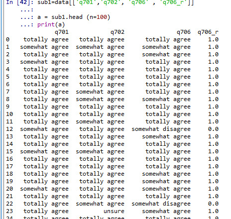
# recode 'unsure' as missing values  (NaN) data['q701']=data['q701'].replace(9, numpy.nan) data['q702']=data['q702'].replace(9, numpy.nan) data['q703']=data['q703'].replace(9, numpy.nan) data['q704']=data['q704'].replace(9, numpy.nan) data['q705']=data['q705'].replace(9, numpy.nan) data['q706']=data['q706'].replace(9, numpy.nan) data['q707']=data['q707'].replace(9, numpy.nan) data['q708']=data['q708'].replace(9, numpy.nan) data['q709']=data['q709'].replace(9, numpy.nan) data['q710']=data['q710'].replace(9, numpy.nan) data['q711']=data['q711'].replace(9, numpy.nan) data['q712']=data['q712'].replace(9, numpy.nan) data['q713']=data['q713'].replace(9, numpy.nan) data['q714']=data['q714'].replace(9, numpy.nan) data['q715']=data['q715'].replace(9, numpy.nan) data['q716']=data['q716'].replace(9, numpy.nan) data['q717']=data['q717'].replace(9, numpy.nan) data['q718']=data['q718'].replace(9, numpy.nan) data['q719']=data['q719'].replace(9, numpy.nan) data['q720']=data['q720'].replace(9, numpy.nan) data['q721']=data['q721'].replace(9, numpy.nan)

#creating secondary variables

#count of number of ethnicity categories endorsed, NUMETHNIC

data['Satis']=data['q701'] + data['q702'] + data['q703'] + data['q704'] + data['q705'] + data['q706'] + data['q707'] + data['q708'] + data['q709'] + data['q710'] + data['q711'] + data['q712'] + data['q713'] + data['q714'] + data['q715'] + data['q716'] + data['q717'] + data['q718'] + data['q719'] + data['q720'] + data['q721']

print('Satis')

#printing to see if they add up well

sub1=data[['q701','q702', 'q702', 'q703', 'q704', 'q705', 'q706', 'q707', 'q708',

          'q709', 'q710', 'q711', 'q712', 'q713', 'q714', 'q715', 'q716',

          'q717', 'q718', 'q719' , 'q720' , 'q721' , 'Satis']]

a = sub1.head (n=100)

print(a)

##running frequency distribution based on quartile and constumized splits

# quartile split (use qcut function & ask for 4 groups - gives you quartile split)

print ('Satisfaction - 4 categories - quartiles')

sub1['Satis']=pandas.qcut(sub1.Satis, 4, labels=["1=0%tile","2=25%tile","3=50%tile","4=75%tile"])

c1 = sub1['Satis'].value_counts(sort=False, dropna=True)

print(c1)

# categorize quantitative variable based on customized splits using cut function

# splits into 3 groups (11-14, 15-16, 17-18) - remember that Python starts counting from 0, not 1

data['Satis1'] = pandas.cut(data.Satis, [0, 14, 16, 18, 21])

c2 = data['Satis1'].value_counts(sort=False, dropna=True)

print(c2)

def score_to_numeric2(x):   if x=='somewhat important':       return 1   if x=='very important':       return 1   if x=='not important at all':       return 0   if x=='somewhat unimportant':       return 0   if x=='unsure':       return 9  

Interpretation

This analysis includes data from 4303 community health workers who participated in the survey. In this post, I coded the 21 variables related to perception and importance of work satisfaction expressed by community health workers into either ‘yes’ and ‘no’ category. Both ‘Totally agree and ‘Agree’ were recorded as ‘yes’ and both ‘Totally disagree’ and ‘Disagree’ was coded as ‘no’. Similarly, both ‘somewhat important’ and ‘very important’ was coded as ‘yes’ and both ‘not important at all’ and ‘somewhat unimportant’ was coded as ‘no’ in the analysis. Based on this classification, we further created a variable called ‘satis’ by adding up the variable from q701 to q721. Further, the distribution of this aggregate variable was checked based on quartile and constomized split.

This analysis  showed that the highest number of respondent were in the bottom quartile of satisfaction score (n=1360). Which equals to nearly 30% of participants. Similarly nearly a fifth of the CHWs were in highest quartile of satisfaction score (n=802).